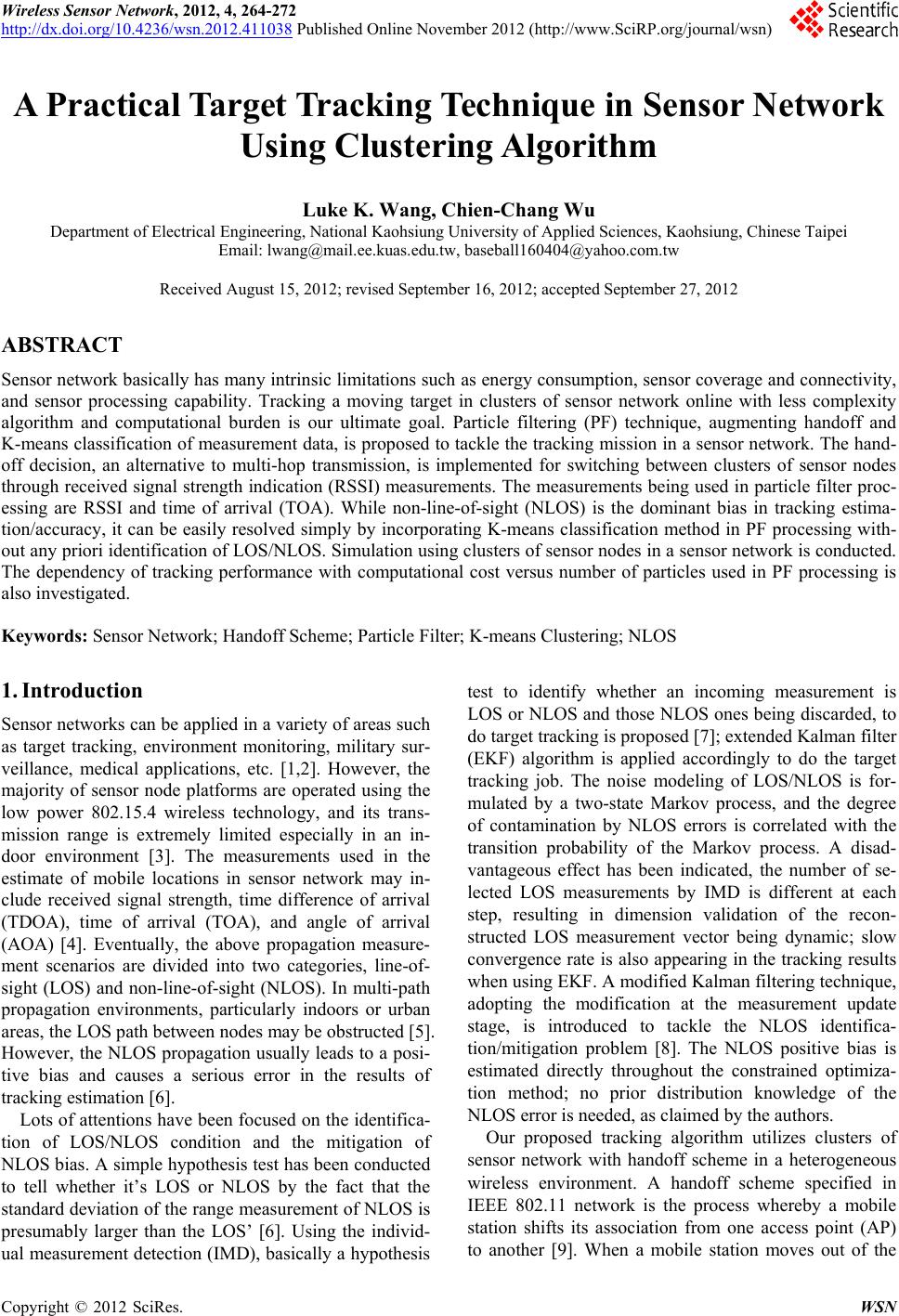Wireless Sensor Network, 2012, 4, 264-272
http://dx.doi.org/10.4236/wsn.2012.411038 Published Online November 2012 (http://www.SciRP.org/journal/wsn)
A Practical Target Tr acking Technique in Sensor Network
Using Clustering Algorithm
Luke K. Wang, Chien-Chang Wu
Department of Electrical Engineering, National Kaohsiung University of Applied Sciences, Kaohsiung, Chinese Taipei
Received August 15, 2012; revised September 16, 2012; accepted September 27, 2012
ABSTRACT
Sensor network basically has many intrinsic limitations such as energy consumption, sensor coverage and connectivity,
and sensor processing capability. Tracking a moving target in clusters of sensor network online with less complexity
algorithm and computational burden is our ultimate goal. Particle filtering (PF) technique, augmenting handoff and
K-means classification of measurement data, is proposed to tackle the tracking mission in a sensor network. The hand-
off decision, an alternative to multi-hop transmission, is implemented for switching between clusters of sensor nodes
through received signal strength indication (RSSI) measurements. The measurements being used in particle filter proc-
essing are RSSI and time of arrival (TOA). While non-line-of-sight (NLOS) is the dominant bias in tracking estima-
tion/accuracy, it can be easily resolved simply by incorporating K-means classification method in PF processing with-
out any priori identification of LOS/NLOS. Simulation using clusters of sensor nodes in a sensor network is conducted.
The dependency of tracking performance with computational cost versus number of particles used in PF processing is
also investigated.
Keywords: Sensor Network; Handoff Scheme; Particle Filter; K-means Clustering; NLOS
1. Introduction
Sensor networks can be applied in a variety of areas such
as target tracking, environment monitoring, military sur-
veillance, medical applications, etc. [1,2]. However, the
majority of sensor node platforms are operated using the
low power 802.15.4 wireless technology, and its trans-
mission range is extremely limited especially in an in-
door environment [3]. The measurements used in the
estimate of mobile locations in sensor network may in-
clude received signal strength, time difference of arrival
(TDOA), time of arrival (TOA), and angle of arrival
(AOA) [4]. Eventually, the above propagation measure-
ment scenarios are divided into two categories, line-of-
sight (LOS) and non-line-of-sight (NLOS). In multi-path
propagation environments, particularly indoors or urban
areas, the LOS path between nodes may be obstructed [5].
However, the NLOS propagation usually leads to a posi-
tive bias and causes a serious error in the results of
tracking estimation [6].
Lots of attentions have been focused on the identifica-
tion of LOS/NLOS condition and the mitigation of
NLOS bias. A simple hypothesis test has been conducted
to tell whether it’s LOS or NLOS by the fact that the
standard deviation of the range measurement of NLOS is
presumably larger than the LOS’ [6]. Using the individ-
ual measurement detection (IMD), basically a hypothesis
test to identify whether an incoming measurement is
LOS or NLOS and those NLOS ones being discarded, to
do target tracking is proposed [7]; extended Kalman filter
(EKF) algorithm is applied accordingly to do the target
tracking job. The noise modeling of LOS/NLOS is for-
mulated by a two-state Markov process, and the degree
of contamination by NLOS errors is correlated with the
transition probability of the Markov process. A disad-
vantageous effect has been indicated, the number of se-
lected LOS measurements by IMD is different at each
step, resulting in dimension validation of the recon-
structed LOS measurement vector being dynamic; slow
convergence rate is also appearing in the tracking results
when using EKF. A modified Kalman filtering technique,
adopting the modification at the measurement update
stage, is introduced to tackle the NLOS identifica-
tion/mitigation problem [8]. The NLOS positive bias is
estimated directly throughout the constrained optimiza-
tion method; no prior distribution knowledge of the
NLOS error is needed, as claimed by the authors.
Our proposed tracking algorithm utilizes clusters of
sensor network with handoff scheme in a heterogeneous
wireless environment. A handoff scheme specified in
IEEE 802.11 network is the process whereby a mobile
station shifts its association from one access point (AP)
to another [9]. When a mobile station moves out of the
C
opyright © 2012 SciRes. WSN

L. K. WANG, C.-C. WU 265
range of an AP and into another’s, the handoff occurs
during which there is an exchange of management
frames [10].
On the other hand, clustering analysis is the method of
unsupervised learning. It may include two parts, namely,
partitional clustering and hierarchical clustering. Parti-
tional clustering is a set of objects classified into K clus-
ters without hierarchical structure [11]. The clustering
method with PF can reduce the degradation of NLOS
propagation efficacy in tracking estimation results.
Meanwhile, handoff scheme is applied in the clusters of
sensor network. In clusters of sensor network, each clus-
ter has numbers of sensor nodes, including TOA and
RSSI sensors. Figure 1 shows the proposed architecture
that illustrates an event of target tracking in clusters of
sensor network.
The general approach to processing the LOS/NLOS
signals in cellular communication network is to deter-
mine whether it’s a LOS or NLOS condition. Even the
fuzzy inference scheme is introduced to tell whether it is
LOS or NLOS before any processing jobs can be done
[10]. It is combined with adaptive Kalman filter to estab-
lish mobile location estimator; undoubtedly, system and
computational complexities are increasing so tremen-
dously, hindering the potentials in real-time applications.
We present an architecture which utilizes clustering
analysis method with particle filter (PF) to track a mov-
ing target. Particle filter implements sequential Monte
Carlo simulation based on a set of particles to construct
prior density with associated weights for the approxima-
tion of posterior density.
The beneficial features of the proposed scenario are
listed as bellows,
 Intuitive but feasible for real-time applications due to
its low system and computational complexity attrib-
utes
Figure 1. The proposed architecture in clusters of sensor
network.
 No need to identify whether it is under LOS or NLOS
condition prior to any processing of the target loca-
tion estimation
 Only RSSI and TOA sensor measurements are re-
quired, practical and low-cost; fingerprinting scheme,
the build-up of a “radio map” database [6], and extra
hardware (sophisticated measurement devices) are not
employed, always leading to a low complexity, cost-
effective scenario.
 Both K-means clustering and hand-off schemes are
incorporated into the particle filter, minimizing the
system complexity to the most.
This analysis is set up as follows. The target’s motion
model and the associated measurement equation and
NLOS propagation are described in Section 2. Particle
filter is described in Section 3. Section 4 discusses the
proposed tracking algorithm which includes the handoff
scheme. The proposed tracking algorithm with clustering
method is derived in Section 5. The simulation and per-
formance analysis are presented in Section 6. Section 7
includes the conclusion.
2. Motion Models
We assume a mobile target’s movement is on a two-di-
mensional (2-D) plane. Besides, the measurement of
signal propagation with LOS/NLOS conditions may be
modeled as a two-state Markov process if the perform-
ance at transient stage is under investigation.
2.1. Target Model
The moving target’s state vector is defined as

T
1,kkkkk

x
xyy x, consisting of position and velocity
at a time instant k, where ()T stands for transpose opera-
tion of matrix. The target’s motion is modeled as
1,11,11,1  

kkk wA xx (1)
where
12
s
A
IA


1
01
s
s
T
A







and I2 is the 2  2 identity matrix;  is the Kronecker
product operator; A1 is the state transition matrix; s Tis
the sampling time; and is a zero mean white
Gaussian noise process with covariance matrix Q1, i.e.,
1, 1k
w


1, 11
~0,
k
wNQ
. The covariance matrix Q1 is
T
11,1,12kk s
QEwwqI Q




32
2
32
2
ss
s
ss
TT
QTT







where q1 is a scalar which determines the intensity of the

L. K. WANG, C.-C. WU
266
process noise and E[ ] is the expectation.
An alternative motion model may be described as be-
lo
k
(2)
Here
w,
2,2 2,12,1kk
Aw

xx

T
2,k kkkkkk

x
xxyyy  x;

,
kk

x
y represents
e position of the target;

,
kk
x
y

th and

,
kk

x
y
 
target
denote the
velocity and acceleration ongalong the x
and y directions, respectively. The transition matrix A2 is
given by
f the movi
2
22
12
01
00 1
ss
s
TT
AI T






Here . The covariance matrix Q2 is
av

2, 12
~0,
k
wNQ

transformingailable by a continuous-time stochastic
target model into an equivalent discrete-time model [12]:
2232
s
QqIQ
543
432
2
32
20 8 6
83
62
sss
ssss
ss s
TT
2QT TT
TT T





Here q2 is a scalar determining the intensity of the
pr
2.2. Measurement Model
s stationary, and its state
T
ocess noise.
Assume that our sensor node i
vector is
,,
jjj
ixiyi
s
ss


the ith sensor node in the jth cluster zone. The measure-
ment equation corresponding to TOA data can be formu-
lated as:
j
iTOA ki
cD s   x (3)
where c is the propagation speed of the transmitted signal;
xk is the state vector of the moving target; and i

is the
propagation time. The measurement equation wiNLOS
propagation error is shown as below,
th


N
LOS
kk k
zh xk . (4)
The measurement function h() models t
(5)
Here the random variable nlos has been mo
large scale of covariance value, usually hund
v
he TOA through
the ith sensor; vk is the measurement noise process inde-
pendent of w1,k−1, w2,k−1, and any other sensor noise
source; and the measurement noise is modeled by a zero
mean Gaussian white noise N (0,R). NLOSk is the NLOS
propagation error at the sampling instant k, modeled by a
two modes/states Markov process [13]. Therefore the
propagation error, NLOSk, is
0, i
f LOS present
NLOS , if NLOS present.
knlos


deled by a
red of me-
ters, of statistical distribution. An alternative measure-
ment model may be employed [12],


kkk kk
zh bnlosGnx (6)
where
0,if LOS presents
1,if NLOS presents
k
b 


0.5
NLOS
,if LOS presents
,if NLOS presents
m
k
m
G







bk is a binary sequence, modeled by a two-state, LOS and
NLOS, discrete-time Markov chain process and 
m is the
mportance sampling
ith some numbers of
typical standard deviation of LOS.
3. Particle Filter Pr oc essing
Particle filter is based on sequential i
(SIS) to estimate the system state w
particles with their associated weightings. Particle filter-
ing can be arranged to process the nonlinear and non-
Gaussian systems, and it has become an important alter-
native to the extended Kalman filter (EKF) [14]. There
are five processing stages in the implementation of PF,
i.e., initialization, particle propagation, weighting com-
putation, resampling, and estimation [14]. First of all,
particles are drawn from a proposal distribution at the
initialization step, where each particle possesses initial
weights. Then, the particle propagation is based on the
EKF to produce next state’s distribution. At the weight-
ing computation step, particle weights are set equal to the
ratio of probability distributions from the proposal dis-
tribution. The update equation of particle weighting can
be shown as [14]





1
iii
kk kk
ii
k
pzxpx x
ww 
1
1,
kii
kk k
qx x z


(7)
where the quantity ()ik denotes it is the ith
sampling time instant; q() is an importance density,
particle at kth
which can generate particles xi; and the likelihood func-
tion


i
kk
pz xis formulated by multivariate Gaussian
distribution,



1
11
ˆˆ exp T
kk
pzxz zRz z




2
2π
k kkk k
n
k
R
(8)
where


ˆ ˆk
zhx
utilize resam
with (^) standing for estimate value.
Here we pling strategy to eliminate part
w weighti
icles
with longs, and duplicates particles with larger
weighting. At the final step, it needs to calculate the cen-
ter of gravity from a group of samples. The PF algorithm

L. K. WANG, C.-C. WU 267
is summarized as below,
Particle Filter Algorithm
Step 1. Initialization
Draw initial samples


~
00
i
x
qx .
Set the weig 1/N where
icles us PF processing.
agation
on
hting of particles, 0
i
w, equal to
N is the number of parted in
Step 2. Particle Prop
Predict the next state of particles and update each par-
ticle by using EKF technique.
Step 3. Weighting Computati
Update the weightings with likelihood function


1
ii i
kk kk
wwpzx

.
Normalize the weighting for each particle
=1 .
kNi
k
iw

i
iw
k
w

Step 4. Resampli n g
N
j



where

=1
,N
ii
kk
i
xw





eff threshold
=1
=1
if
resampling ,
else
,
end
jj
kk
N
ii
kk
i
NN
xw
xw






 eff 1var i k
NN w
particles and var() stands
is the effective num-
ber of for taking the vari-
ance while Nthreshold is the prescribed threshold, usually
as 2/3 of the particle num
k
chosen ber.
Step 5. Estimation
Calculate the mean of particles with their associated
.
Nii
weightings, ˆk
1ik
x
wx

Tracking

4. Algorithm
The handoff scheme is applied to clusters of sensor net-
nal strength measurements
, and each cluster of RSSI
work, using the received sig
generated by the moving target
sensors provides the signal strength indications to switch
on/off the handoff.
For formulating the signal strength measurements, let
j
k

be the signal strength received by a moving target
from jth RSSI sensor at the kth sampling instant. The
re
the
ceived signal strengths can be modeled as a function of
distance plus a logarithmic of the shadowing compo-
nent [15], i.e.,
dbm
jjj
kkk
p   (9)
10 log
j
j
kj
pd  
k
(10)
whers the local signal power at
instan
ej
k
pi
t;
the kth sampling

is the path loss index; 
j is a co
mined by transmitted power, waveleng
t
nstant deter-
th, and antenna
gain ofhe jth RSSI sensor;
j
k
d is the distance between
the moving target and the jth RSSI sensor; andj
k

is the
logarithm of the shadow fading, modeled by a zero mean
Gaussian random process.
Handoff is triggered only if the current signal strength
drops below a user-defined threshold Δ, and any other
RSSI sensor’s strength is strr than that oft
on
c
onge
if
kr
the curren
e. Here 1
k
E is defined as the event with handoff being
triggered, and 0
k
E is the non-handoff situation [15,16],
that is,
1
0
if
krc
E
E



 




 (11)
where c

to
is the receive strength at mng tar-
get due current RSSI sennd
d signal
sor a
ovi
r

is the received
poweoving target ownio ance R sen-
r t
r at mng t refereSSI
sor othehan the current one. The conditional cost func-
tion is therefore defined

11, if
0, if
c
rk
CE




 (12)
c 
Handoff will be activated starting from tt
RSSI sensor to the candidate , when t
he curren
onehe cost function


1
rk
CE  is equal to 1 [15]oth Equations) and
(1
The can
. If b (11
2) are not satisfied, it means that there is no handoff
needed.
didate cluster of sensor network is chosen by
handoff decision, and measurements can be expressed
as
j
kk
zz

. Here the measurements follow Eqn (4),
a
uatio
n
e to be
d the given TOA measurement would be used in parti-
cle filter processing. Through PF processing, likelihoods
hav changed accordingly with handoff decision for
each particle,




j
i
kk kk
pz xpz x.
5. Tracking with K-Means Algorithm
The use of K-means method is to cluster theasure-
ing
2.
-
ith nui-
ial cents, are
e m
ack
ure
meric. In
roid
ment residual to be used in PF. The flowchart of tr
algorithm with clustering method is shown in Fig
5.1. K-means Clustering Method
K-means clustering is an unsupervised learning, compu
tationally efficient for large datasets w
tially, K samples, serving as the init
chosen at random from the whole sample space to ap-
proximate the centroids of initial clusters. The cluster
centroid is typically the mean of the data in the cluster.
Let


12
,,,
L
y
yyy be the dataset; ml is the cen-
troid of cluster Cl with Nl data points. The calculation of
the centroid of clusters is described as below,
1 ,1,2,, .
lll
mlk
NC


y
y (13)
where k is the number of clusters. First, initialize the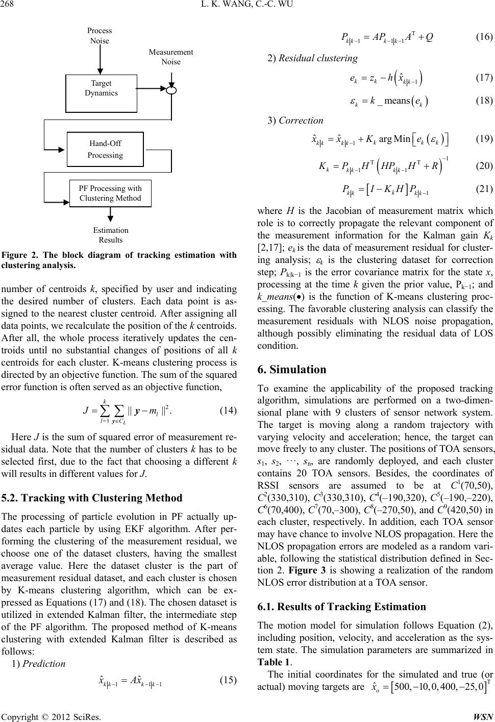

L. K. WANG, C.-C. WU
268
Target
Dynamics
Process
Noise
Hand-Off
Processing
PF Processing with
Clustering Method
Estimation
Results
Measurement
Noise
Figure 2. The block diagram of tracking estimation with
clustering analysis.
number of centroids k, specified by user andndicating
st cluster centroid. After assigning all
ata points, we recalculate the position of the k centroids.
e-
sidual data. Note that the number of clusters k has to be
selected first, due to the fact that choosi
will results in different values for J.
lgorithm. After per-
esidual, we
he smallest
i
the desired number of clusters. Each data point is as-
signed to the neare
d
After all, the whole process iteratively updates the cen-
troids until no substantial changes of positions of all k
centroids for each cluster. K-means clustering process is
directed by an objective function. The sum of the squared
error function is often served as an objective function,
2
=1
|||| .
L
k
l
lC
Jm



y
y (14)
Here J is the sum of squared error of measurement r
ng a different k
5.2. Tracking with Clustering Method
The processing of particle evolution in PF actually up-
dates each particle by using EKF a
forming the clustering of the measurement r
choose one of the dataset clusters, having t
average value. Here the dataset cluster is the part of
measurement residual dataset, and each cluster is chosen
by K-means clustering algorithm, which can be ex-
pressed as Equations (17) and (18). The chosen dataset is
utilized in extended Kalman filter, the intermediate step
of the PF algorithm. The proposed method of K-means
clustering with extended Kalman filter is described as
follows:
1) Prediction
111
ˆˆ
kkk k
xAx

 (15)
T
111kkk k
PAPAQ


 (16)
2) Residual clustering

(17)
1
ˆ
kk kk
ezhx


e

_ means
kk
k   (18)
3) Correction

kk 1
ˆˆ arg Min
k kk kk
xx Ke


 

(19)

1
TT
11
kkk kk
PHHPH

R

(20)
K


1
k
kk kk
PIKHP


where H is the Jacobian of measurement matrix which
role is to correctly propagate the relevant com
the measurement information for the Kalman gain K
[2,17]; ek is the data of measurement resi
ulations are performed on a two-dimen-
sional plane with 9 clusters of sensor network system.
ving along a random trajectory with
n as the sys-
tem state. The simulation parameters are summarized in
(21)
ponent of
k
dual for cluster-
ing analysis; 
k is the clustering dataset for correction
step; Pk|k−1 is the error covariance matrix for the state x,
processing at the time k given the prior value, Pk−1; and
k_means() is the function of K-means clustering proc-
essing. The favorable clustering analysis can classify the
measurement residuals with NLOS noise propagation,
although possibly eliminating the residual data of LOS
condition.
6. Simulation
To examine the applicability of the proposed tracking
algorithm, sim
The target is mo
varying velocity and acceleration; hence, the target can
move freely to any cluster. The positions of TOA sensors,
s1, s2, ···, sn, are randomly deployed, and each cluster
contains 20 TOA sensors. Besides, the coordinates of
RSSI sensors are assumed to be at C1(70,50),
C2(330,310), C3(330,310), C4(–190,320), C5(–190,–220),
C6(70,400), C7(70,–300), C8(–270,50), and C9(420,50) in
each cluster, respectively. In addition, each TOA sensor
may have chance to involve NLOS propagation. Here the
NLOS propagation errors are modeled as a random vari-
able, following the statistical distribution defined in Sec-
tion 2. Figure 3 is showing a realization of the random
NLOS error distribution at a TOA sensor.
6.1. Results of Tracking Estimation
The motion model for simulation follows Equation (2),
including position, velocity, and acceleratio
Table 1.
The initial coordinates for the simulated and true (or
actual) moving targets are

T
ˆ500,10,0, 400,25, 0
o
x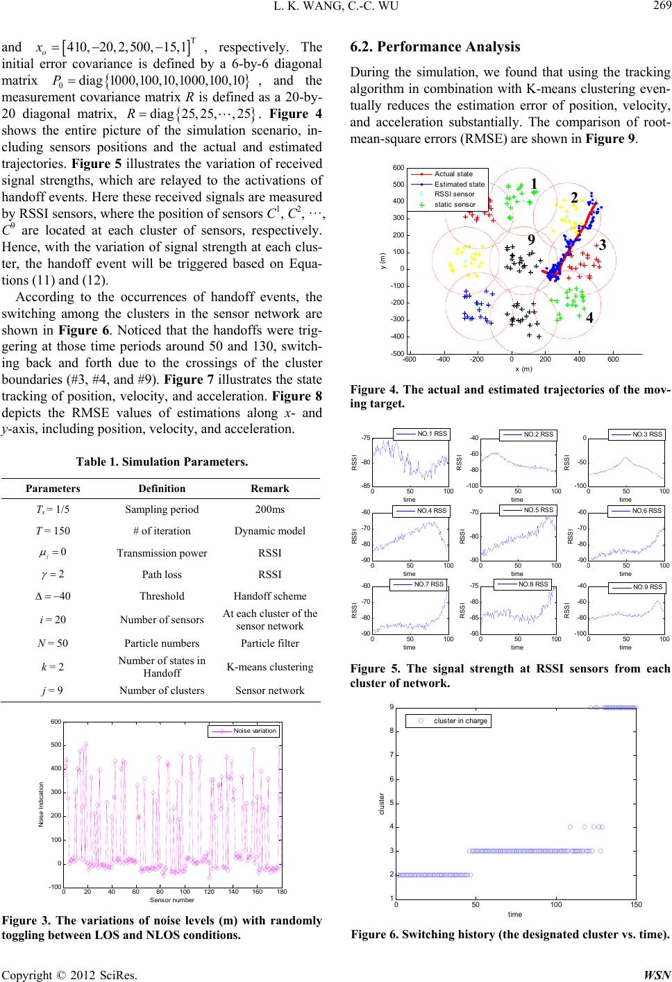

L. K. WANG, C.-C. WU 269
and

T
410,20,2,500, 15,1
o
x , respectively. The
initial error covariance is defined by a 6-by-6 diagonal
matrix

,100,10
0diag 1000,100,10,1000P
easurem
, and the
ment covariance matrix R is defined as a 20-by-
20 diagonal matrix,


5,, 25
riation
gnals ar
sings of
diag25, 2
s the entire picture of the sim
ies. Figure 5 illustrates the va
hese received si
due to the cros
R
showulation scenario, in-
cluding sensors positions and the actual and estimated
trajector of received
signal strengths, which are relayed to the activations of
handoff events. Here te measured
by RSSI sensors, where the position of sensors C1, C2, ···,
C9 are located at each cluster of sensors, respectively.
Hence, with the variation of signal strength at each clus-
ter, the handoff event will be triggered based on Equa-
tions (11) and (12).
According to the occurrences of handoff events, the
switching among the clusters in the sensor network are
shown in Figure 6. Noticed that the handoffs were trig-
gering at those time periods around 50 and 130, switch-
ing back and forth
. Figure 4
the cluster
boundaries (#3, #4, and #9). Figure 7 illustrates the state
tracking of position, velocity, and acceleration. Figure 8
depicts the RMSE values of estimations along x- and
y-axis, including position, velocity, and acceleration.
Table 1. Simulation Parameters.
Parameters Definition Remark
Ts = 1/5 Sampling period 200ms
T = 150 # of iteration
0
j
 
Dynamic model
RSSI Transmission power
2

 Path loss RSSI
40 Threshold Hand
At
sensor
Part
K-me
off scheme
e
k
ter
ans clustering
i = 20 Nurs
N = 50
k = 2 Nums in
j = 9 Number of clusters
mber of sensoeach cluster of th
networ
icle filParticle numbers
ber of state
Handoff
Sensor network
020 40 60 80100 120 140 160180
-100
0
100
200
300
400
500
600
Sensor num ber
Noise Indication
Noise variation
Figure 3. The variations of noise levels (m) with randomly
toggling between LOS and NLOS conditions.
6.2. Performance Analysis
During the simulation, we found that using the tracking
algorithm in combination with K-means clustering even-
tually reduces the estimation error of position, velocity,
and acceleration substantially. The comparison of root-
mean-square errors (RMSE) are shown in Figure 9.
600
-600 -400 -200 0200400 600
-500
-400
-300
-200
-100
0
100
200
300
400
500
x (m)
Actual state
Estimated state
RSSI sensor
static sensor
y (m)
2
1
igure 4. The actual and estimated trajectories of the mov-
ing target.
3
9
4
F
050 100
-85
-80
-75
time
RSSI
NO.1 RSS
050 100
-100
-80
-60
-40
time
RSSI
NO.2 RSS
050 100
-100
-50
0
time
RSSI
NO.3 RSS
050 100
-90
-80
-70
-60
time
RSSI
NO.4 RSS
050 100
-90
-80
-70
time
RSSI
NO.5 RSS
050 100
-90
-80
-70
-60
time
RSSI
NO.6 RSS
050 100
-90
-80
-70
-60
time
RSSI
NO.7 RSS
050 100
-90
-85
-80
-75
time
NO.8 RSS
RSSI
050 100
-100
-80
-60
-40
time
NO RS S
RSSI
.9
Figure 5. The signal strength at RSSI sensors from each
cluster of ne twork.
050100 150
1
9
2
3
4
5
6
7
c lust er in c harge
8
time
cluster
witching history (the designated cluster vs. time). Figure 6. S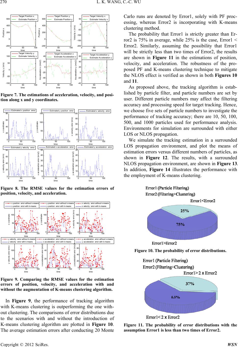

L. K. WANG, C.-C. WU
270
050 100
-200
0
200
400
600
time
Posit i on x
Target Position x
Estimate Position x
050 100
-200
0
200
400
600
time
Posit i on y
Target Position y
Estimate Position y
050 100
-200
-150
-100
-50
0
50
time
Velocity x (m/s)
Target Velocity x
Estimate Velocity x
050 100
-100
-50
0
50
100
time
Velocity y (m/s)
Target Velocity y
Estimate Velocity y
050 100
-60
-40
-20
0
20
40
time
Acc el erat i on x (m / s2)
Target Accelerat i on x
Estimate Acceleration x
050 100
-40
-20
0
20
40
60
time
Acc el erat i on y (m / s2)
Target Acc e leration y
Estimate Acceleration y
tion along x and y coordinates.
Figure 7. The estimations of acceleration, velocity, and posi-
050 100
0
20
40
60
80
time
x coordinat e
Es tim at ed x pos it i on error
050 100
0
50
100
150
time
y coordinat e
Esti m ated y posit i on error
050 100
0
20
40
60
80
100
time
x velocity error (m/s)
Estimated x velocity error
050 100
0
20
40
60
80
time
y velocity error (m/s)
Estimated y velocity error
050 100
0
10
20
30
40
50
time
x
ac cel era tion e rror (m/ s2)
Esti m ated x accelerati on error
050 100
0
10
20
30
40
50
time
y
ac cel era tion e rror (m/ s2)
Esti m ated y accelerati on error
F
position, velo
igure 8. The RMSE values for the estimation errors of
city, and acceleration.
050 100
0
50
100
150
time
x coordinat e
x posi ti on err or without k - me ans
x posi ti on err or with k-means
050 100
0
50
100
150
time
y coordinat e
y posi ti on err or without k - m eans
y posi ti on err or with k-means
050 100
0
50
100
150
time
x velocity error (m/s)
x velocity error wi thout k- m eans
x velocity error with k-means
050 100
0
50
100
150
time
y velocity error (m/s)
y velocity error without k-means
y velocity error with k-means
050 100
0
20
40
60
time
x acc eleration error (m/ s2)
x accele ration error without k-means
x acceleration error with k-means
050 100
0
20
40
60
80
time
y acc eleration error (m/ s2)
y accelera tion er ror wi thout k- m ean s
y accelera tion er ror wi th k - m eans
Figure 9. Comparing the RMSE values for the estimation
rrors of position, velocity, and acceleration with and
without the augmentation of K-means clustering algorithm.
In Figure 9, the performance of tracking algorithm
with K-means clustering is outperforming the one with-
out clustering. The comparisons of error distributions due
to the scenarios with and without the introduction of
K-means clustering algorithm are plotted in Figure 10.
The average estimation errors after conducting 20 Monte
Carlo runs are denoted by Error1, solely with PF proc-
essing, whereas Error2 is incorporating with K-means
clustering method.
The probability that Error1 is strictly greater than Er-
ror2 is 75% in average, while 25% is the case, Error1 <
Error2. Similarly, assuming the possibility that Error1
will be strictly less than two times of Error2, the results
are shown in Figure 11 in the estimations of position,
velocity, and acceleration. The robustness of the pro-
posed PF and K-means clustering technique to mitigate
the NLOS effect is verified as shown in both Figures 10
and 11.
As proposed above, the tracking algorithm is estab
e
-
lished by particle filter, and particle numbers are set by
user. Different particle numbers may affect the filtering
ccuracy and processing speed for target tracking. Hence, a
we choose five sets of particle numbers to investigate the
performance of tracking accuracy; there are 10, 50, 100,
500, and 1000 particles used for performance analysis.
Environments for simulation are surrounded with either
LOS or NLOS propagation.
We simulate the tracking estimation in a surrounded
LOS propagation environment, and plot the means of
estimation errors versus different numbers of particles, as
shown in Figure 12. The results, with a surrounded
NLOS propagation environment, are shown in Figure 13.
In addition, Figure 14 illustrates the performance with
the employment of K-means clustering.
Figure 10. The probability of error distributions.
Figure 11. The probability of error distributions with the
assumption Error1 is less than two times of Error2.

L. K. WANG, C.-C. WU 271
Figure 12. The results, estimation errors versus numbers of
particles, using solely par ticle filtering in a surrounded LOS
propagation environment.
Figure 13. The results, estimation errors versus numbers of
particles, using solely particle filtering in a surrounded
NLOS propagation environment.
Figure 14. The results, estimation errors versus numbers of
particles, using particle filtering with K-means clustering in
a surrounded NLOS propagation environment.
As the simulation results shown from Figure 12 to
Figure 14, each figure is simulated with 1000 time in-
stants, and we compute its associated estimation errors,
position, velocity, and acceleration.
As position, velocity, and acceleration are estimated,
not too much benefit can we expect in a LOS propaga-
tion environment when we vary the number of particles
in PF processing. The number of particles we choose is
50, being attractive in real-time tracking applications.
The estimation errors gradually reduce with the increase-
ing of particle numbers. On the contrary, situated in a
NLOS environment, substantial improvement of estima-
tion errors are illustrated in Figure 14 with K-means
clustering scenario; eventually, the trade-off among the
increment of particle numbers, estimation errors, and
e particle filter process-
g job.
7. Conclusions
Sophisticated and high system/computational complexity
algorithms are always proposed to mitigate the NLOS
effect and estimate the mobile/target location. In this
article, we propose a simple and feasible generic tracking
algorithm to track the moving target in clusters of sensor
network. The proposed tracking algorithm is the tech-
nique that adds handoff decision to the ordinary tracking
algorithm, based on TOA and RSSI measurements; the
handoff decision is implemented on clusters of sensor
network.
Besides, K-means clustering is utilized, and it com-
bines with particle filter to reduce the NLOS propagation
effect. Finally, the proposed algorithm can accom
[1] P. M. Djuric, M. Vemula and M. F. Bugallo, “Tracking
computational load is accomplished via the use of mod-
erate number of particle, i.e., 50, and the augmentation of
K-means clustering scheme in th
in
plish
higher accuracy in tracking estimation for sure.
Simulations illustrate that the estimation results of
tracking trajectory is well predicted, even around the
NLOS propagation environment. This analysis applies to
any motion modes, even with varying acceleration.
Moreover, we also compare the results of tracking algo-
rithm with and without K-means clustering in statistics.
Through the performance analysis, it demonstrates that
the proposed tracking algorithm may find potentials in
real-time tracking/localization applications as the particle
numbers used are reducing to as low as 50.
8. Acknowledgements
This work was partially supported by the National Sci-
ence Council of Taiwan, Republic of China under con-
tract NSC 99-2221-E-151-022.
REFERENCES

L. K. WANG, C.-C. WU
272
s,” IEEE International Conference on Acoustics
Signal Processing, 18-23 March 2005, pp.
.1109/ICASSP.2005.1416119
with Particle Filtering in Tertiary Wireless Sensor Net-
work
Speech and
ing Linear Programming in Ultrawideband Location-
Aware Networks,” IEEE Transactions on Vehicular
Technology, Vol. 56, No. 5, 2007, pp. 3182-3198.
doi:10.1109/TVT.2007.900397
[10] J. F. Liao and B. S. Chen, “Adaptive Mobile Loca
,
757-760. doi:10
ajah and S. Halgamuge, “Mobile Sensor [2] S. Maheswarartion
khool and S. Cherkaoui, “Handoff in IEEE
g Interacting Mul-
ansactions on Wireless
Management for Target Tracking,” 2nd International
Symposium on Wireless Pervasive Computing, San Juan,
5-7 February 2007, pp. 506-510.
doi:10.1109/ISWPC.2007. 342656
[3] J. Wu, H. Xiong, J. Chen and W. Zhou, “A Generaliza-
tion of Proximity Functions for K-means,” 7th IEEE In-
ternational Conference on Data Mining, Omaha, 28-31
October 2007, pp. 361-370.doi:10.1109/ICDM.2007.59
[4] J. F. Liao and B. S. Chen, “Robust Mobile Location Es-
timator with NLOS Mitigation Using Interacting Multiple
Estimator with NLOS Mitigation Using Fuzzy Inference
Scheme,” 8th International Symposium on Communica-
tions, Kaohsiung, Taiwan, 2005.
[11] B. S. Gu
802.11p-Based Vehicular Networks,” IFIP International
Conference on Wireless and Optical Communications
Networks, Cairo, 28-30 April 2009, pp. 1-5.
[12] J. F. Liao and B. S. Chen, “Robust Mobile Location Es-
timator with NLOS Mitigation Usin
tipke Model Algorithm,” IEEE Tr
Model Algorithm,” IEEE Transactions on Wireless Com-
munications, Vol. 5, No. 11, 2006, pp. 3002-3006.
doi:10.1109/TWC.2006.04747
[5] S. S. Moghaddam, V. T. Vakilim and A. Falahati, “New
Handoff Initiation Algorithm (Optimum Combin
Communications, Vol. 5, No. 11, 2006, pp. 3002-3006.
doi:10.1109/TWC.2006.04747
[13] C. C. Tseng, K. H. Chi, M. D. Hsieh and H. H. Chang
“Location-Based Fast H
,
andoff for 802.11 Networks,”
IEEE Communications Letters, Vol. 9, No. 4, 2005, pp.
304-306. doi:10.1109/LCOMM.2005.04010
[14] S. Arulampalam, S. Maskell, N. Gordon and T. Clapp, “A
Tutorial on Particle Filters for Online Nonlinear
Gaussian Bayesian Tracking,” IEEE Transactions on
ation of
Hysteresis & Threshold Based Methods),” 52nd IEEE
VTS-Fall VTC of Vehicular Technology Conference, Vol.
4, 2000, pp. 1567-1574. doi:10.1109/AMS.2009.11
[6] C.-D. Wann, “Kalman Filtering for NLOS Mitigation and
Target Tracking in Indoor Wireless Environment,” In: V.
Kordic, Ed., Kalman Filter, Intech Publication, 2010, pp.
16-33.
[7] L. Yi, S. G. Razul, Z. Lin and C.-M. See, “Target Track-
ing in Mixed LOS/NLOS Environments Based on Indi-
vidual TOA Measurement Detection,” IEEE Sensor Array
and Multichannel Signal Processing Work
/Non-
Signal Processing, Vol. 50, No. 2, 2002, pp. 174-188.
doi:10.1109/78.978374
[15] Z. Yang and X. Wang, “Joint Mobility Tracking and
Handoff in Cellular Networks via Sequential Monte Carlo
Filtering,” IEEE Transactions on Signal Processing, Vol.
51, No. 1, 2003, pp. 269-281.
doi:10.1109/TSP.2002.806580
[16] R. Prakash and V. Veeravalli, “Adaptive Ha
shop, Jerusa-
153-156.
06720
lem, 4-7 October 2010, pp.
doi:10.1109/SAM.2010.56 rd Handoff Algorithm,” IEEE Journal on Selected Areas in Commu-
nications, Vol. 18, 2000, pp. 2456-2464.
doi:10.1109/49. 895049
[17] G. Welch and G. Bishop, “An Introduction to the Kalman
Filter,” Technical Report, Univer
[8] W. Kei and L. Wu, “Mobile Location with NLOS Identi-
fication and Mitigation Based on Modified Kalman Fil-
tering,” Sensors, Vol. 11, No. 2, 2011, pp. 1641-1656.
doi:10.3390/s110201641
[9] S. Venkatesh and R. M. Buehrer, “NLOS Mitigation Us-
sity of North Carolina,
ty distribution
New Caledonia, 2002.
Nomenclature
Ai, i = 1, 2 State transition matrix
bk, k = 1, 2 Binary sequence (LOS or NLOS)
i
k
E, i = 0, 1 Handoff/non-Handoff event
NLOSk Measurement error at time instant k
p(|) Conditional probabili
q() Importance density
Xi,k, i = 1, 2 Target state vector at time instant k
i
k
W Weighting associated with ith particle at
time instant k