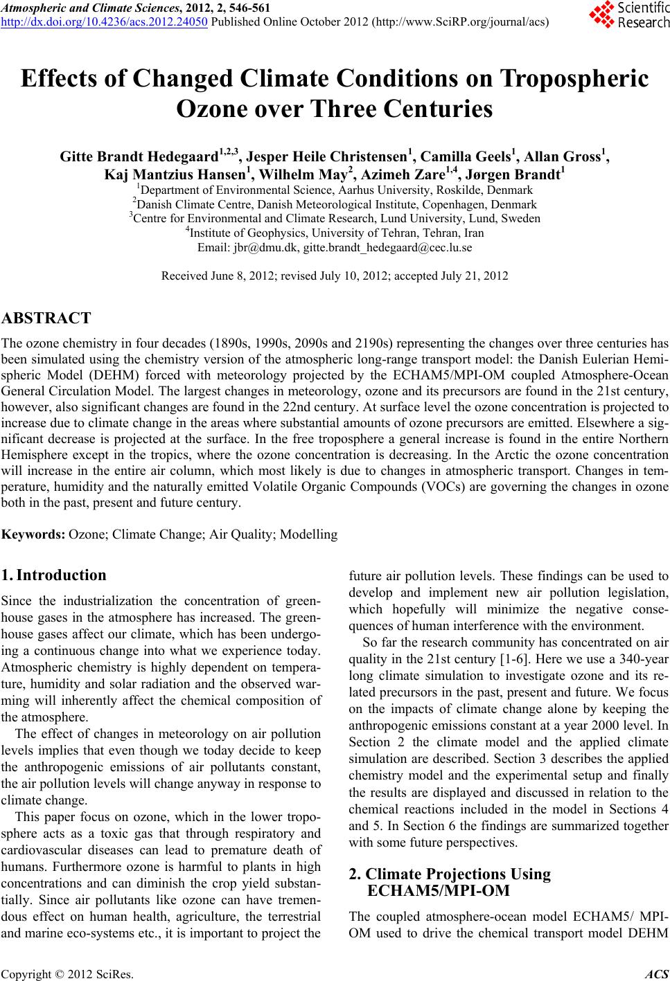
Atmospheric and Climate Sciences, 2012, 2, 546-561
http://dx.doi.org/10.4236/acs.2012.24050 Published Online October 2012 (http://www.SciRP.org/journal/acs)
Effects of Changed Climate Conditions on Tropospheric
Ozone over Three Centuries
Gitte Brandt Hedegaard1,2,3, Jesper Heile Christensen1, Camilla Geels1, Allan Gross1,
Kaj Mantzius Hansen1, Wilhelm May2, Azimeh Zare1,4, Jørgen Brandt1
1Department of Environmental Science, Aarhus University, Roskilde, Denmark
2Danish Climate Centre, Danish Meteorological Institute, Copenhagen, Denmark
3Centre for Environmental and Climate Research, Lund University, Lund, Sweden
4Institute of Geophysics, University of Tehran, Tehran, Iran
Received June 8, 2012; revised July 10, 2012; accepted July 21, 2012
ABSTRACT
The ozone chemistry in four decades (1890s, 1990s, 2090s and 2190s) representing the changes over three centuries has
been simulated using the chemistry version of the atmospheric long-range transport model: the Danish Eulerian Hemi-
spheric Model (DEHM) forced with meteorology projected by the ECHAM5/MPI-OM coupled Atmosphere-Ocean
General Circulation Model. The largest changes in meteorology, ozone and its precursors are found in the 21st century,
however, also significant changes are found in the 22nd century. At surface level the ozone concentration is projected to
increase due to climate change in the areas where substantial amounts of ozone precursors are emitted. Elsewhere a sig-
nificant decrease is projected at the surface. In the free troposphere a general increase is found in the entire Northern
Hemisphere except in the tropics, where the ozone concentration is decreasing. In the Arctic the ozone concentration
will increase in the entire air column, which most likely is due to changes in atmospheric transport. Changes in tem-
perature, humidity and the naturally emitted Volatile Organic Compounds (VOCs) are governing the changes in ozone
both in the past, present and future century.
Keywords: Ozone; Climate Change; Air Quality; Modelling
1. Introduction
Since the industrialization the concentration of green-
house gases in the atmosphere has increased. The green-
house gases affect our climate, which has been undergo-
ing a continuous change into what we experience today.
Atmospheric chemistry is highly dependent on tempera-
ture, humidity and solar radiation and the observed war-
ming will inherently affect the chemical composition of
the atmosphere.
The effect of changes in meteorology on air pollution
levels implies that even though we today decide to keep
the anthropogenic emissions of air pollutants constant,
the air pollution levels will change anyway in response to
climate change.
This paper focus on ozone, which in the lower tropo-
sphere acts as a toxic gas that through respiratory and
cardiovascular diseases can lead to premature death of
humans. Furthermore ozone is harmful to plants in high
concentrations and can diminish the crop yield substan-
tially. Since air pollutants like ozone can have tremen-
dous effect on human health, agriculture, the terrestrial
and marine eco-systems etc., it is important to project the
future air pollution levels. These findings can be used to
develop and implement new air pollution legislation,
which hopefully will minimize the negative conse-
quences of human interference with the environment.
So far the research community has concentrated on air
quality in the 21st century [1-6]. Here we use a 340-year
long climate simulation to investigate ozone and its re-
lated precursors in the past, present and future. We focus
on the impacts of climate change alone by keeping the
anthropogenic emissions constant at a year 2000 level. In
Section 2 the climate model and the applied climate
simulation are described. Section 3 describes the applied
chemistry model and the experimental setup and finally
the results are displayed and discussed in relation to the
chemical reactions included in the model in Sections 4
and 5. In Section 6 the findings are summarized together
with some future perspectives.
2. Climate Projections Using
ECHAM5/MPI-OM
The coupled atmosphere-ocean model ECHAM5/ MPI-
OM used to drive the chemical transport model DEHM
C
opyright © 2012 SciRes. ACS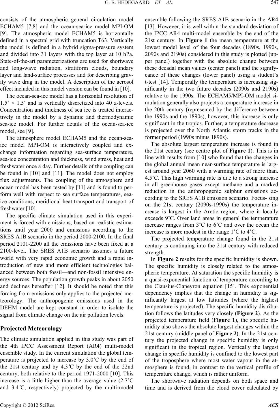

G. B. HEDEGAARD ET AL. 547
consists of the atmospheric general circulation model
ECHAM5 [7,8] and the ocean-sea-ice model MPI-OM
[9]. The atmospheric model ECHAM5 is horizontally
defined in a spectral grid with truncation T63. Vertically
the model is defined in a hybrid sigma-pressure system
and divided into 31 layers with the top layer at 10 hPa.
State-of-the-art parameterizations are used for shortwave
and long-wave radiation, stratiform clouds, boundary
layer and land-surface processes and for describing grav-
ity wave drag in the model. A description of the aerosol
effect included in this model version can be found in [10].
The ocean-sea-ice model has a horizontal resolution of
1.5˚ × 1.5˚ and is vertically discretized into 40 z-levels.
Concentration and thickness of sea ice is treated interac-
tively in the model by a dynamic and thermodynamic
sea-ice model. For further details of the ocean-sea-ice
model, see [9].
The atmosphere model ECHAM5 and the ocean-sea-
ice model MPI-OM is interactively coupled and ex-
change information regarding sea-surface temperature,
sea-ice concentration and thickness, wind stress, heat and
freshwater once a day. Further details of the coupling can
be found in [10] and [11]. The model does not employ
flux adjustments. The coupling of the atmosphere and
ocean model has been tested by [11] and is found to per-
form well with respect to sea surface temperatures, sea-
ice conditions, meridional heat transport and transport of
freshwater [10].
The specific climate simulation used in this experi-
ment is forced with emissions, based on realistic estima-
tions until year 2000 and emissions according to the
SRES A1B scenario in the period 2000-2100. In the final
period 2101-2200 all the emissions have been fixed at a
2100-level. The SRES A1B scenario assumes a future
world with very rapid economic growth and a rapid in-
troduction of new and more efficient technologies bal-
anced between both fossil—and non-fossil intensive en-
ergy sources. The population growth peaks in about 2050
and declines hereafter [12]. It should be noted that this
forcing from emissions only applies to the projected me-
teorology. The anthropogenic emissions used in the
DEHM model are kept constant in order to isolate the
signal from climate change on the air pollution levels.
Projected Meteorology
The climate simulation applied in this study was part of
the 4th IPCC Assessment Report (AR4) multi-model
ensemble study. In the current simulation the global tem-
perature is projected to increase by 3.0˚C by the end of
the 21st century and by 4.3˚C by the end of the 22nd
century, both relative to the period 1971-2000 [10]. This
increase is a little higher than the average value (2.7˚C
and 3.4˚C, respectively) projected by the multi-model
ensemble following the SRES A1B scenario in the AR4
[13]. However, it is well within the standard deviation of
the IPCC AR4 multi-model ensemble by the end of the
21st century. In Figure 1 the mean temperature at the
lowest model level of the four decades (1890s, 1990s,
2090s and 2190s) considered in this study is plotted (up-
per panel) together with the absolute change between
these decadal mean values (center panel) and the signify-
cance of these changes (lower panel) using a student’s
t-test [14]. Temporally the temperature is increasing sig-
nificantly in the two future decades (2090s and 2190s)
relative to the 1990s. The ECHAM5/MPI-OM model si-
mulation generally also projects a temperature increase in
the 20th century (represented by the difference between
the 1990s and the 1890s), however, this increase is only
significant in the tropics. Further, a temperature decrease
is projected over the North Atlantic storm tracks in the
former period (1990s minus 1890s).
The absolute largest temperature increase is found in
the 21st century (see centre plot of Figure 1). This is in
line with results from [10] who found that the changes in
the global annual mean near-surface temperature is larg-
est around year 2060 with a warming rate of more than.
4.5˚C. This high warming rate is due to a strong increase
in all greenhouse gases except methane and a marked
reduction in the anthropogenic sulphur emissions ac-
cording to the SRES A1B emission scenario. Focus- sing
on the 21st century (2090s-1990s) the temperature in-
crease is largest in the Arctic region, where it locally
exceeds 9˚C. Over land areas in general the temperature
increase ranges from 3˚C to 6˚C and over the ocean the
increase is more modest in the range 1˚C to 4˚C.
The projected temperature change found in the 21st
century is continuing into the 21st century with reduced
strength.
In Figure 2 results for the specific humidity is shown.
The specific humidity is closely related to the atmos-
pheric temperature. At saturation the specific humidity is
a quasi-exponential function of temperature according to
the Clausius-Clapeyron equation [15]. This exponential
dependency implies that the change in humidity is sig-
nificantly largest at low latitudes (where the highest
temperature is projected). The specific humidity distribu-
tion follows the latitudes very closely (Figure 2). As the
projected temperature field (Figure 1), the specific hu-
midity also shows the absolute largest changes within the
21st century (middle panel of Figure 2). In the 21st cen-
tury the projected change in specific humidity is only
significant in the tropical region. Vertically the largest
change in specific humidity is confined to the lowest part
of the troposphere where most water vapour in the at-
mosphere is found, in contrast to the vertical profile of
temperature change, which is rather uniform.
The shortwave radiation depends on both space and
time and is derived from the cloud cover calculated by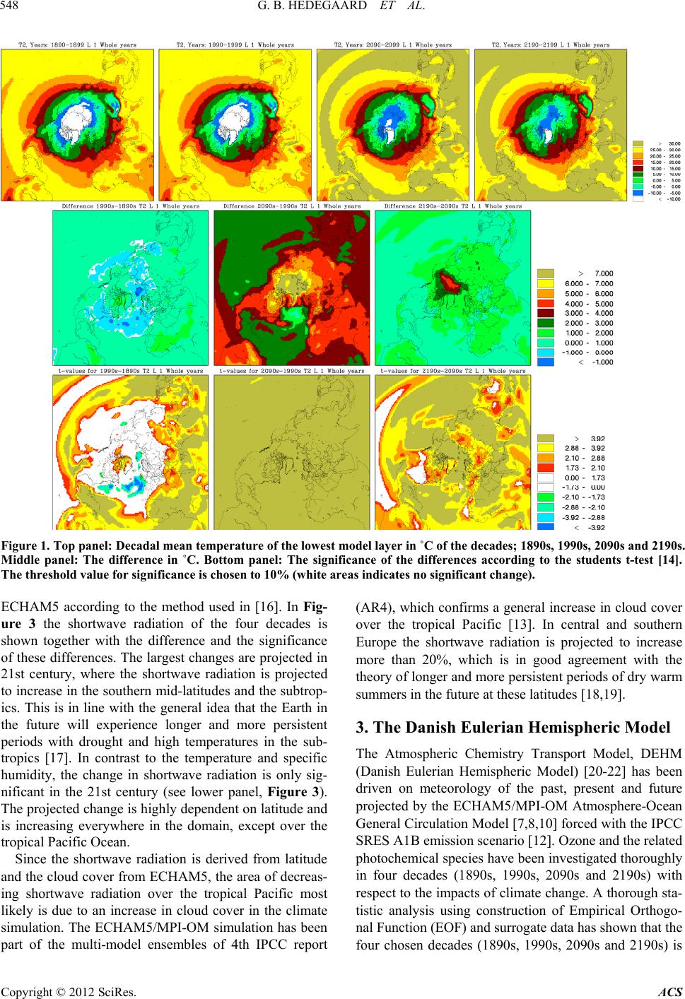

G. B. HEDEGAARD ET AL.
548
Figure 1. Top panel: Decadal mean temperature of the lowest model layer in ˚C of the decades; 1890s, 1990s, 2090s and 2190s.
Middle panel: The difference in ˚C. Bottom panel: The significance of the differences according to the students t-test [14].
The threshold value for significance is chosen to 10% (white areas indicates no significant change).
ECHAM5 according to the method used in [16]. In Fig-
ure 3 the shortwave radiation of the four decades is
shown together with the difference and the significance
of these differences. The largest changes are projected in
21st century, where the shortwave radiation is projected
to increase in the southern mid-latitudes and the subtrop-
ics. This is in line with the general idea that the Earth in
the future will experience longer and more persistent
periods with drought and high temperatures in the sub-
tropics [17]. In contrast to the temperature and specific
humidity, the change in shortwave radiation is only sig-
nificant in the 21st century (see lower panel, Figure 3).
The projected change is highly dependent on latitude and
is increasing everywhere in the domain, except over the
tropical Pacific Ocean.
(AR4), which confirms a general increase in cloud cover
over the tropical Pacific [13]. In central and southern
Europe the shortwave radiation is projected to increase
more than 20%, which is in good agreement with the
theory of longer and more persistent periods of dry warm
summers in the future at these latitudes [18,19].
3. The Danish Eulerian Hemispheric Model
The Atmospheric Chemistry Transport Model, DEHM
(Danish Eulerian Hemispheric Model) [20-22] has been
driven on meteorology of the past, present and future
projected by the ECHAM5/MPI-OM Atmosphere-Ocean
General Circulation Model [7,8,10] forced with the IPCC
SRES A1B emission scenario [12]. Ozone and the related
photochemical species have been investigated thoroughly
in four decades (1890s, 1990s, 2090s and 2190s) with
respect to the impacts of climate change. A thorough sta-
tistic analysis using construction of Empirical Orthogo-
nal Function (EOF) and surrogate data has shown that the
four chosen decades (1890s, 1990s, 2090s and 2190s) is
Since the shortwave radiation is derived from latitude
and the cloud cover from ECHAM5, the area of decreas-
ing shortwave radiation over the tropical Pacific most
likely is due to an increase in cloud cover in the climate
simulation. The ECHAM5/MPI-OM simulation has been
part of the multi-model ensembles of 4th IPCC report

G. B. HEDEGAARD ET AL. 549
Figure 2. Average decadal specific humidity in the lowest model layer in Kg·Kg–1. Setup the same as Figure 1.
representing the internal variability of the full 340-year
long period within a significance level of 10% [23]. The
performance of the full model system with ECHAM5/
MPI-OM model coupled to the DEHM model system has
been thoroughly tested in earlier studies [3,16].
In the current model setup, the model domain covers
slightly more than the Northern Hemisphere (see Figure
1). The horizontal grid has a resolution of 150 km × 150
km using a polar stereographic projection true at 60˚N.
Vertically the model consists of 20 unevenly distributed
layers defined on terrain following σ-levels extending up
to a height of approximately 16 km (100 hPa). Boundary
conditions for the model domain depend on the direction
of the wind, such that free boundary conditions are used
for sections where wind flows out of the domain. Con-
stant boundary conditions are used for sections of the
boundary where wind is flowing into the domain; in this
case, the boundary value is set to the annual average
background concentration. For ozone these are taken
from ozone soundings [24] and are the same for all simu-
lations in this study.
The chemistry scheme in DEHM is based on the Euro-
pean Monitoring and Evaluation Programme (EMEP)
scheme [25]. The model describes concentration fields of
58 chemical species, including secondary inorganic par-
ticles and 7 species representing primarily emitted par-
ticulate matter (PM2.5, PM10, TSP, sea-salt, fresh black
carbon, aged black carbon and organic carbon). A total of
122 chemical reactions are included. Wet and dry depo-
sition is parameterized similar to the EMEP model [25],
except for the dry deposition of species on water surfaces.
In this case, the deposition depends on the solubility of
the chemical specie and the wind speed (for further de-
tails see [26,27]). Details about the numerics can be found
in [20,28-30].
Emissions
The anthropogenic emissions that have been used as in-
put to the chemistry transport model DEHM have been
fixed at a year 2000 level to isolate the signal from cli-
mate change on air pollution. The emissions of the pri
mary pollutants consist of data from the Global Emis-
sions Inventory Activity (GEIA) [31], the Emission Da-
tabase for Global Atmospheric Research (EDGAR) [32]
both with global coverage, and the EMEP emissions [33]
covering Europe. The GEIA database includes natural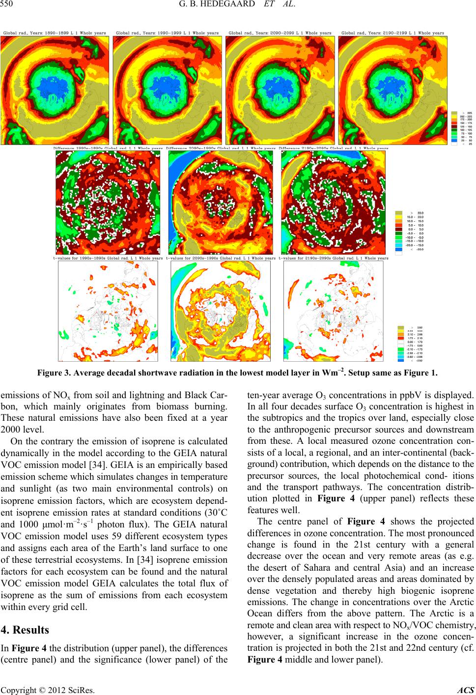

G. B. HEDEGAARD ET AL.
550
Figure 3. Average decadal shortwave radiation in the lowest model layer in Wm–2. Setup same as Figure 1.
emissions of NOx from soil and lightning and Black Car-
bon, which mainly originates from biomass burning.
These natural emissions have also been fixed at a year
2000 level.
On the contrary the emission of isoprene is calculated
dynamically in the model according to the GEIA natural
VOC emission model [34]. GEIA is an empirically based
emission scheme which simulates changes in temperature
and sunlight (as two main environmental controls) on
isoprene emission factors, which are ecosystem depend-
ent isoprene emission rates at standard conditions (30˚C
and 1000 μmol· m –2·s–1 photon flux). The GEIA natural
VOC emission model uses 59 different ecosystem types
and assigns each area of the Earth’s land surface to one
of these terrestrial ecosystems. In [34] isoprene emission
factors for each ecosystem can be found and the natural
VOC emission model GEIA calculates the total flux of
isoprene as the sum of emissions from each ecosystem
within every grid cell.
4. Results
In Figure 4 the distribution (upper panel), the differences
(centre panel) and the significance (lower panel) of the
ten-year average O3 concentrations in ppbV is displayed.
In all four decades surface O3 concentration is highest in
the subtropics and the tropics over land, especially close
to the anthropogenic precursor sources and downstream
from these. A local measured ozone concentration con-
sists of a local, a regional, and an inter-continental (back-
ground) contribution, which depends on the distance to the
precursor sources, the local photochemical cond- itions
and the transport pathways. The concentration distrib-
ution plotted in Figure 4 (upper panel) reflects these
features well.
The centre panel of Figure 4 shows the projected
differences in ozone concentration. The most pronounced
change is found in the 21st century with a general
decrease over the ocean and very remote areas (as e.g.
the desert of Sahara and central Asia) and an increase
over the densely populated areas and areas dominated by
dense vegetation and thereby high biogenic isoprene
emissions. The change in concentrations over the Arctic
Ocean differs from the above pattern. The Arctic is a
remote and clean area with respect to NOx/VOC chemistry,
however, a significant increase in the ozone concen-
tration is projected in both the 21st and 22nd century (cf.
Figure 4 middle and lower panel).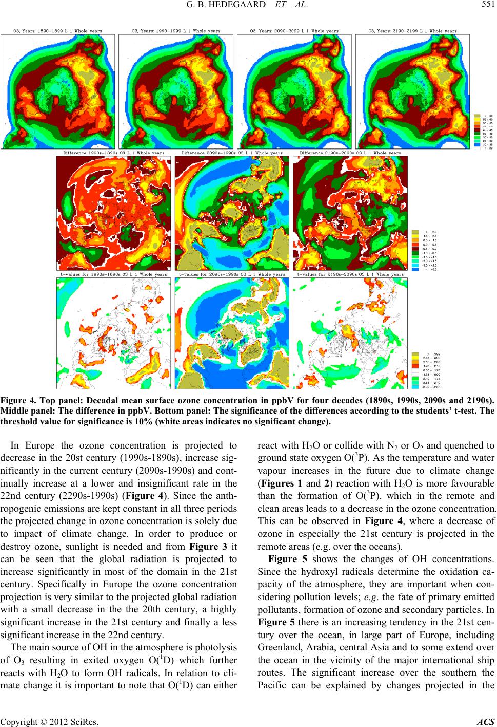

G. B. HEDEGAARD ET AL. 551
Figure 4. Top panel: Decadal mean surface ozone concentration in ppbV for four decades (1890s, 1990s, 2090s and 2190s).
Middle panel: The difference in ppbV. Bottom panel: The significance of the differences according to the students’ t-test. The
threshold value for significance is 10% (white areas indicates no significant change).
In Europe the ozone concentration is projected to
decrease in the 20st century (1990s-1890s), increase sig-
nificantly in the current century (2090s-1990s) and cont-
inually increase at a lower and insignificant rate in the
22nd century (2290s-1990s) (Figure 4). Since the anth-
ropogenic emissions are kept constant in all three periods
the projected change in ozone concentration is solely due
to impact of climate change. In order to produce or
destroy ozone, sunlight is needed and from Figure 3 it
can be seen that the global radiation is projected to
increase significantly in most of the domain in the 21st
century. Specifically in Europe the ozone concentration
projection is very similar to the projected global radiation
with a small decrease in the the 20th century, a highly
significant increase in the 21st century and finally a less
significant increase in the 22nd century.
The main source of OH in the atmosphere is photolysis
of O3 resulting in exited oxygen O(1D) which further
reacts with H2O to form OH radicals. In relation to cli-
mate change it is important to note that O(1D) can either
react with H2O or collide with N2 or O2 and quenched to
ground state oxygen O(3P). As the temperature and water
vapour increases in the future due to climate change
(Figures 1 and 2) reaction with H2O is more favourable
than the formation of O(3P), which in the remote and
clean areas leads to a decrease in the ozone concentration.
This can be observed in Figure 4, where a decrease of
ozone in especially the 21st century is projected in the
remote areas (e.g. over the oceans).
Figure 5 shows the changes of OH concentrations.
Since the hydroxyl radicals determine the oxidation ca-
pacity of the atmosphere, they are important when con-
sidering pollution levels; e.g. the fate of primary emitted
pollutants, formation of ozone and secondary particles. In
Figure 5 there is an increasing tendency in the 21st cen-
tury over the ocean, in large part of Europe, including
Greenland, Arabia, central Asia and to some extend over
the ocean in the vicinity of the major international ship
routes. The significant increase over the southern the
Pacific can be explained by changes projected in the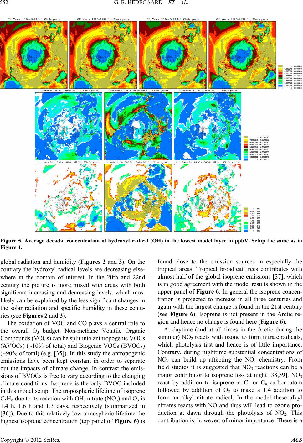

G. B. HEDEGAARD ET AL.
552
Figure 5. Average decadal concentration of hydroxyl radical (OH) in the lowest model layer in ppbV. Setup the same as in
Figure 4.
global radiation and humidity (Figures 2 and 3). On the
contrary the hydroxyl radical levels are decreasing else-
where in the domain of interest. In the 20th and 22nd
century the picture is more mixed with areas with both
significant increasing and decreasing levels, which most
likely can be explained by the less significant changes in
the solar radiation and specific humidity in these centu-
ries (see Figures 2 and 3).
The oxidation of VOC and CO plays a central role to
the overall O3 budget. Non-methane Volatile Organic
Compounds (VOCs) can be split into anthropogenic VOCs
(AVOCs) (~10% of total) and Biogenic VOCs (BVOCs)
(~90% of total) (e.g. [35]). In this study the antropogenic
emissions have been kept constant in order to separate
out the impacts of climate change. In contrast the emis-
sions of BVOCs is free to vary according to the changing
climate conditions. Isoprene is the only BVOC included
in this model setup. The tropospheric lifetime of isoprene
C5H8 due to its reaction with OH, nitrate (NO3) and O3 is
1.4 h, 1.6 h and 1.3 days, respectively (summarized in
[36]). Due to this relatively low atmospheric lifetime the
highest isoprene concentration (top panel of Figure 6) is
found close to the emission sources in especially the
tropical areas. Tropical broadleaf trees contributes with
almost half of the global isoprene emissions [37], which
is in good agreement with the model results shown in the
upper panel of Figure 6. In general the isoprene concen-
tration is projected to increase in all three centuries and
again with the largest change is found in the 21st century
(see Figure 6). Isoprene is not present in the Arctic re-
gion and hence no change is found here (Figure 6).
At daytime (and at all times in the Arctic during the
summer) NO2 reacts with ozone to form nitrate radicals,
which photolysis fast and hence is of little importance.
Contrary, during nighttime substantial concentrations of
NO2 can build up affecting the NOx chemistry. From
field studies it is suggested that NO3 reactions can be a
major contributor to isoprene loss at night [38,39]. NO3
react by addition to isoprene at C1 or C4 carbon atom
followed by addition of O2 to make a 1.4 addition to
form an alkyl nitrate radical. In the model these alkyl
nitrates reacts with NO and thus will lead to ozone pro-
duction at dawn through the photolysis of NO2. This
contribution is, however, of mnor importance. There is a i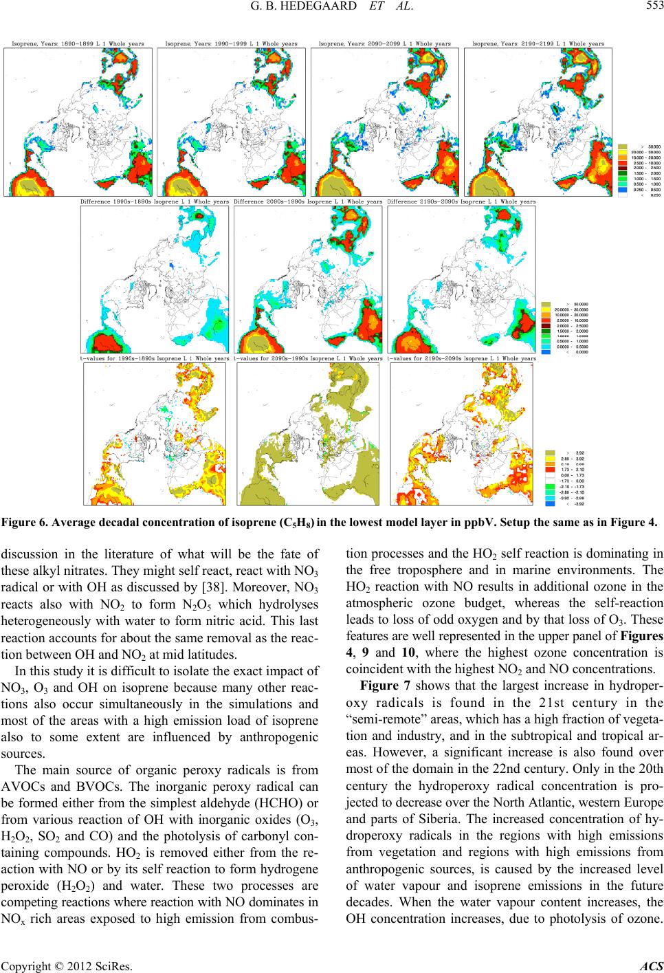

G. B. HEDEGAARD ET AL. 553
Figure 6. Average decadal concentration of isoprene (C5H8) in the lowest model layer in ppbV. Setup the same as in Figure 4.
discussion in the literature of what will be the fate of
these alkyl nitrates. They might self react, react with NO3
radical or with OH as discussed by [38]. Moreover, NO3
reacts also with NO2 to form N2O5 which hydrolyses
heterogeneously with water to form nitric acid. This last
reaction accounts for about the same removal as the reac-
tion between OH and NO2 at mid latitudes.
In this study it is difficult to isolate the exact impact of
NO3, O3 and OH on isoprene because many other reac-
tions also occur simultaneously in the simulations and
most of the areas with a high emission load of isoprene
also to some extent are influenced by anthropogenic
sources.
The main source of organic peroxy radicals is from
AVOCs and BVOCs. The inorganic peroxy radical can
be formed either from the simplest aldehyde (HCHO) or
from various reaction of OH with inorganic oxides (O3,
H2O2, SO2 and CO) and the photolysis of carbonyl con-
taining compounds. HO2 is removed either from the re-
action with NO or by its self reaction to form hydrogene
peroxide (H2O2) and water. These two processes are
competing reactions where reaction with NO dominates in
NOx rich areas exposed to high emission from combus-
tion processes and the HO2 self reaction is dominating in
the free troposphere and in marine environments. The
HO2 reaction with NO results in additional ozone in the
atmospheric ozone budget, whereas the self-reaction
leads to loss of odd oxygen and by that loss of O3. These
features are well represented in the upper panel of Figures
4, 9 and 10, where the highest ozone concentration is
coincident with the highest NO2 and NO concentrations.
Figure 7 shows that the largest increase in hydroper-
oxy radicals is found in the 21st century in the
“semi-remote” areas, which has a high fraction of vegeta-
tion and industry, and in the subtropical and tropical ar-
eas. However, a significant increase is also found over
most of the domain in the 22nd century. Only in the 20th
century the hydroperoxy radical concentration is pro-
jected to decrease over the North Atlantic, western Europe
and parts of Siberia. The increased concentration of hy-
droperoxy radicals in the regions with high emissions
from vegetation and regions with high emissions from
anthropogenic sources, is caused by the increased level
of water vapour and isoprene emissions in the future
decades. When the water vapour content increases, the
OH concentration increases, due to photolysis of ozone.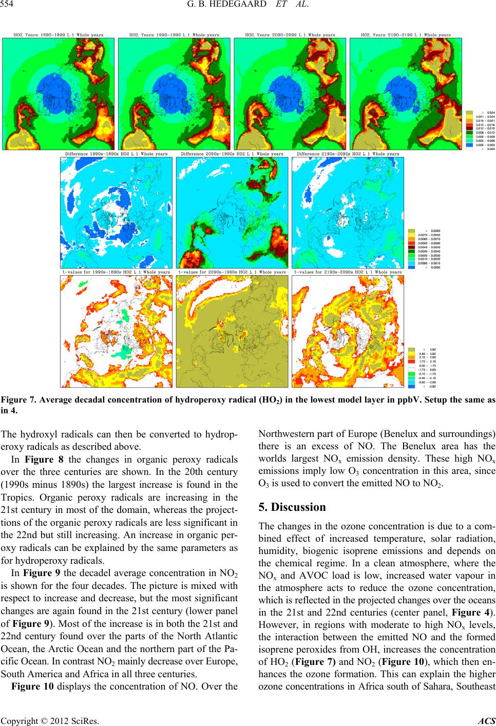

G. B. HEDEGAARD ET AL.
554
Figure 7. Average decadal concentration of hydroperoxy radical (HO2) in the lowest model layer in ppbV. Setup the same as
in 4.
The hydroxyl radicals can then be converted to hydrop-
eroxy radicals as described above.
In Figure 8 the changes in organic peroxy radicals
over the three centuries are shown. In the 20th century
(1990s minus 1890s) the largest increase is found in the
Tropics. Organic peroxy radicals are increasing in the
21st century in most of the domain, whereas the project-
tions of the organic peroxy radicals are less significant in
the 22nd but still increasing. An increase in organic per-
oxy radicals can be explained by the same parameters as
for hydroperoxy radicals.
In Figure 9 the decadel average concentration in NO2
is shown for the four decades. The picture is mixed with
respect to increase and decrease, but the most significant
changes are again found in the 21st century (lower panel
of Figure 9). Most of the increase is in both the 21st and
22nd century found over the parts of the North Atlantic
Ocean, the Arctic Ocean and the northern part of the Pa-
cific Ocean. In contrast NO2 mainly decrease over Europe,
South America and Africa in all three centuries.
Figure 10 displays the concentration of NO. Over the
Northwestern part of Europe (Benelux and surroundings)
there is an excess of NO. The Benelux area has the
worlds largest NOx emission density. These high NOx
emissions imply low O3 concentration in this area, since
O3 is used to convert the emitted NO to NO2.
5. Discussion
The changes in the ozone concentration is due to a com-
bined effect of increased temperature, solar radiation,
humidity, biogenic isoprene emissions and depends on
the chemical regime. In a clean atmosphere, where the
NOx and AVOC load is low, increased water vapour in
the atmosphere acts to reduce the ozone concentration,
which is reflected in the projected changes over the oceans
in the 21st and 22nd centuries (center panel, Figure 4).
However, in regions with moderate to high NOx levels,
the interaction between the emitted NO and the formed
isoprene peroxides from OH, increases the concentration
of HO2 (Figure 7) and NO2 (Figure 10), which then en-
hances the ozone formation. This can explain the higher
ozone concentrations in Africa south of Sahara, Southeast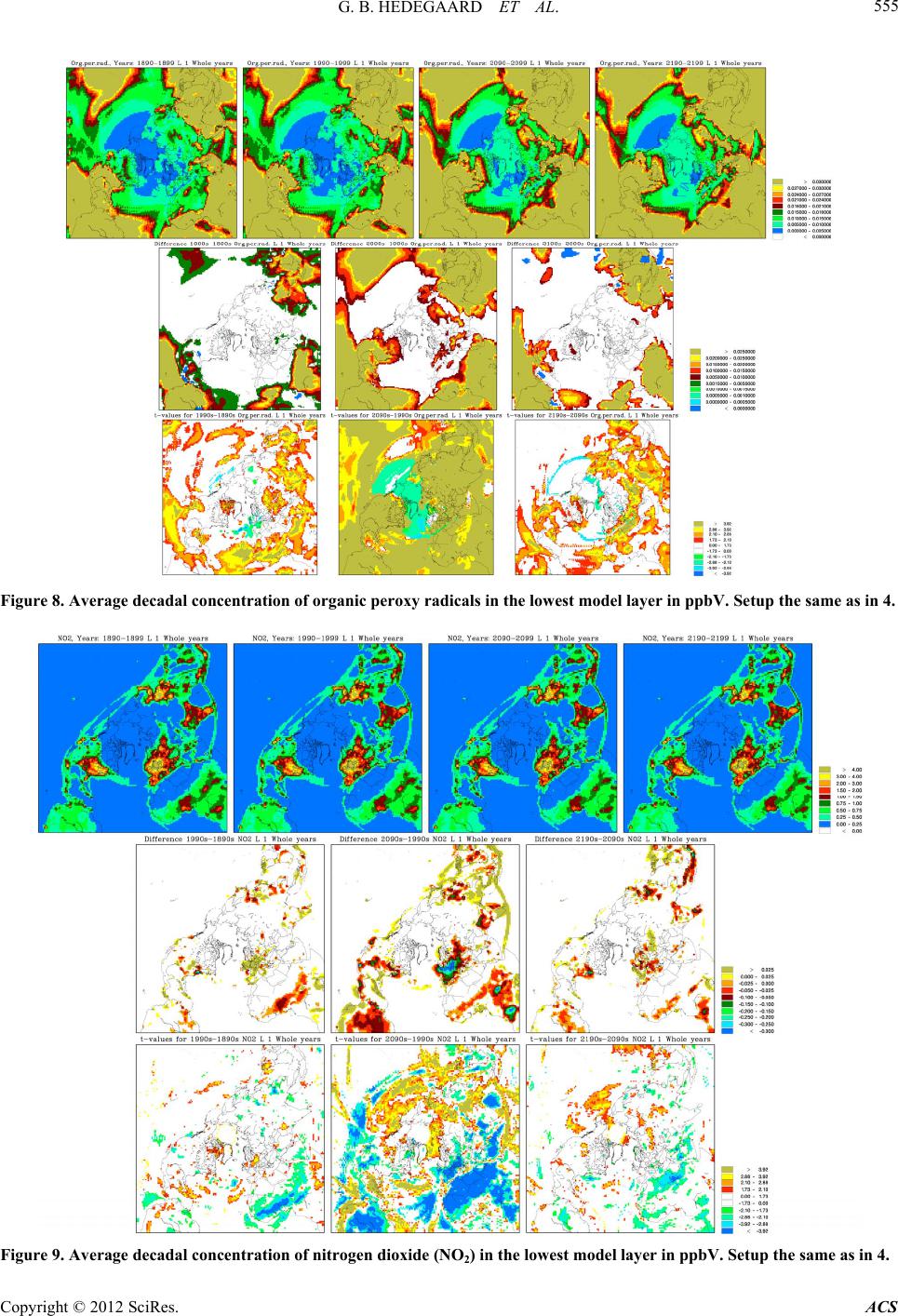

G. B. HEDEGAARD ET AL. 555
Figure 8. Average decadal concentration of organic peroxy radicals in the lowest model layer in ppbV. Setup the same as in 4.
Figure 9. Average decadal concentration of nitrogen dioxide (NO2) in the lowest model layer in ppbV. Setup the same as in 4.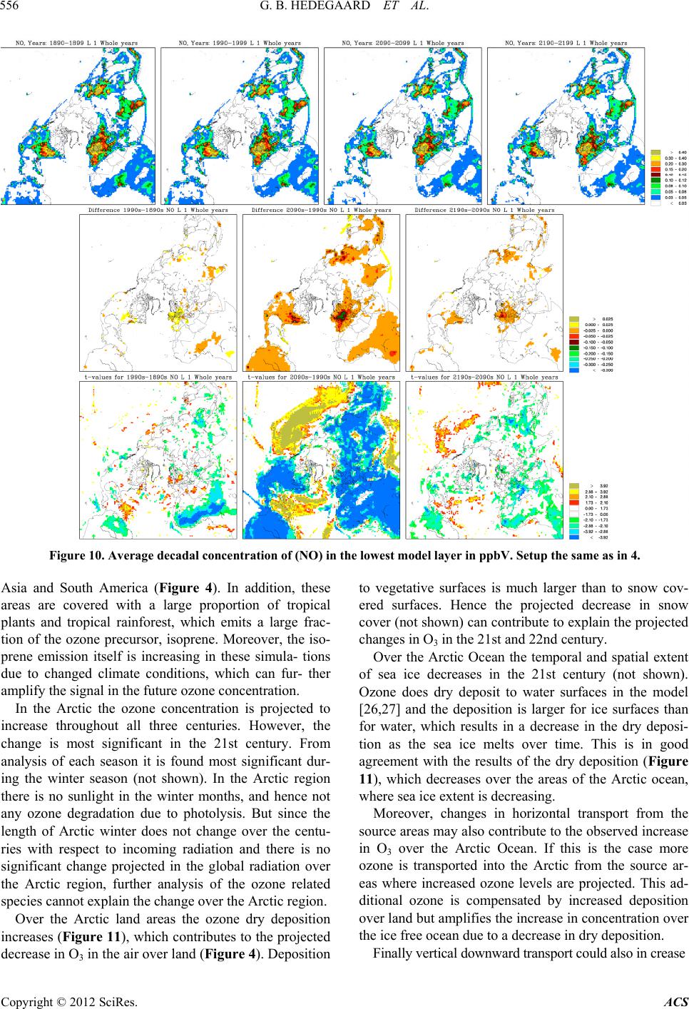

G. B. HEDEGAARD ET AL.
556
Figure 10. Average decadal concentration of (NO) in the lowest model layer in ppbV. Setup the same as in 4.
Asia and South America (Figure 4). In addition, these
areas are covered with a large proportion of tropical
plants and tropical rainforest, which emits a large frac-
tion of the ozone precursor, isoprene. Moreover, the iso-
prene emission itself is increasing in these simula- tions
due to changed climate conditions, which can fur- ther
amplify the signal in the future ozone concentration.
In the Arctic the ozone concentration is projected to
increase throughout all three centuries. However, the
change is most significant in the 21st century. From
analysis of each season it is found most significant dur-
ing the winter season (not shown). In the Arctic region
there is no sunlight in the winter months, and hence not
any ozone degradation due to photolysis. But since the
length of Arctic winter does not change over the centu-
ries with respect to incoming radiation and there is no
significant change projected in the global radiation over
the Arctic region, further analysis of the ozone related
species cannot explain the change over the Arctic region.
Over the Arctic land areas the ozone dry deposition
increases (Figure 11), which contributes to the projected
decrease in O3 in the air over land (Figure 4). Deposition
to vegetative surfaces is much larger than to snow cov-
ered surfaces. Hence the projected decrease in snow
cover (not shown) can contribute to explain the projected
changes in O3 in the 21st and 22nd century.
Over the Arctic Ocean the temporal and spatial extent
of sea ice decreases in the 21st century (not shown).
Ozone does dry deposit to water surfaces in the model
[26,27] and the deposition is larger for ice surfaces than
for water, which results in a decrease in the dry deposi-
tion as the sea ice melts over time. This is in good
agreement with the results of the dry deposition (Figure
11), which decreases over the areas of the Arctic ocean,
where sea ice extent is decreasing.
Moreover, changes in horizontal transport from the
source areas may also contribute to the observed increase
in O3 over the Arctic Ocean. If this is the case more
ozone is transported into the Arctic from the source ar-
eas where increased ozone levels are projected. This ad-
ditional ozone is compensated by increased deposition
over land but amplifies the increase in concentration over
the ice free ocean due to a decrease in dry deposition.
Finally vertical downward transport could also in crease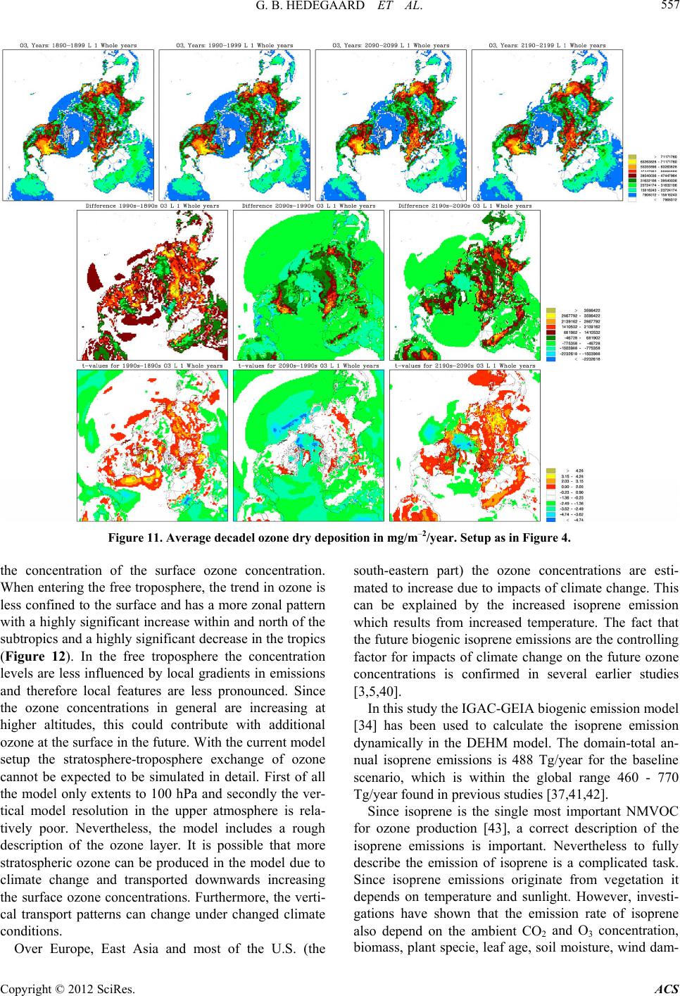

G. B. HEDEGAARD ET AL. 557
Figure 11. Average decadel ozone dry deposition in mg/m–2/year. Setup as in Figure 4.
the concentration of the surface ozone concentration.
When entering the free troposphere, the trend in ozone is
less confined to the surface and has a more zonal pattern
with a highly significant increase within and north of the
subtropics and a highly significant decrease in the tropics
(Figure 12). In the free troposphere the concentration
levels are less influenced by local gradients in emissions
and therefore local features are less pronounced. Since
the ozone concentrations in general are increasing at
higher altitudes, this could contribute with additional
ozone at the surface in the future. With the current model
setup the stratosphere-troposphere exchange of ozone
cannot be expected to be simulated in detail. First of all
the model only extents to 100 hPa and secondly the ver-
tical model resolution in the upper atmosphere is rela-
tively poor. Nevertheless, the model includes a rough
description of the ozone layer. It is possible that more
stratospheric ozone can be produced in the model due to
climate change and transported downwards increasing
the surface ozone concentrations. Furthermore, the verti-
cal transport patterns can change under changed climate
conditions.
Over Europe, East Asia and most of the U.S. (the
south-eastern part) the ozone concentrations are esti-
mated to increase due to impacts of climate change. This
can be explained by the increased isoprene emission
which results from increased temperature. The fact that
the future biogenic isoprene emissions are the controlling
factor for impacts of climate change on the future ozone
concentrations is confirmed in several earlier studies
[3,5,40].
In this study the IGAC-GEIA biogenic emission model
[34] has been used to calculate the isoprene emission
dynamically in the DEHM model. The domain-total an-
nual isoprene emissions is 488 Tg/year for the baseline
scenario, which is within the global range 460 - 770
Tg/year found in previous studies [37,41,42].
Since isoprene is the single most important NMVOC
for ozone production [43], a correct description of the
isoprene emissions is important. Nevertheless to fully
describe the emission of isoprene is a complicated task.
Since isoprene emissions originate from vegetation it
depends on temperature and sunlight. However, investi-
gations have shown that the emission rate of isoprene
also depend on the ambient CO2 and O3 concentration,
biomass, plant specie, leaf age, soil moisture, wind dam-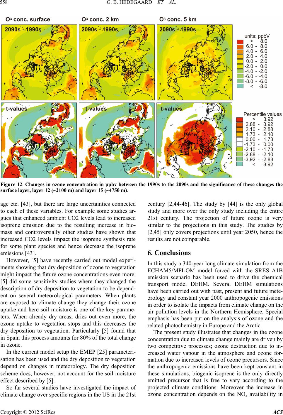

G. B. HEDEGAARD ET AL.
558
Figure 12. Changes in ozone concentration in ppbv between the 1990s to the 2090s and the significance of these changes the
surface layer, layer 12 (~2100 m) and layer 15 (~4750 m).
age etc. [43], but there are large uncertainties connected
to each of these variables. For example some studies ar-
gues that enhanced ambient CO2 levels lead to increased
isoprene emission due to the resulting increase in bio-
mass and controversially other studies have shown that
increased CO2 levels impact the isoprene synthesis rate
for some plant species and hence decrease the isoprene
emissions [43].
However, [5] have recently carried out model experi-
ments showing that dry deposition of ozone to vegetation
might impact the future ozone concentrations even more.
[5] did some sensitivity studies where they changed the
description of dry deposition to vegetation to be depend-
ent on several meteorological parameters. When plants
are exposed to climate change they change their ozone
uptake and here soil moisture is one of the key parame-
ters. When already dry areas, dries out even more, the
ozone uptake to vegetation stops and this decreases the
dry deposition to vegetation. Particularly [5] found that
in Spain this process amounts for 80% of the total change
in ozone.
In the current model setup the EMEP [25] parameteri-
sation has been used and the dry deposition to vegetation
depend on changes in meteorology. The dry deposition
scheme does, however, not account for the soil moisture
effect described by [5].
So far several studies have investigated the impact of
climate change over specific regions in the US in the 21st
century [2,44-46]. The study by [44] is the only global
study and more over the only study including the entire
21st century. The projection of future ozone is very
similar to the projections in this study. The studies by
[2,45] only covers projections until year 2050, hence the
results are not comparable.
6. Conclusions
In this study a 340-year long climate simulation from the
ECHAM5/MPI-OM model forced with the SRES A1B
emission scenario has been used to drive the chemical
transport model DEHM. Several DEHM simulations
have been carried out with past, present and future mete-
orology and constant year 2000 anthropogenic emissions
in order to isolate the impacts from climate change on the
air pollution levels in the Northern Hemisphere. Special
emphasis has been put on the analysis of ozone and the
related photochemistry in Europe and the Arctic.
The present study illustrates that changes in the ozone
concentration due to climate change mainly are driven by
two competitive processes; ozone destruction due to in-
creased water vapour in the atmosphere and ozone for-
mation due to increased levels of ozone precursors. Since
the anthropogenic emissions have been kept constant in
these simulations, biogenic isoprene is the only directly
emitted precursor that is free to vary according to the
projected climate conditions. Moreover the increase in
ozone concentration depends on the NOx availability in

G. B. HEDEGAARD ET AL. 559
the boundary layer and the future ozone concentration is
projected to increase significantly in urban and semi-
remote areas and to decrease significantly in the remote
areas. In the free troposphere the effect from increased
water vapour dominates in the tropics while the effect
from increased isoprene and changes in transport domi-
nates at high latitudes.
These results show a close relation between the tem-
perature change and the future ozone concentration. The
two parameters are not directly connected but are related
through a wide range of interacting processes. From the
climate simulation it is known that the largest change in
temperature is projected to happen in the 21st century
and the same is true for ozone, isoprene, NOx and OH. In
the 20th century the temperature change is relatively
small and in some areas decreasing and other areas in-
creasing. The same patterns are seen in most chemical
species e.g. in the O3 concentration. In the 22nd century
the trends are the same as in the 21st century, but the rate
of change decreases for all parameters, which is in good
agreement with the constant forcing in the applied cli-
mate simulation (constant A1B year-2100 level emission
throughout the 22nd century).
Surface ozone is of great importance since high ozone
concentrations can have impacts on both humans and
nature. This study has shown that at the surface level the
background ozone concentration will decrease during the
21st and the 22nd century. In contrast local ozone in the
source areas of precursors (both anthropogenic and bio-
genic) will increase significantly due to climate change
alone. In the free troposphere the ozone concentration
will in general increase, except in the tropics where a
significant decrease is found. Over the Arctic Ocean a
significant increase in surface ozone is found in the fu-
ture, which can be explained by increased input from the
source areas. Moreover, decreased dry deposition of
ozone due to increased sea ice and increased import from
higher levels can support the projected increase in future
surface level ozone in the Arctic region.
Ozone in the atmosphere affects not only the human
health and nature. It is also a significant short-lived
greenhouse gas in the atmosphere. Today most atmos-
pheric climate models have lower resolution than ACTMs
and a more simplified descriptions of the atmospheric
physical and chemical processes and therefore account
poorly for the feedback from atmospheric chemistry to
the climate system. The increase in ozone concentrations
in large parts of the upper troposphere could have sig-
nificant radiative effect, which is not yet accounted for in
climate models. To include this and similar chemical
feedback effects in the atmosphere, online model or ex-
tensive Earth system models are needed. Nevertheless,
CTM studies like the present are still necessary in order
to study in detail the individual chemical and physical
processes in the atmosphere.
7. Acknowledgements
This work was partly funded by the Centre for Energy,
Environment and Health (CEEH), financed by The Dan-
ish Strategic Research Program on Sustainable Energy
under contract no 2104-06-0027 (www.ceeh.dk).
REFERENCES
[1] S. L. Wu, L. J. Mickley, D. J. Jacob, D. Rind and D. G.
Streets, “Effects of 2000-2050 Changes in Climate and
Emissions on Global Tropospheric Ozone and the Pol-
icy-Relevant Background Ozone in the United States,”
Journal of Geophysical Research, Vol. 113, 2008, Article
ID: D18312.
[2] P. N. Racherla and P. J. Adams, “The Response of Surface
Ozone to Climate Change over Eastern United States,”
Atmospheric Chemistry and Physics, Vol. 8, No. 4, 2008,
pp. 871-885. doi:10.5194/acp-8-871-2008
[3] G. B. Hedegaard, J. Brandt, J. H. Christensen, L. M.
Frohn, C. Geels, K. M. Hansen and M. Stendel, “Impacts
of Climate Change on Air Pollution Levels in the North-
ern Hemisphere with Special Focus on Europe and the
Arctic,” Atmospheric Chemistry and Physics, Vol. 8, No.
12, 2008, pp. 3337-3367. doi:10.5194/acp-8-3337-2008
[4] E. Katragkou, P. Zanis, I. Tegoulias, D. Melas, I. Kiout-
sioukis, B. C. Krger, P. Huszar, T. Halenka and S.
Rauscher, “Decadal Regional Air Quality Simulations
over Europe in Present Climate: Near Surface Ozone Sen-
sitivity to External Meteorological Forcing,” Atmospheric
Chemistry and Physics, Vol. 10, 2010, pp. 11805-11821.
[5] C. Andersson and M. Engardt, “European Ozone in a Fu-
ture Climate: Importance of Changes in Dry Deposition
and Isoprene Emissions,” Journal of Geophysical Re-
search, Vol. 115, No. D2, 2010, Article ID: D02303.
doi:10.1029/2008JD011690
[6] J. Langner, M. Engardt, A. Baklanov, J. Christensen, M.
Gauss, C. Geels, G. B. Hedegaard, R. Nuterman, D.
Simpson, J. Soares, M. Sofiev, P. Wind and A. Zakey, “A
Multi-Model Study of Impacts of Climate Change on Sur-
face Ozone in Europe,” Atmospheric Chemistry and Phys-
ics, Vol. 12, No. 2, 2012, pp. 4901-4939.
doi:10.5194/acpd-12-4901-2012
[7] E. Roeckner, G. Bauml, L. Bonaventura, R. Brokopf, M.
Esch, M. Giorgetta, S. Hagemann, I. Kirchner, L. Korn-
blueh, E. Manzini, A. Rhodin, U. Schlese, U. Schul-
zweida and A. Tompkins, “The Atmospheric General
Circulation Model ECHAM5, Part I,” Max-Planck-Insti-
tute für Meteorologie, Hamburg, 2003.
[8] E. Roeckner, R. Brokopf, M. Esch, M. Giorgetta, S.
Hagemann, E. Kornblueh, L. Manzini, U. Schlese and U.
Schulzweida, “Sensitivity of Simulated Climate to Hori-
zontal and Vertical Resolution in the ECHAM5 Atmos-
phere Model,” Journal of Climate, Vol. 19, No. 16, 2006,
pp. 3771-3791. doi:10.1175/JCLI3824.1
[9] S. J. Marsland, H. Haak, J. H. Jungclaus, M. Latif and F.
Roske, “The Max-Planck-Institute Global Ocean/Sea Ice

G. B. HEDEGAARD ET AL.
560
Model with Orthogonal Curvilinear Coordinates,” Ocean
Modelling, Vol. 5, No. 2, 2003, pp. 91-127.
doi:10.1016/S1463-5003(02)00015-X
[10] W. May, “Climatic Changes Associated with a Global 2
Degrees C-Stabilization Scenario Simulated by the EC
HAM5/MPI-OM Coupled Climate Model,” Climate Dy-
namics, Vol. 31, No. 2-3, 2008, pp. 283-313.
doi:10.1007/s00382-007-0352-8
[11] J. H. Jungclaus, N. Keenlyside, M. Botzet, H. Haak, J. J.
Luo, M. Latif, J. Marotzke, U. Mikolajewicz and E.
Roeckner, “Ocean Circulation and Tropical Variability in
the Coupled Model ECHAM5/MPI-OM,” Journal of Cli-
mate, Vol. 19, No. 16, 2006, pp. 3952-3972.
doi:10.1175/JCLI3827.1
[12] N. Nakicenovic, J. Alcamo, G. Davis, B. de Vries, J.
Fenhann, S. Gaffin, K. Gregory, A. Grbler, T. Jung, T.
Kram, E. L. Rovere, L. Michaelis, S. Mori, T. Morita, W.
Pepper, H. Pitcher, L. Price, K. Riahi, A. Roehrl, H.-H.
Rogner, A. Sankovski, M. Schlesinger, P. Shukla, S.
Smith, R. Swart, S. van Rooijen, N. Victor and Z. Dadi,
“Special Report on Emission Scenarios: A Special Report
of Working Group III of the Intergovernmental Panel on
Climate Change,” Cambridge University Press, New York,
2000.
[13] G. A. Meehl, T. F. Stocker, W. D. Collins, P. Friedling-
stein, A. T. Gaye, J. M. Gregory, A. Kitoh, R. Knutti, J.
M. Murphy, A. Noda, S. C. B. Raper, I. G. Watterson, A.
J. Weaver and Z.-C. Zhao, “Climate Change 2007: The
Physical Science Basis,” In: Contribution of Working
Group I to the Fourth Assessment Report of the Intergov-
ernmental Panel on Climate Change Global Climate
Projections, Cambridge University Press, Cambridge and
New York, 2007, pp. 747-846.
[14] M. R. Spiegel, “Schaum’s Outline of Theory and Prob-
lems of Statistics,” 2nd Edition, McGraw-Hill, New York,
1992.
[15] H. Goosse, P. Y. Barriat, W. Lefebvre, M. F. Loutre and
V. Zunz, “Introduction to Climate Dynamics and Climate
Modelling,” 2009. http://stratus.astr.ucl.ac.be/textbook/
[16] G. B. Hedegaard, “Impacts of Climate Change on Air
Pollution Levels in the Northern Hemisphere,” Technical
Report 240, National Environmental Research Institute,
Roskilde, 2007. www.dmu.dk
[17] J. H. Christensen, C. Hewitt, A. Busuioc, A. Chen, X.
Gao, I. Held, R. Jones, R. K. Kolli, W.-T. Kwon, R. La-
prise, V. Magaa Rueda, L. Mearns, C. G. Menendez, J.
Risnen, A. Rinke, A. Sarr and P. Whetton, “Climate
Change 2007: The Physical Science Basis,” In: Contribu-
tion of Working Group I to the Fourth Assessment Report
of the Intergovernmental Panel on Climate Change Re-
gional Climate Projections, Cambridge University Press,
Cambridge, 2007, pp. 847-940.
[18] R. Vautard and D. Hauglustaine, “Impact of Global Cli-
mate Change on Regional Air Quality: Introduction to the
Thematic Issue,” Comptes Rendus Geoscience, Vol. 339,
No. 11-12, 2007, pp. 703-708.
doi:10.1016/j.crte.2007.08.012
[19] P. A. Stott, D. A. Stone and M. R. Allen, “Human Con-
tribution to the European Heatwave of 2003,” Nature, Vol.
432, 2004, pp. 610-614. doi:10.1038/nature03089
[20] J. H. Christensen, “The Danish Eulerian Hemispheric
Model—A Three-Dimensional Air Pollution Model Used
for the Arctic,” Atmospheric Environment, Vol. 31, No.
24, 1997, pp. 4169-4191.
doi:10.1016/S1352-2310(97)00264-1
[21] L. M. Frohn, “A Study of Long-Term Highresolution Air
Pollution Modelling,” Ph.D. Dissertation, University of
Copenhagen and National Environmental Research Insti-
tute, Copenhagen, 2004.
[22] J. Brandt, J. D. Silver, L. M. Frohn, C. Geels, A. Gross, A.
B. Hansen, K. M. Hansen, G. B. Hedegaard, C. A. Skjøth,
H. Villadsen, A. Zare and J. H. Christensen, “An Inte-
grated Model Study for Europe and North America Using
the Danish Eulerian Hemispheric Model with Focus on
Intercontinental Transport of Air Pollution,” Atmospheric
Environment, Vol. 53, 2012, pp. 156-176.
doi:10.1016/j.atmosenv.2012.01.011
[23] G. B. Hedegaard, “Future Air Pollution Levels in the
Northern Hemisphere—Sensitivity to Climate Change
and Projected Emissions,” Ph.D. Thesis, Aarhus Univer-
sity, Aarhus, 2011.
[24] J. A. Logan, “An Analysis of Ozonesonde Data for the
Troposphere: Recommendations for Testing 3-D Models
and Development of a Gridded Climatology for Tropo-
spheric Ozone,” Journal of Geophysical Research, Vol.
104, No. D13, 1999, pp. 115-116.
doi:10.1029/1998JD100096
[25] D. Simpson, H. Fagerli, J. Jonson, S. Tsyro, P. Wind and
J.-P. Touvinen, “Transboundary Acidification, Eutrophi-
cation and Ground Level Ozone in Europe, Part I,” Nor-
wegian Meteorological Institute, Unified EMEP Model
description EMEP MSC-W, Oslo, 2003.
[26] W. A. H. Asman, L. L. Sensen, R. Berkowicz, K. Granby,
H. Nielsen, B. Jensen, E. Runge, C. Lykkelund, S. E.
Gryning and A. M. Sempreviva, “Dry Deposition Proc-
esses,” Marine Research 35, Danish Environmental Pro-
tection Agency, Copenhagen, 1994.
[27] O. Hertel, J. Christensen, E. H. Runge, W. A. H. Asman,
R. Berkowicz and M. F. Hovmand, “Development and
Testing of a New Variable Scale Pollution Model—
ACDEP,” Atmospheric Environment, Vol. 29, No. 11,
1995, pp. 1267-1290. doi:10.1016/1352-2310(95)00067-9
[28] L. M. Frohn, J. H. Christensen, J. Brandt and O. Hertel,
“Development of a High Resolution Integrated Nested
Model for Studying Air Pollution in Denmark,” Physics
and Chemistry of the Earth, Vol. 26, Part B, 2001, pp.
769-774.
[29] L. M. Frohn, J. H. Christensen and J. Brandt, “Develop-
ment and Testing of Numerical Methods for Two-Way
Nested Air Pollution Modelling,” Physics and Chemistry
of the Earth, Vol. 27, No. 35, 2002, pp. 1487-1494.
doi:10.1016/S1474-7065(02)00151-1
[30] L. M. Frohn, J. H. Christensen and J. Brandt, “Develop-
ment of a High-Resolution Nested Air Pollution Model:
The Numerical Approach,” Journal of Computational
Physics, Vol. 179, No. 1, 2002, pp. 68-94.
doi:10.1006/jcph.2002.7036
[31] T. Graedel, T. Bates, A. Bouwman, D. Cunnold, J. Dignon,

G. B. HEDEGAARD ET AL.
561
I. Fung, D. Jacob, B. Lamb, J. Logan, G. Marland, P.
Middleton, J. Pacyna, M. Placet and C. Veldt, “A Com-
pilation of Inventories of Emissions to the Atmosphere,”
Global Biogeochemical Cycles, Vol. 7, No. 1, 1993, pp.
1-26. doi:10.1029/92GB02793
[32] J. Olivier, A. Bouwman, C. van der Maas, J. Berdowski,
C. Veldt, J. Bloos, A. Visschedijk, P. Zandveld and J.
Haverlag, “Description of EDGAR Version 2.0: A Set of
Global Emission Inventories of Greenhouse Gases and
Ozone-Depleting Substances for All Anthropogenic and
Most Natural Sources on a Per Country Basis and on 1
Degree × 1 Degree Grid,” National Institute for Public
Health and the Environment (RIVM), Bilthoven, 1996.
[33] V. Vestreng, “Emission Data Reported to UNECE/
EMEP: Evaluation of the Spatial Distribution of Emis-
sion,” MSC-W Status Report, Meteorological Synthesiz-
ing Centre—West, Oslo, 2001.
[34] A. Guenther, C. Hewitt, D. Erickson, R. Fall, C. Geron, T.
Graedel, P. Harley, L. Klinger, M. Lerdau, W. McKay, T.
Pierce, B. Scholes, R. Steinbrecher, R. Tallamraju, J.
Taylor and P. Zimmerman, “A Global-Model of Natural
Volatile Organic-Compound Emissions,” Journal of Geo-
physical Research, Vol. 100, No. D5, 1995, pp. 8873-
8892. doi:10.1029/94JD02950
[35] A. H. Goldstein and I. E. Galbally, “Known and Unex-
plored Organic Constituents in the Earths Atmosphere,”
Environmental Science & Technology, Vol. 41, No. 5,
2007, pp. 1514-1521. doi:10.1021/es072476p
[36] G. B. Hedegaard, “Air Pollution—From a Local to a
Global Perspective,” Polyteknisk Forlag, Lyngby, 2009,
pp. 163-174.
[37] A. Guenther, T. Karl, P. Harley, C. Wiedinmyer, P. I.
Palmer and C. Geron, “Estimates of Global Terrestrial
Isoprene Emissions Using MEGAN (Model of Emissions
of Gases and Aerosols from Nature),” Atmospheric
Chemistry and Physics, Vol. 6, No. 11, 2006, pp. 3181-
3210. doi:10.5194/acp-6-3181-2006
[38] A. W. Rollins, A. Kiendler-Scharr, J. L. Fry, T. Brauers,
S. S. Brown, H.-P. Dorn, W. P. Dube, H. Fuchs, A. Men-
sah, T. F. Mentel, F. Rohrer, R. Tillmann, R. Wegener, P.
J. Wooldridge and R. C. Cohen, “Isoprene Oxidation by
Nitrate Radical: Alkyl Nitrate and Secondary Organic
Aerosol Yields,” Atmospheric Chemistry and Physics,
Vol. 9, No. 18, 2009, pp. 6685-6703.
doi:10.5194/acp-9-6685-2009
[39] H. Skov, J. Hjorth, C. Lohse, N. R. Jensen and G. Restelli,
“Products and Mechanisms of the Reactions of the Nitrate
Radical (NO3) with Isoprene, 1,3-Butadiene and 2,3-Di-
methyl-1,3-Butadiene in Air,” Atmospheric Environment:
Part A. General Topics, Vol. 26, No. 15, 1992, pp. 2771-
2783. doi:10.1016/0960-1686(92)90015-D
[40] Y. F. Lam, J. S. Fu and L. J. Mickley, “Impacts of Future
Climate Change and Effects of Biogenic Emissions on
Surface Ozone and Particulate Matter Concentrations in
the United States,” Atmospheric Chemistry and Physics,
Vol. 11, No. 10, 2011, pp. 4789-4806.
doi:10.5194/acp-11-4789-2011
[41] A. Arneth, R. K. Monson, G. Schurgers, U. Niinemets
and P. I. Palmer, “Why Are Estimates of Global Terres-
trial Isoprene Emissions So Similar (and Why Is This Not
so for Monoterpenes)?” Atmospheric Chemistry and Phy-
sics, Vol. 8, No. 16, 2008, pp. 4605-4620.
[42] K. Ashworth, O. Wild and C. N. Hewitt, “Sensitivity of
Isoprene Emissions Estimated Using Megan to the Time
Resolution of Input Climate Data,” Atmospheric Chemis-
try and Physics, Vol. 10, No. 3, 2010, pp. 1193-1201.
doi:10.5194/acp-10-1193-2010
[43] D. Fowler, M. Amann, R. Anderson, M. Ashmore, P. Cox,
M. D. M, D. Derwent, P. Grennfelt, N. Hewitt, O. Hov, M.
Jenkin, F. Kelly, P. Liss, M. Pilling, J. Pyle, J. Slingo and
D. Stefenson, “Ground-Level Ozone in the 21st Century:
Future Trends, Impacts and Policy Implications,” Science
Policy Report 15/08, The Royal Society, London, 2008.
[44] K. Murazaki and P. Hess, “How Does Climate Change
Contribute to Surface Ozone Change over the United
States,” Journal of Geophysical Research, Vol. 111, No.
D05301, 2006, 16 pp. doi:10.1029/2005JD005873
[45] S. Wu, L. J. Mickley, E. M. Leibensperger, D. J. Jacob, D.
Rind and D. G. Streets, “Effects of 2000-2050 Global
Change on Ozone Air Quality in the United States,”
Journal of Geophysical Research, Vol. 113, 2008, Article
ID: D06302.
[46] H. Liao, Y. Zhang, W.-T. Chen, F. Raes and J. H. Sein-
feld, “Effect of Chemistry-Aerosol-Climate Coupling on
Predictions of Future Climate and Future Levels of Tro-
pospheric Ozone and Aerosols,” Journal of Geophysical
Research, Vol. 114, 2009, Article ID: D10306.