Atmospheric and Climate Sciences, 2012, 2, 416-426
http://dx.doi.org/10.4236/acs.2012.24036 Published Online October 2012 (http://www.SciRP.org/journal/acs)
Possible Impacts of Climate Change on Daily Streamflow
and Extremes at Local Scale in Ontario, Canada. Part I:
Historical Simulation
Chad Shouquan Cheng1*, Qian Li1, Guilong Li1, Heather Auld2,3
1Science Section, Operations—Ontario, Meteorological Service of Canada, Environment Canada, Toronto, Canada
2Adaptation and Impacts Research Division, Science and Technology Branch, Environment Canada, Toronto, Canada
3Risk Science International (RSI) Inc., Toronto, Canada
Received May 10, 2012; revised June 12, 2012; accepted June 23, 2012
ABSTRACT
The paper forms the first part of an introduction to possible impacts of climate change on daily streamflow and ex-
tremes in the Province of Ontario, Canada. In this study, both conceptual and statistical streamflow simulation modeling
theories were collectively applied to simulate daily strea mflow volumes. Based on conceptual ra infall-runoff modeling
principle, the predictors were selected to take into account several physical factors that affect streamflow, such as 1)
current and prev ious quan tities of rainfall over the watershed; 2 ) an index o f pre-storm moisture con dition s; 3) an index
of pre-storm evapotranspiration capacities; and 4) a seasonal factor representing seasonal variation of streamflow vol-
ume. These rainfall-runoff conceptual factors were applied to an autocorrelation correction regression procedure to de-
velop a daily streamflow simulation model for each of the four selected river basins. The streamflow simulation models
were validated using a leave-one-year-out cross-validation scheme. The simulation models identified that the explana-
tory predictors are consistent with the physical processes typically associated with high-streamflow events. Daily
streamflow simulation models show that there are significant correlations between daily streamflow observations and
model validations, with model R2s of 0.68 - 0.71, 0.61 - 0.62, 0.71 - 0.74, and 0.95 for Grand, Humber, Upper Thames,
and Rideau River Basins, respectively. The major reason for the model performance varying across the basins might be
that rainfall-runoff response time and physical characteristics differ significantly among the selected river basins. The
results suggest that streamflow simulation models can be used to assess possible impacts of climate change on daily
streamflow and extremes at a local scale, which is major objective of a companion paper (Part II).
Keywords: Rainfall-Related Streamflow; Simualtion; Statistic Methods; Ontario; Canada
1. Introduction
Increased flooding risks from heavy rainfall events are
recognized as the most important threat from climate
change in many regions of the world (e.g., [1-6]). In
Canada, the number of flood disasters has significantly
risen in the past three decades. From the Canadian Dis-
aster Database of the Public Safety and Emergency Pre-
paredness Canada [7], there were less than 10 flood dis-
asters per decade in the first half of the 20th century and
44, 50, and 51 in the 1970s, 1980s, and 1990s, respec-
tively. To better understand whether the frequency of
heavy rainfall-related flooding will continue to increase
in the 21st century, Environment Canada, in partnerships
with four local Conservation Authorities, Ontario Minis-
try of Natural Resources, and CGI Insurance Business
Services, has completed a three-year research project.
This project attempts to assess possible impacts of cli-
mate change on future daily heavy rainfall, high/low
streamflow, and flooding risks in the 21st century for the
four selected watersheds (Grand, Humber, Rideau, Upper
Thames) in the Province of Ontario, Canada. This current
paper and a companion paper (Part II: future projection,
Cheng et al. [8]) focus on projection of changes in fre-
quency of future daily high-/low-streamflow events, us-
ing downscaled GCM simulations of future daily rainfall
quantities derived by Cheng et al. [9,10].
It has been well known that there are three types of
rainfall-runoff transfer models: 1) physically-based, 2)
conceptually-based, and 3) statistical. As Wood and
O’Connell [11] pointed out, the key objective of the
physically-based approach is to use “the equations of
mass, energy, and momentum to describe the movement
of water over the land surface and through the unsatu-
rated and saturated zones.” Physically-based models at-
*Corresponding a uthor.
C
opyright © 2012 SciRes. ACS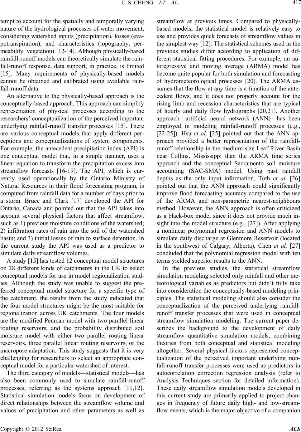

C. S. CHENG ET AL.
417
tempt to account for the spatially an d temporally varying
nature of the hydrological processes of water movement,
considering watershed inpu ts (precipitation), losses (ev a-
potranspiration), and characteristics (topography, per-
meability, vegetation) [12-14]. Although physically-based
rainfall-runoff models can theoretically si mulate the rain-
fall-runoff response, data support, in practice, is limited
[15]. Many requirements of physically-based models
cannot be obtained and calibrated using available rain-
fall-runoff data.
An alternative to the physically-based approach is the
conceptually-based approach. This approach can simplify
representation of physical processes according to the
researchers’ conceptualization of the perceived important
underlying rainfall-runoff transfer processes [15]. There
are various conceptual models that apply different per-
ceptions and conceptualizations of system components.
For example, the antecedent precipitation index (API) is
one conceptual model that, in a simple manner, uses a
linear equation to transform the precipitation excess into
streamflow forecasts [16-19]. The API, which is cur-
rently used operationally by the Ontario Ministry of
Natural Resources in their flood forecasting program, is
computed from rainfall data for a number of days prior to
a storm. Bruce and Clark [17] developed the API for
Ontario, Canada and pointed out that the API takes into
account several physical factors that affect streamflow,
such as 1) previous moisture cond itio ns of the watershe d;
2) infiltration rates of rain into the soil of the watershed
basin; and 3) initial losses of rain to surface detention. In
the current study the API was used as a predictor to
simulate daily streamflow volumes.
A study [15] has tested 12 conceptual model structures
on 28 different kinds of catchments in the UK to select
conceptual models for use in model regionalization stud-
ies. Although the study was unable to suggest the pre-
ferred conceptual model structure for a specific type of
the catchment, the results from the study indicated that
the four model structures might be the most suitable for
regionalization across UK catchments. The four models
are the modified Penman model with two parallel linear
routing reservoirs, and the probability distributed soil
moisture model with either two parallel routing linear
reservoirs, three parallel linear routing reservoirs, or the
macropore adaptation. This study suggests that it is very
challenging for researchers to select an appropriate con-
ceptual model for a particular watershed of interest.
The third category of models—statistical models—has
also been commonly used to simulate rainfall-runoff
processes, referring as the systems approach [11,12].
Statistical simulation models focus on development of
direct relationships between the streamflow volume and
values of precipitation and other parameters as well as
streamflow at previous times. Compared to physically-
based models, the statistical model is relatively easy to
use and provides quick forecasts of streamflow values in
the simplest way [12]. The statistical schemes us ed in the
previous studies differ according to application of dif-
ferent statistical fitting procedures. For example, an au-
toregressive and moving average (ARMA) model has
become quite popular for both simulation and forecasting
of hydrometeorological processes [20]. The ARMA as-
sumes that the flow at any time is a function of the an te-
cedent flows, and it does not properly account for the
rising limb and recession characteristics that are typical
of hourly and daily flow hydrographs [20,21]. Another
approach—artificial neural network (ANN)—has been
employed in modeling rainfall-runoff processes (e.g.,
[22-25]). Hsu et al. [25] pointed out that the ANN ap-
proach provided a better representation of the rainfall-
runoff relationship in the medium-size Leaf River Basin
near Collins, Mississippi than the ARMA time series
approach and the conceptual Sacramento soil moisture
accounting (SAC-SMA) model. Using past rainfall
depths as the only input information, Toth et al. [26]
pointed out that the ANN approach could significantly
improve flood forecasting accuracy compared to the use
of the ARMA and non-parametric nearest-neighbours
method. However, the ANN approach is often criticized
as a black-box model since it does not provide much in-
sight into the model structure (e.g., [27]). After applying
a nonlinear polynomial regression and ANN models to
simulate daily discharge at Glenmore Reservoir (located
in the southwest of Calgary, Alberta), Chen et al. [27]
concluded that the polynomial regression model with ten
terms yielded superior results to the ANN.
In the previous studies, the statistical streamflow
simulation modeling selected only rainfall and other me-
teorological variables as predictors but didn’t fully take
into consideration the co nceptually-based modeling prin-
ciples. The statistical modeling should also consider the
conceptualization of the perceived underlying rainfall-
runoff transfer processes that were used in conceptual
streamflow simulation modeling. The current paper de-
scribes the background to the development of daily
streamflow quantitative simulation models, combining
theories from both conceptual and statistical modeling
altogether. Several physical factors represented concep-
tualization of the perceived important underlying rain-
fall-runoff transfer processes were used as predictors in
autocorrelation correction regression analysis (refer to
Analysis Techniques section for detailed information).
These daily streamflow simulation models developed in
this current study are primarily applied to project chan-
ges in frequency of future daily high- and low-stream-
flow events, which is the major objective of a companion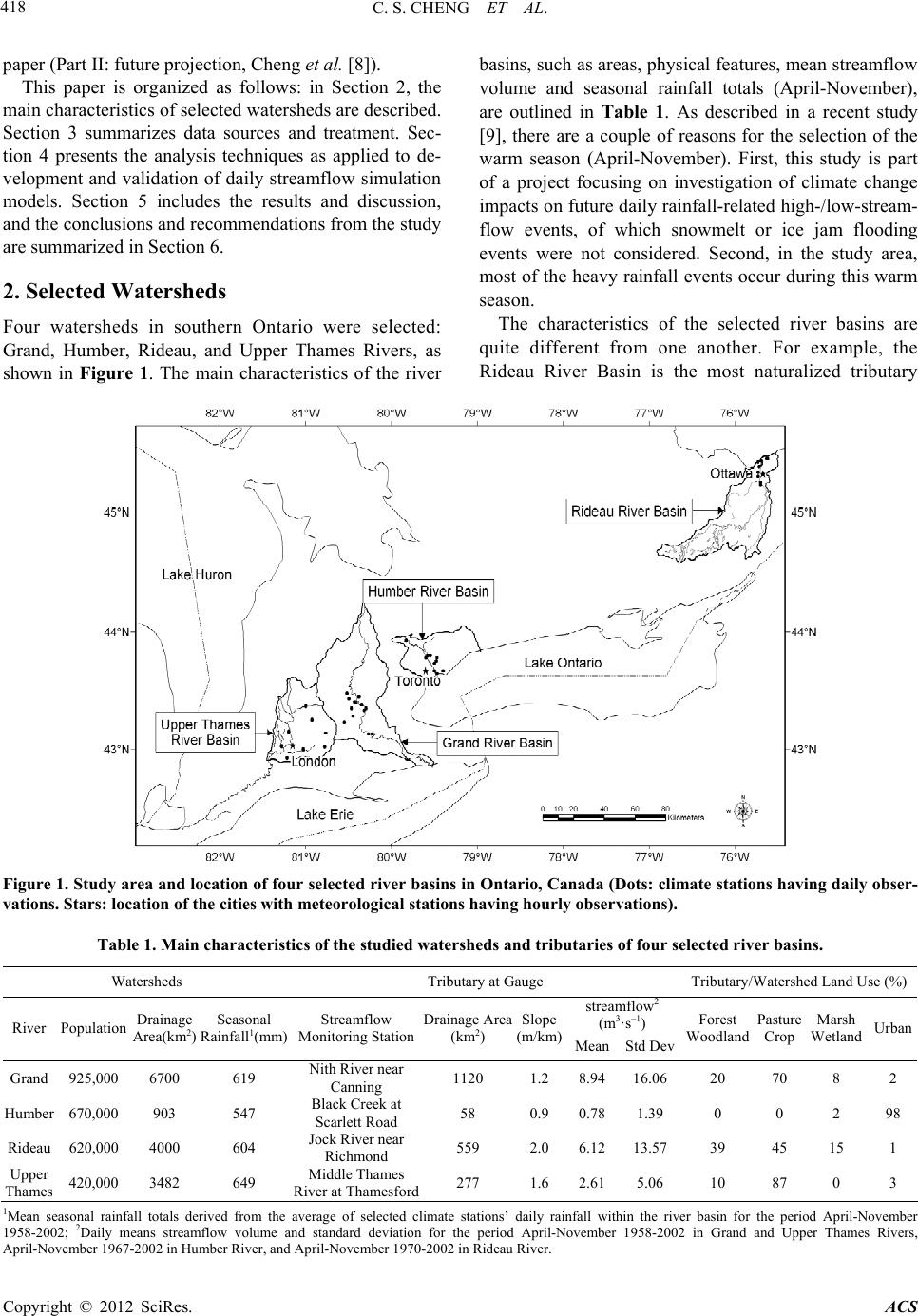

C. S. CHENG ET AL.
418
paper (Part II: fut ure p ro jection , C heng et al. [8]). basins, such as areas, physical features, mean streamflow
volume and seasonal rainfall totals (April-November),
are outlined in Table 1. As described in a recent study
[9], there are a couple of reasons for the selection of the
warm season (April-November). First, this study is part
of a project focusing on investigation of climate change
impacts on future daily rainfall-related high-/low-stream-
flow events, of which snowmelt or ice jam flooding
events were not considered. Second, in the study area,
most of the heavy rainfall events occur during this warm
season.
This paper is organized as follows: in Section 2, the
main characteristics of selected watersheds are described.
Section 3 summarizes data sources and treatment. Sec-
tion 4 presents the analysis techniques as applied to de-
velopment and validation of daily streamflow simulation
models. Section 5 includes the results and discussion,
and the conclusions and recommendations from the study
are summarized in Section 6.
2. Selected Watersheds
The characteristics of the selected river basins are
quite different from one another. For example, the
Rideau River Basin is the most naturalized tributary
Four watersheds in southern Ontario were selected:
Grand, Humber, Rideau, and Upper Thames Rivers, as
shown in Figure 1. The main characteristics of the river
Figure 1. Study area and location of four selected river basins in Ontario, Canada (Dots: climate stations having daily obser-
vations. Stars: location of the cities with meteorological stations having hourly observations).
Table 1. Main characteristics of the studied watersheds and tributaries of four selected river basins.
Watersheds Tributary at Gauge Tributary/Watershed Land Use (%)
streamflow2
(m3·s–1)
River Population
Drainage
Area(km2) Seasonal Rainfall1(mm) Streamflow Monitoring StationDrainage Area (km2) Slope (m/km) MeanStd Dev
Forest
Woodland Pasture Crop Marsh Wetland Urban
Grand 925,000 6700 619 Nith River near
Canning 1120 1.2 8.9416.06 20 70 8 2
Humber 670,000 903 547 Black Creek at
Scarlett Road 58 0.9 0.781.39 0 0 2 98
Rideau 620,000 4000 604 Jock River near
Richmond 559 2.0 6.1213.5739 45 15 1
Upper
Thames 420,000 3482 649 Middle Thames River at Thamesford277 1.6 2.615.06 10 87 0 3
1Mean seasonal rainfall totals derived from the average of selected climate stations’ daily rainfall within the river basin for the period April-November
1958-2002; 2Daily means streamflow volume and standard deviation for the period April-November 1958-2002 in Grand and Upper Thames Rivers,
April-November 1967-2002 in Humber River, and April-November 1970-2002 in Rideau R i ver.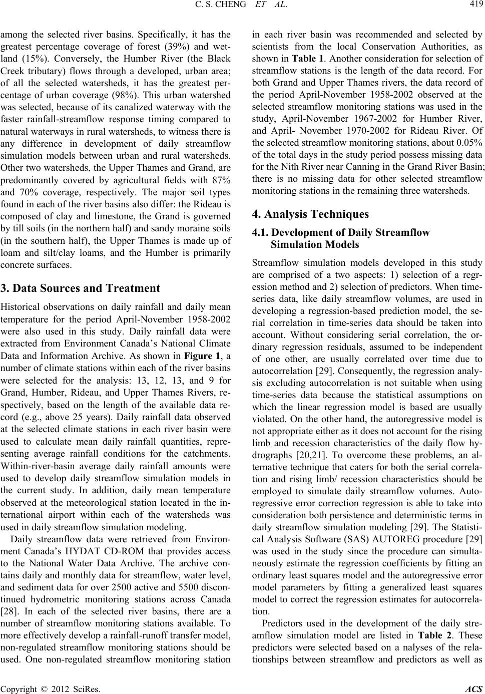

C. S. CHENG ET AL.
419
among the selected river basins. Specifically, it has the
greatest percentage coverage of forest (39%) and wet-
land (15%). Conversely, the Humber River (the Black
Creek tributary) flows through a developed, urban area;
of all the selected watersheds, it has the greatest per-
centage of urban coverage (98%). This urban watershed
was selected, because of its canalized waterway with the
faster rainfall-streamflow response timing compared to
natural waterways in rural watersheds, to witness there is
any difference in development of daily streamflow
simulation models between urban and rural watersheds.
Other two watersheds, the Upper Thames and Grand, are
predominantly covered by agricultural fields with 87%
and 70% coverage, respectively. The major soil types
found in each of the river basins also differ: the Rideau is
composed of clay and limestone, the Grand is governed
by till soils (in the northern half) and sandy moraine soils
(in the southern half), the Upper Thames is made up of
loam and silt/clay loams, and the Humber is primarily
concrete surfaces.
3. Data Sources and Treatment
Historical observations on daily rainfall and daily mean
temperature for the period April-November 1958-2002
were also used in this study. Daily rainfall data were
extracted from Environment Canada’s National Climate
Data and Information Archive. As shown in Figure 1, a
number of climate stations within each of the river basins
were selected for the analysis: 13, 12, 13, and 9 for
Grand, Humber, Rideau, and Upper Thames Rivers, re-
spectively, based on the length of the available data re-
cord (e.g., above 25 years). Daily rainfall data observed
at the selected climate stations in each river basin were
used to calculate mean daily rainfall quantities, repre-
senting average rainfall conditions for the catchments.
Within-river-basin average daily rainfall amounts were
used to develop daily streamflow simulation models in
the current study. In addition, daily mean temperature
observed at the meteorological station located in the in-
ternational airport within each of the watersheds was
used in daily streamflow simulation modeling.
Daily streamflow data were retrieved from Environ-
ment Canada’s HYDAT CD-ROM that provides access
to the National Water Data Archive. The archive con-
tains daily and monthly data for streamflow, water level,
and sediment data for over 2500 active and 5500 discon-
tinued hydrometric monitoring stations across Canada
[28]. In each of the selected river basins, there are a
number of streamflow monitoring stations available. To
more effectively develop a rainfall-runoff transfer model,
non-regulated streamflow monitoring stations should be
used. One non-regulated streamflow monitoring station
in each river basin was recommended and selected by
scientists from the local Conservation Authorities, as
shown in Table 1. Another consideration for selection of
streamflow stations is the length of the data record. For
both Grand and Upper Thames rivers, the data record of
the period April-November 1958-2002 observed at the
selected streamflow monitoring stations was used in the
study, April-November 1967-2002 for Humber River,
and April- November 1970-2002 for Rideau River. Of
the selected streamflow monitoring stations, about 0.05%
of the total days in the stud y period possess missing data
for the Nith River near Canning in the Grand River Basin;
there is no missing data for other selected streamflow
monitoring stations in the remaining three watersheds.
4. Analysis Techniques
4.1. Development of Daily Streamflow
Simulation Models
Streamflow simulation models developed in this study
are comprised of a two aspects: 1) selection of a regr-
ession method and 2) selection of predictors. When time-
series data, like daily streamflow volumes, are used in
developing a regression-based prediction model, the se-
rial correlation in time-series data should be taken into
account. Without considering serial correlation, the or-
dinary regression residuals, assumed to be independent
of one other, are usually correlated over time due to
autocorrelation [ 29]. Consequently, the regression analy-
sis excluding autocorrelation is not suitable when using
time-series data because the statistical assumptions on
which the linear regression model is based are usually
violated. On the other hand, the autoregressive model is
not appropriate either as it does not account for the rising
limb and recession characteristics of the daily flow hy-
drographs [20,21]. To overcome these problems, an al-
ternative technique that caters for both the serial correla-
tion and rising limb/ recession characteristics should be
employed to simulate daily streamflow volumes. Auto-
regressive error correction regression is able to take into
consideration both persistence and deterministic terms in
daily streamflow simulation modeling [29]. The Statisti-
cal Analysis Software (SAS) AUTOREG procedure [29]
was used in the study since the procedure can simulta-
neously estimate the regression coefficients by fitting an
ordinary least squares model and the autoregressive error
model parameters by fitting a generalized least squares
model to correct the regression estimates for autocorrela-
tion.
Predictors used in the development of the daily stre-
amflow simulation model are listed in Table 2. These
predictors were selected based on a nalyses of the rela-
tionships between streamflow and predictors as well as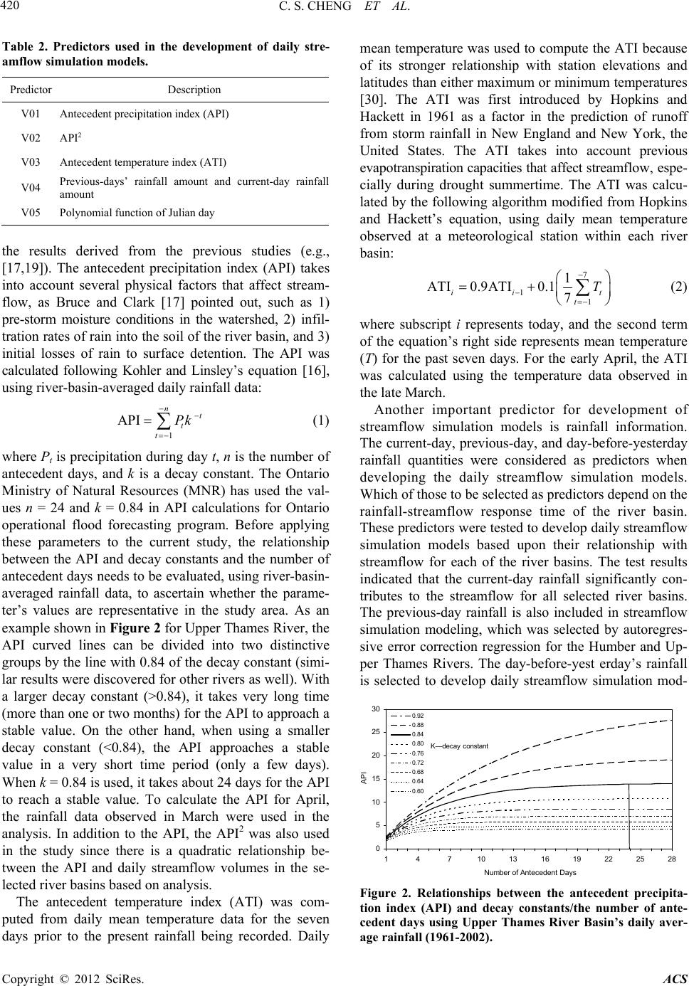

C. S. CHENG ET AL.
420
Table 2. Predictors used in the development of daily stre-
amflow simulation models.
Predictor Description
V01 Antecedent precipitation index (API)
V02 API2
V03 Antecedent tem perature index (ATI)
V04 Previous-days’ rainfall amount and current-day rainfall
amount
V05 Polynomial function of Julian day
the results derived from the previous studies (e.g.,
[17,19]). The antecedent precipitation index (API) takes
into account several physical factors that affect stream-
flow, as Bruce and Clark [17] pointed out, such as 1)
pre-storm moisture conditions in the watershed, 2) infil-
tration rates of rain into the soil of the river basin, and 3)
initial losses of rain to surface detention. The API was
calculated following Kohler and Linsley’s equation [16],
using river-basin-averaged daily rainfall data:
1
Int
t
t
Pk


 AP (1)
where Pt is precipitation during da y t, n is the number of
antecedent days, and k is a decay constant. The Ontario
Ministry of Natural Resources (MNR) has used the val-
ues n = 24 and k = 0.84 in API calculations for Ontario
operational flood forecasting program. Before applying
these parameters to the current study, the relationship
between the API and decay constants and the number of
antecedent days needs to be evaluated, using river-basin-
averaged rainfall data, to ascertain whether the parame-
ter’s values are representative in the study area. As an
example shown in Figure 2 for Upper Thames River, the
API curved lines can be divided into two distinctive
groups by the line with 0.84 of the decay constant (simi-
lar results were discovered for other rivers as well). With
a larger decay constant (>0.84), it takes very long time
(more than one or two months) for the API to approach a
stable value. On the other hand, when using a smaller
decay constant (<0.84), the API approaches a stable
value in a very short time period (only a few days).
When k = 0.84 is used, it takes about 24 days for the API
to reach a stable value. To calculate the API for April,
the rainfall data observed in March were used in the
analysis. In addition to the API, the API2 was also used
in the study since there is a quadratic relationship be-
tween the API and daily streamflow volumes in the se-
lected river basins based on analysis.
The antecedent temperature index (ATI) was com-
puted from daily mean temperature data for the seven
days prior to the present rainfall being recorded. Daily
mean temperature was used to compute the ATI because
of its stronger relationship with station elevations and
latitudes than eith er maximum or minimum temperatures
[30]. The ATI was first introduced by Hopkins and
Hackett in 1961 as a factor in the prediction of runoff
from storm rainfall in New England and New York, the
United States. The ATI takes into account previous
evapotranspiration capacities that affect streamflow , esp e-
cially during drought summertime. The ATI was calcu-
lated by the following algorithm modified from Hopkins
and Hackett’s equation, using daily mean temperature
observed at a meteorological station within each river
basin:
7
11
1
ATI0.9ATI0.1 7
ii t
t
T







 (2)
where subscript i represents today, and the second term
of the equation’s right side represents mean temperature
(T) for the past seven days. For the early April, the ATI
was calculated using the temperature data observed in
the late March.
Another important predictor for development of
streamflow simulation models is rainfall information.
The current-day, previous-day, and day-before-yesterday
rainfall quantities were considered as predictors when
developing the daily streamflow simulation models.
Which of those to be selected as predictors depend on the
rainfall-streamflow response time of the river basin.
These predictors were tested to develop daily streamflow
simulation models based upon their relationship with
streamflow for each of the river basins. The test results
indicated that the current-day rainfall significantly con-
tributes to the streamflow for all selected river basins.
The previous-day rainfall is also included in streamflow
simulation modeling, which was selected by autoregres-
sive error correction regression for the Humber and Up-
per Thames Rivers. The day-before-yest erday’s rainfall
is selected to develop daily streamflow simulation mod-
0
5
10
15
20
25
30
147 10131619222528
API
0.92
0.88
0.84
0.80
0.76
0.72
0.68
0.64
0.60
K—decay constant
Number of Antecedent Days
Figure 2. Relationships between the antecedent precipita-
tion index (API) and decay constants/the number of ante-
cedent days using Upper Thames River Basin’s daily aver-
age rainfall (1961-2002).

C. S. CHENG ET AL.
421
els for the Grand and Rideau Rivers.
The last predictor used in th e daily streamflow simula-
tion modeling represents streamflow seasonal variation.
Streamflow volumes possess a seasonal variation: high
flow usually occurs in the spring as a result of the melt-
ing of accumulated winter snowfall; summer and autumn
are the seasons of generally low flows as a result of the
depletion of groundwater reservoirs during these months
(Figure 3). Such seasonal variation should be taken into
account when developing daily streamflow simulation
models. As shown in Figure 3, a fourth-order polyno-
mial function of Julian day best fits the daily mean
streamflow data for the four selected river basins, with
model R2s of 0.87, 0.88, and 0.91 for the Upper Thames,
Grand, and Rideau rivers, respectively. However, the
model R2 of 0.33 for Humber River is much lower than
other river basins. The possible reason for this might be
that the daily streamflow volume in Humber River Basin
is much lower than it is in three other river basins; con-
sequently, the seasonal variation is much smaller. Al-
though the polynomial function of Julian day is devel-
oped from year-round recorded data, only eight months
(April– November) of the time are actually used in the
daily streamflow simulation modeling.
4.2. Validation of Daily Streamflow Simulation
Models
The daily streamflow simulation models were validated
using a leave-one-year-out cross-validation procedure, in
which the regression procedure was repeatedly run to
develop a streamflow simulation model that would vali-
date one year of independent data for each year in the
dataset. The validated data were then compared with
observations to evaluate model performance. As a result,
the number of simulation models developed in the study
is the number of the total years used in the analysis. For
example, in the Upper Thames River Basin the data ob-
served for the period 1958-2002 were used in the devel-
opment and validation of daily streamflow simulation
models; therefore, 45 models in total were developed.
Each model was developed using 44 years of data and
one-year data were withheld to validate the model. One
of the advantages using the cross-validation procedure is
that it is able to use a series of models to evaluate the
reliability of the streamflow simulation models when the
models’ performances are consistent at a certain level.
5. Results and Discussions
Daily streamflow simulation models developed by auto-
regressive error correction regression for all selected
river basins, of which one model for each river basin is
shown in Table 3 as an example. This model was devel-
oped when the data for the year 1979 were withheld as an
independent dataset for validation of the model. As
shown in Table 3, there are significant correlations be-
tween daily streamflow volumes and model simulations,
with model R2s of 0.62, 0.71, 0.74, and 0.95 for Humber,
Grand, Upper T hames, and Rideau River basins, re-
Grand River: Nith River near Canning
y = 38.395-0. 956* x+ 8. 8 6E -3*x2-3.27E-5*x3+4.249E-8*x4
R2 = 0.88 RMS E = 3. 00
0
5
10
15
20
25
30
35
40
45
AMJJ ASONDJ FM
Daily Mean Streamflow (m
3
/s)
Rideau River: Jock River near Richmond
y = 42.29 8-1.108*x +9. 92E-3*x 2-3.56E-5*x3+4.474E-08*x4
R2 = 0. 91 RM S E = 2.49
-5
0
5
10
15
20
25
30
35
40
45
AMJJASONDJFM
y = 11.08 5-0.262*x +2. 33E-3*x 2-8.33E-6*x3+1.079E-8*x4
R2 = 0. 87 RM S E = 1. 02
0
2
4
6
8
10
12
14
AM J JASOND JFM
Month
Upper Thames River: Middle Thames River at Thamesford
Humber River: Black C reek at Sc arlet t R oad
y = 1.30 7-0.0177*x +1. 73E-4*x 2-6.915E-7*x3+9.592E-10*x4
R2 = 0. 33 RM S E = 0. 24
0.0
0.5
1.0
1.5
2.0
2.5
3.0
3.5
4.0
4.5
5.0
AMJ J ASONDJ FM
Month
Daily Mean Streamflow (m
3
/s)
Figure 3. Polynomial function of Julian Day fitting daily mean streamflow volumes for the selected streamflow stations.

C. S. CHENG ET AL.
422
Table 3. Summary of the streamflow simulation models
when the data of the year 1979 withheld as an independent
dataset for validation of the model in the four selected river
basins.
Variable EstimateStd Err t Value Approx Pr > |t|
Grand River Basin (R2 = 0.71, RMSE = 7.50)
Intercept –4.44270.9743 –4.56 <0.0001
API 0.5021 0.0454 11.07 <0.0001
API2 0.0002 0.0009 0.18 0.8578
ATI –0.24540.0471 –5.21 <0.0001
Julian Day 0.9752 0.0556 17.53 <0.0001
Current-Day Rainfall 0.0035 0.0169 0.21 0.8372
Day-before-Yesterday
Rainfall 0.5275 0.0145 36.39 <0.0001
AR1 –0.75440.0054 –139.18 <0.0001
Humber River Basin (R2 = 0.62, RMSE = 0.75)
Intercept –0.29990.0557 –5.38 <0.0001
API 0.0151 0.0028 5.43 <0.0001
API2 0.000020.0001 0.31 0.7576
ATI –0.02550.0012 –21.71 <0.0001
Julian Day 0.7610 0.0619 12.30 <0.0001
Current-Day Rainfall 0.1313 0.0018 73.66 <0.0001
Previous-Day Rainfal l 0.1573 0.0022 72.68 <0.0001
AR1 –0.11000.0089 –12.37 <0.0001
Rideau River Basin (R2 = 0.95, RMSE = 2.95 )
Intercept 4.3389 0.9030 4.81 <0.0001
API 0.1983 0.0165 12.02 <0.0001
API2 0.0015 0.0003 5.06 <0.0001
ATI –0.25230.0586 –4.31 <0.0001
Julian Day 0.1612 0.0258 6.24 <0.0001
Current-Day Rainfall 0.0226 0.0059 3.83 0.0001
Day-before-Yesterday
Rainfall 0.0608 0.0046 13.13 <0.0001
AR1 –0.96260.0025 –375.75 <0.0001
Upper Thames River Basin (R2 = 0.74, RMSE = 2.40)
Intercept –2.32470.3478 –6.68 <0.0001
API 0.2190 0.0160 13.66 <0.0001
API2 0.0040 0.0003 13.08 <0.0001
ATI –0.14520.0174 –8.36 <0.0001
Julian Day 0.9333 0.0593 15.74 <0.0001
Current-Day Rainfall 0.0406 0.0059 6.89 <0.0001
Previous-Day Rainfal l 0.0546 0.0070 7.76 <0.0001
AR1 –0.73120.0056 –130.55 <0.0001
Note: RMSE = root mean squared error; API = antecedent precipitation
index; ATI = antecedent temperature index; AR1 = the order 1 or lag 1
autocorr elation paramet er; Estimate = the coeff icient of t he regressi on algo-
rithm; and Std Err = standard error.
spectively. The simulation models have identified that
the predictors are consistent with the physical processes
typically associated with high flow events. From the
simulation models provided in Table 3 it is seen that the
first-order autoregressive process (AR1), which repre-
sents the serial correlation of streamflow itself and the
explanatory predicto rs, sign ificantly contribute to stream-
flow simulation. Since a negative AR1 is built in the
autoregressive error correction modeling, there is a posi-
tive relationship between the AR1 and daily streamflow
volumes. In addition to the persistence of high-stream-
flow, rainfall/moisture conditions (i.e., today/previous-
day rainfall and API) and streamflow seasonal variation
(i.e., polynomial function of Julian day) are positively
associated with daily streamflow volumes. Furthermore,
there is a significantly negative relationship between the
ATI and daily streamflow volumes since the ATI repre-
sents evapotranspiration within the river basins. The ro-
bustness of the developed streamflow simulation models
is examined considering not only the AR1 but also the
higher order parameters, such as the second-order to
fifth-order autoregressive processes. The test results
showed that considering any of higher order parameters,
the simulation models didn’t improve much on the model
performance in terms of model R2 (with 0.00 - 0.02 in-
crease) and root mean squared errors (with 0.0 - 0.2
m3·s–1 decrease). As a result, it is not necessary to con-
sider any of order parameters higher than the first-order
autoregressive process in the daily streamflow simulation
modeling.
In addition to sample models summarized in Table 3,
all streamflow simulation models’ R2s and root mean
squared errors (RMSEs) for the selected river basins are
shown in Table 4. For reference, overall daily mean
streamflow volume and standard deviation for the entire
study period are also listed in Table 4. Furthermore, the
comparison between streamflow observations and model
validations is illustrated in Figure 4, of which the model
R2s and RMSEs are very similar to the model simulations
as shown in Table 4. To effectively measure difference
between model simulations and validations, the differ-
ence between the two data sample means and variances
was analyzed, respectively using t- and F-tests; no sig-
nificant (<0.05 level) difference between the daily
streamflow simulations and validations was detected. It
implies that the stream- flow simulation models devel-
oped in the study are reliable with a great potential to be
used to downscale future daily streamflow volumes at a
local scale.
From Table 4 and Figure 4, it can be seen that the
streamflow simulation model performance for Upper Th-
ames and Grand Rivers is very similar, with model R2s
ranging from 0.68 to 0.74. The streamflow simulation

C. S. CHENG ET AL. 423
models for Rideau River demonstrated the strongest
models of the selected river basins with R2 of 0.95; for
Humber River, the simulation models are the weakest
with R2 ranging from 0.61 to 0.62. This implies that the
methods used in the study are more suitable to develop
simulation models of daily rainfall- related streamflow
volumes for nature waterways in rural watersheds, such
as Rideau, Grand, and Upper Thames Rivers. The meth-
ods are limited for an urban river basin like the Black
Creek tributary of the Humber River. The reasons for this
might be that rainfall-streamflow hydrological response
time and physical characteristics differ significantly be-
tween urban and rural river basins as described as fol-
lows:
1) The API is not a good indicator to simulate daily
streamflow for an urban river basin like the Humber
River. As discussed above, the API takes into account
several physical factors that affect streamflow, including
previous soil moisture conditions of the watershed. The
API is suitable to characterize the soil moisture condi-
tions for rural river basins (e.g., Grand, Rideau, and Up-
per Thames) but not for urban river basins with a con-
crete waterway (e.g., Humber River).
2) The serial correlation of daily streamflow volumes,
presented by the AR1 in streamflow simulation models,
varies among the river basins. From Table 3, the AR1s
for Rideau and Humber Rivers are the largest (–0.96) and
smallest (–0.11) of the selected river basins, respectively;
the parameters for Grand and Upper Thames Rivers fall
in the middle with the similar values (i.e. , –0.77 and
–0.73).
3) The seasonal variation of daily mean streamflow
(the polynomial function of Ju l i a n day) , whi ch is another
Table 4. Streamflow simulation model R2s and root mean
squared errors (RMSE), using a leave-one-year-out cross-
validation scheme, for the selected river basins (overall
daily mean streamflow volume and standard deviation are
listed for reference).
River Basin Grand Humber Rideau Upper Thames
Model R2 0.68 - 0.710.61 - 0.62 0.95 - 0.95 0.71 - 0.74
RMSE (m3·s–1)7.71 - 8.030.74 - 0.76 2.85 - 2.95 2.40 - 2.56
Daily mean
(Std Dev) (m3·s–1)8.94 (16.06)0.78 (1.39) 6.12 (13.57) 2.61 (5.06)
Note: Overall daily mean streamflow volume and standard deviation were
calculated for the period April-November 1958-2002 in Grand and Upper
Thames Rivers, April-November 1967-2002 in Humber River, and April-
November 1970-2002 in Rideau Rive r.
Gr and River Basin
R
2
= 0.70
RMSE = 8.72
0
40
80
120
160
200
240
280
320
04080120 160200 240280 320
Verifica tion (m
3
s
-1
)
Ri deau River Basin
R
2
= 0.95
RMSE = 2.98
0
15
30
45
60
75
90
105
120
135
150
0153045607590105120 135150
Humber River Basin
R
2
= 0.61
RMSE = 0.87
0
5
10
15
20
25
0510 1520 25
O bservation
(
m
3
s
-1
)
Upper Thames River Basi n
R
2
= 0. 73
RMSE = 2.61
0
15
30
45
60
75
90
105
120
0 15304560759010512
Verification (m
3
s
-1
)
0
Obser vati on (m
3
s
-1
)
Figure 4. Relationships between streamflow observations and model validations using a leave-one-year-out cross-validation
scheme in the selected river basins (solid line represents a regression line; dashed line is a perfect fit. Grand and Upper
Thames Rivers: 1958-2002; Humber River: 1967-2002; Rideau River: 1970-2002).

C. S. CHENG ET AL.
424
important predictor to simulate daily streamflow volumes,
differs between the river basins. The stronger the sea-
sonal variation is, the more the predictor contributes to
streamflow simulation. As shown in Figure 3, the model
R2 of a fourth-order polynomial function of Julian day is
0.91 for Rideau River and 0.33 for Humber River, which
is the largest and smallest model R2 of the selected river
basins. The model R2s for Grand and Upper Thames
Rivers are 0.88 and 0.87 , resp ect i vely .
4) An additional possible reason for the weakest daily
streamflow simulation model in the Humber River Basin
might be that the daily streamflow volume observed at
the station Black Creek near Scarlett Road of Humber
River is usually quite small. From Table 1 it is seen that
overall daily mean streamflow volume during the entire
study time period in the Grand, Rideau, and Upper
Thames Rivers is 11.5, 7.8, and 3.3 times as high as that
in the Humber River. The statistical methods used in the
study could be restricted when the daily streamflow vol-
ume is very low.
5) The last possible reason for the weakest daily
streamflow simulation model in the Humber River Basin
might be limitation of streamflow data. The streamflow
data used in the study are daily mean flows which are
averaged over a 24-hour period (i.e., 00:00-23:00 LST),
and are currently available from the Environment Can-
ada’s National Water Data Archive. For rapidly rainfall-
streamflow responding urban watersheds (e.g., the Black
Creek tributary of the Humber River), daily mean stream-
flow data are limited in their usefulness for studying
more detailed information on the simulation of the high-
streamflow events. If the short-duration (less than one
day) streamflow data were available, the streamflow sim-
ulation models for the Humber River Basin could possi-
bly be improved by using streamflow information at a
shorter time step.
6. Conclusions and Recommendation
The purpose of this study was to collectively apply both
conceptual and statistical modeling theories to develop
daily streamflow simulation models for four selected
river basins in the Province of Ontario, Canada. The
simulation models demonstrated significant skill in the
discrimination and prediction of daily streamflow vol-
umes as well as occurrence of high-/low-streamflow
events. A formal model result verification process has
been built into the exercise, using a leave-one-year-out
cross scheme. The results have shown that there are sig-
nificant correlations between daily streamflow observa-
tions and model validations, with model R2s of 0.68 -
0.71, 0.61 - 0.62, 0.71 - 0.74, and 0.95 for Grand, Hum-
ber, Upper Thames, and Rideau River Basins, respec-
tively. As a result, a general con clusion from this stud y is
that the methods used in the analysis are suitable to be
used for projection or downscaling of changes in fre-
quency of future daily high-/low-streamflow events at a
local scale, which is the major objective of a companion
paper (Part II: future projection, Cheng et al. [8]). To
achieve this, the research work should include the fol-
lowing three aspects. First, the downscaled future daily
rainfall data at a river-basin local scale are required,
which have been derived by Cheng et al. [9,10]. Second,
the statistical downscaling method developed by Cheng
et al. [31] will be adapted to downscale future GCM
simulations to the selected meteorological stations for
weather variables that were used in the daily streamflow
simulation modeling. Third, future daily streamflow
volumes can be projected by applying daily streamflow
simulation models developed in the current study with
downscaled future climate information.
In this study, the streamflow simulation models are
river-basin-specific since the predictors were selected
and constructed based on characteristics/relationships
specific to the selected river basins. Therefore, to apply
these models at other locations, they have to be recreated
each time using locally measured data. The methods of
streamflow simulation modeling, including predictor
selection/construction processing, can be adopted to any
other river basin influenced by a variety of topographic
and other factors to build a new streamflow simulation
model.
7. Acknowledgements
The authors gratefully acknowledge the funding support
of the Government of Canada’s Climate Change Impacts
and Adaptation Program (CCIAP), which made this re-
search project (A901) possible. We also acknowledge the
suggestions made by the Project Advisory Committee,
which greatly improved the study.
REFERENCES
[1] D. Panagoulia and G. Dimou, “Sensitivity of Flood
Events to Global Climate Change,” Journal of Hydrology,
Vol. 191, No. 1-4, 1997, pp. 208-222.
doi:10.1016/S0022-1694(96)03056-9
[2] R. G. Najjar, “The Water Balance of the Susquehanna
River Basin and Its Response to Climate Change,” Jour-
nal of Hydrology, Vol. 219, No. 1-2, 1999, pp. 7-19.
doi:10.1016/S0022-1694(99)00041-4
[3] G. Drogue, L. Pfister, T. Leviandier, A. El Idrissi, J-F.
Iffly, P. Matgen, J. Humbert and L. Hoffmann, “Simulat-
ing the Spatio-Temporal Variability of Streamflow Re-
sponse to Climate Change Scenarios In a Mesoscale Ba-
sin,” Journal of Hydrology, Vol. 293, No. 1-4, 2004, pp.
255-269.
[4] D. Nohara, A. Kitoh, M. Hosaka and T. Oki, “Impact of

C. S. CHENG ET AL. 425
Climate Change on River Discharge Projected by Multi-
model Ensemble,” Journal of Hydrometeorology, Vol. 7,
No. 5, 2006, pp. 1076-1089. doi:10.1175/JHM531.1
[5] A. L. Kay, R. G. Jones and N. S. Reynard, “RCM Rain-
fall for UK Flood Frequency Estimation. II: Climate
Change Results,” Journal of Hydrology, Vol. 318, No. 1-4,
2006, pp. 163-172.
doi:10.1016/j.jhydrol.2005.06.013
[6] W. S. Merritt, Y. Alisa, M. Barton, B. Taylor, S. Cohen
and D. Neilsen, “Hydrologic Response to Scenarios of
Climate Change in Sub-Watersheds of the Okanagan Ba-
sin, British Columbia,” Journal of Hydrology, Vol. 326,
No. 1-4, 2006, pp. 79-108.
doi:10.1016/j.jhydrol.2005.10.025
[7] Public Safety and Emergency Preparedness, “Canadian
Disaster Database Version 4.4,” Canada, 2006.
[8] C. S. Cheng, Q. Li, G. Li and H. Auld, “Possible Impacts
of Climate Change on Future Daily Streamflow and Ex-
tremes at Local Scale in Ontario, Canada. Part II: Future
projection,” Atmospheric and Climate Sciences, Vol. 2,
No. 4, 2012, pp. 427-440.
[9] C. S. Cheng, G. Li, Q. Li and H. Auld, “A Synoptic Wea-
ther Typing Approach to Simulate Daily Rainfall and Ex-
tremes in Ontario, Canada: Potential for Climate Change
Projections,” Journal of Applied Meteorology and Cli-
matology, Vol. 49, No. 5, 2010, pp. 845-866.
doi:10.1175/2010JAMC2016.1
[10] C. S. Cheng, G. Li, Q. Li and H. Auld, “A Synoptic
Weather-Typing Approach to Project Future Daily Rain-
fall and Extremes at Local Scale in Ontario, Canada,”
Journal of Climate, Vol. 24, No. 14, 2011, pp. 3667-3685.
doi:10.1175/2011JCLI3764.1
[11] E. F. Wood and P. E. O’Connell, “Real-Time Forecast-
ing,” In: M. G. Anderson and T. B. Burt, Eds., Hydrology
Forecasting, John Wiley & Sons Ltd., New York, 1985,
pp. 505-558.
[12] H. Gupta, “Hydrological Modeling for Runoff Forecast-
ing,” In: T. D. Potter and B. Colman, Eds., Handbook of
Weather, Climate, and Water: Atmospheric Chemistry,
Hydrology, and Societal Impacts, John Wiley & Sons,
Inc., Hoboken, 2003, pp. 571-586.
[13] K. Solander, L. Saito and F. Biondi, “Streamflow Simula-
tion Using a Water-Balance Model with Annually-Re-
solved Inputs,” Journal of Hydrology, Vol. 387, No. 1-2,
2010, pp. 46-53. doi:10.1016/j.jhydrol.2010.03.028
[14] C. Yang, Z. Lin, Z. Yu, Z. Hao and S. Liu, “Analysis and
Simulation of Human Activity Impact on Streamflow in
the Huaihe River Basin with a Large-Scale Hydrologic
Model,” Journal of Hydrometeorology, Vol. 11, No. 3,
2010, pp. 810-821. doi:10.1175/2009JHM1145.1
[15] H. Lee, N. McIntyre, H. Wheater and A. Young, “Selec-
tion of Conceptual Models for Regionalisation of the
Rainfall-Runoff Relationship,” Journal of Hydrology, Vol.
312, No. 1-4, 2005, pp. 125-147.
doi:10.1016/j.jhydrol.2005.02.016
[16] M. A. Kohler and R. K. Linsley, Jr., “Predicting Runoff
from Storm Rainfall,” Research Paper 34, US Weather
Bureau, Washington DC, 1951.
[17] M. A. Bruce and R. H. Clark, “Introduction to Hydrome-
teorology,” Pergamon Press, Oxford, 1966.
[18] W. T. Sittner, C. E. Schauss and J. C. Monro, “Continu-
ous Hydrograph Synthesis with an API-Type Hydrologic
Model,” Water Resources Research, Vol. 5, No. 5, 1969,
pp. 1007-1022. doi:10.1029/WR005i005p01007
[19] R. J. Heggen, “Normalized Antecedent Precipitation In-
dex,” Journal of Hydrologic Engineering, Vol. 6, No. 5,
2001, pp. 377-381.
doi:10.1061/(ASCE)1084-0699(2001)6:5(377)
[20] J. D. Salas and R. A. Pielke, “Stochastic Characteristics
and Modeling of Hydroclimatic Processes,” In: T. D. Pot-
ter and B. Colman, Eds., Handbook of Weather, Climate,
and Water: Atmospheric Chemistry, Hydrology, and So-
cietal Impacts, John Wiley & Sons, Inc., Hoboken, 2003,
pp. 587-605.
[21] R. K. Linsley, “Rainfall-Runoff Models—An Overview,”
In: V. P. Singh, Ed., Rainfall-runoff Relationship, Book-
Crafters Inc., Kansas City, 1981, pp 3-22.
[22] K. Hsu, H. V. Gupta and S. Sorooshian, “Artificial Neural
Network Modeling of the Rainfall-Runoff Process,” Wa-
ter Resources Research, Vol. 31, No. 10, 1995, pp. 2517-
2530. doi:10.1029/95WR01955
[23] J. M. Ehrman, K. Higuchi and T. A. Clair, “Backcasting
to Test the Use of Neural Networks for Predicting Runoff
in Ca nadia n Ri vers ,” Canadian Water Resources Journal,
Vol. 25, No. 3, 2000, pp. 279-291.
doi:10.4296/cwrj2503279
[24] A. Nazemi, H. N. Poorkhadem, R. Mohammad, T. Ak-
barzadeh and S. M. Hosseini, “Evolutionary Neural Net-
work Modeling for Describing Rainfall-Runoff Process,”
Hydrology Days, 2003, pp. 224-235.
[25] T. Asefa, “Ensemble Streamflow Forecast: A Glue-Based
Neural Network Approach,” Journal of the American
Water Resource Association, Vol. 45, No. 5, 2009, pp.
1155-1163. doi:10.1111/j.1752-1688.2009.00351.x
[26] E. Toth, A. Brath and A. Montanari, “Comparison of
Short-Term Rainfall Prediction Models for Real-Time
Flood Forecasting,” Journal of Hydrology, Vol. 239, No.
1-4, 2000, pp. 132-147.
doi:10.1016/S0022-1694(00)00344-9
[27] L. Chen, F. J. C. Bouchart and J. W. Davison, “Applica-
tion of a New Polynomial Regression Method Based on
Genetic Programming in Hydrologic Modeling,” The
First Biennial Workshop of the Statistical Hydrology, Cana-
dian Geophysical Union, Calgary, 18-21 May 2002, 6 pp.
[28] Environment Canada, “HYDAT CD-ROM,” 2006.
http://www.wsc.ec.gc.ca/products/hydat/main_e.cfm?cna
me=hydat_e.cfm
[29] SAS Institute Inc., “The AUTOREG Procedure: Regres-
sion with Autocorrelation Errors,” 2006.
http://support.sas.com/91doc/docMainpage.jsp
[30] C. D. Hopkins Jr. and D. O. Hackett, “Average Antece-
dent Temperatures As a Factor in Predicting Runoff from
Storm Rainfall,” Journal of Geophysical Research, Vol.
66, No. 10, 1961, 3313-3318.
doi:10.1029/JZ066i010p03313
[31] C. S. Cheng, G. Li, Q. Li and H. Auld, “Statist ical Down-

C. S. CHENG ET AL.
426
scaling of Hourly and Daily Climate Scenarios for Vari-
ous Meteorological Variables in South-Central Canada,” Theoretical and Applied Climatology, Vol. 91, No. 1-4, 2008, pp. 129-147. doi:10.1007/s00704-007-0302-8
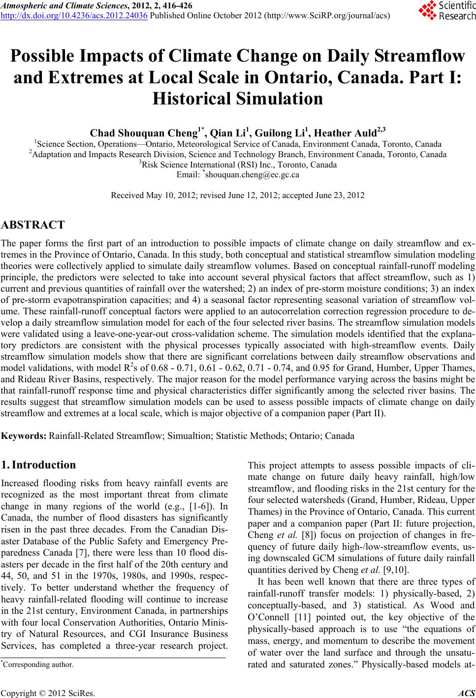