Journal of Geographic Information System, 2012, 4, 479-482
http://dx.doi.org/10.4236/jgis.2012.45052 Published Online October 2012 (http://www.SciRP.org/journal/jgis)
The Thermal Inertia Characteristics of the System
Ocean-Atmosphere
Habibullo I. Abdussamatov, Sergey I. Khankov, Yevgeniy V. Lapovok
Space Research of the Sun Sector, Pulkovo Observatory, St. Petersburg, Russia
Received August 7, 2012; revised September 6, 2012; accepted October 8, 2012
ABSTRACT
To estimate the time delay between the planetary temperature change and the change of the incoming solar radiation
fraction absorbed by the ocean and the atmosphere, the analytical energy balance model is presented. The model gener-
alization allows of using averaged data for model parameterization. Using the model, the time delay is investigated on
four model cases of absorbed radiation change. The interconnections among the time delay, the planetary thermal iner-
tia and the ocean active layer depth are established.
Keywords: Thermal Inertia; Planetary Temperature; Total Solar Irradiance; System Ocean-Atmosphere
1. Introduction
Theoretical studies of the Earth’s temperature change re-
lated to the change of the solar incoming absorbed by the
Earth are based on model development with parameteri-
zation based on empirical data. Main approaches to model
development are general circulation models (GCMs), sta-
tistical dynamical models (SDMs) and energy balance
models (EBMs).
EBMs have been developed extensively after Budyko
[1] and Sellers [2] published their models. Models of this
type are relatively simple in comparison with GSMs and
place more emphasis upon obtaining strong theoretical
and analytical results in comparison with SDMs. Com-
monly for EBM, the model surface temperature is an
unknown function of time obtaining from the one-di-
mensional equation, whereas zonal and seasonal varia-
tions of key climate parameters are taken into account
through empirical data. The paper [3] contains a reex-
amination of EBMs developed before year 1981, and the
papers [4-7] are samples of the results of modern EBM
development.
The important attribute of the models described above
is their attempt to include the zonal and seasonal varia-
tions of the outgoing infrared flux, the incoming solar
flux and the space-dependent heat capacity. This model
presents the energy balance model with two important
features. First, our model is generalized and based on the
specific heat capacity for the ocean and the atmosphere
per unit surface [m2] averaged over the Earth’s surface
and on the annual averaged solar irradiation. Second, the
Earth is considered as a system of the ocean and the at-
mosphere.
This approach makes it possible to research the dy-
namic of the transition of the system ocean-atmosphere
from one quasi-equilibrium state to another for model
cases of the absorbed solar flux change. In addition, this
approach makes it possible to reduce the term “the cli-
mate sensitivity” to the “thermal inertia” determined
mainly by the ocean heat capacity.
Our study is aimed at determination of the time lag τ
between the increment of the global planetary thermo-
dynamic temperature,
 = Tp − Tpo, (here Tp and Tpo are
the planetary temperature and its initial value, respec-
tively) and the increment of the specific power of thermal
emission, Q, in the ocean and the atmosphere, caused
by fluctuations of the total solar irradiance and/or Bond
albedo. Our investigations have been performed for typ-
ical model cases of the temporal changes of the incre-
ment Q which simplifies determination of the factors
decelerating the process of transition into a new thermal
state.
2. Mathematical Modeling
To investigate the planetary thermal inertia and the time
lag, it is necessary to investigate the Earth’s heat tran-
sient state taking into account the absorbed solar irradia-
tion and the outgoing infrared flux.
In the previous paper [8] we obtained the non-steady
equation of the planetary heat balance. Given the incre-
ment of the planetary absorbed solar irradiation and the
related planetary temperature increment
 , the equation
is reconsidered in form
C
opyright © 2012 SciRes. JGIS

H. I. ABDUSSAMATOV ET AL.
480
 
4
d11
d
;;
;
p
po
o
po
t
c
taT
3
;
po
po
po
f
Qq
aT
TT







 



(1)
where tp is the constant of thermal inertia of the planet
for the wide range of temperature change; c is the surface
density of the total thermal capacity of the system
ocean-atmosphere;
 is the heat transfer coefficient for
the case of the planet radiation into open space;

is
the relative increment of the planetary temperature;
 is
the Stefan-Boltzmann constant; q is the specific power of
thermal radiation of the planet into the space; a is the
dimensionless coefficient determined by the radiation
characteristics of the Earth surface and atmosphere in the
IR range [8,9]; f(
 ) is the function describing the law of
temporal variations of the increment Q (decrease or
increase of the planetary temperature is determined by
the long-term variations of the sign of Q).
In case of small increments of the planetary tempera-
ture
 the value and the non-stationary equation
of the thermal balance of the planet [9] can be written in
the form admitting analytical solutions for important
typical functions
1

f

.

d
d
t

;
;?
44
m
m
tf
cQ









 
,
(2)
where t is the constant of thermal inertia of the planet;
In order to solve this equation, it is necessary to ex-
plicitly specify a function f(
 ), which should correspond
to possibly real processes as well as allow analytical de-
scription thus making possible to get analytical solution.
If one uses dimensionless solution in the form F(
 ) =
 / 
m, the problem comes down to determining the time
lag between the functions F(
 ) and f(  ). The value of  
can be derived from the expression:
 
f
F  Fto   

00 
(3)
We have examined four variants of the function f(
 )
and corresponding F(
 ) obtained by solving the Equation
(2) with initial condition

.
1) A hypothetical case of jump discontinuity of Q:

1e t xpF



 



1f  

with (4)
This case corresponds to the catastrophe like rapid
change of Bond’s albedo or atmospheric transparency.
2) A hypothetical case of linear dependence of the ab-
sorbed power, when o
f
ttt

. Here to is the heat-
ing/cooling time, 0 
  to.
 
1exp
1; ;
o
Ftt



 



 

(5)
This case correspond to the possible scenario of the
Bond’s albedo change as a result of the ice cover change
or the cloud cover change.
3) A hypothetical case of exponential change of the
absorbed power with time,


1exp o
f
kt 

 


:
12
12
1expexp ;
;,
o
o
oo
FMkM
tt
tkt
MM
tkt tkt



 
 
 





(6)
where k is the coefficient determining the gradient of Q.
This case corresponds to Bond’s albedo change during
the process of the system ocean-atmosphere transition
from one quasi-equilibrium state to another.
4) The case of periodic variations of the solar irradi-
ance with, for example, bicentennial period can be de-
scribed by the harmonic function
sin 2π
o
ft






(7)
The function F(
 ) derived from solving the Equation
(1) has a form:




 
1
2
1sin2π;
cos 2πexp
2π
o
o
o
F
btbg
gt t
t
bt







(8)
In the quasi-steady state regime, when the duration of
the process is long enough (as for the system Sun-Earth)
the latter term is close to zero. Then one can derive the
time lag between the functions F(
 +   ) and f(  ) from
the distance between their nearest nodes equating both
functions (f and F) to zero.

 can be evaluated using the expression:
arctg
2π
o
tb
  (9)
To estimate the value of t we have adopted the values
of initial parameters which are realized nowadays and
determined in our previous papers [8-10]. Then the value
of t can be defined according to the following depend-
ence on the depth of the ocean’s active layer:


0.095 10.42tH (10)
where t is given in years, H—in meters.
It is worthwhile to estimate the minimum value of the
depth of the ocean’s active layer assuming an absence of

H. I. ABDUSSAMATOV ET AL. 481
vertical convection, that is when the process of heat
transfer is determined only by the heat conductivity of
the sea-water. Applying the second Fourier law one can
evaluate the depth of the layer in which the temperature
increment from the ocean’s surface (corresponding to
vertical coordinate z = 0) down to the depth z changes
from от

о to

z. This depth is determined according to
expression:

0ln
π;o
z
at
zKK


 

tH

(11)
where a is the temperature transfer coefficient of the
sea-water, K is a relative decrease of the temperature
increment at the depth z with respect to the surface value.
Adopting the values K = 10 and K = 100 for the bi-
centennial cycle we get z = 300 m and z = 600 m, respec-
tively. The influence of convection can be accounted for
using the convection coefficient, however its global val-
ue is difficult to determine. It is known only that it is
greater than unity and is multiplied by the temperature
transfer coefficient in the Equation (11), and therefore,
the real value of the depth of the ocean’s active layer
exceeds the values mentioned above (H > z). It is neces-
sary to note that the notion of the depth of the ocean’s
active layer is rather conventional since the value of H
(which is proportional to z) depends on an arbitrary taken
value of K. It is important to emphasize that both the
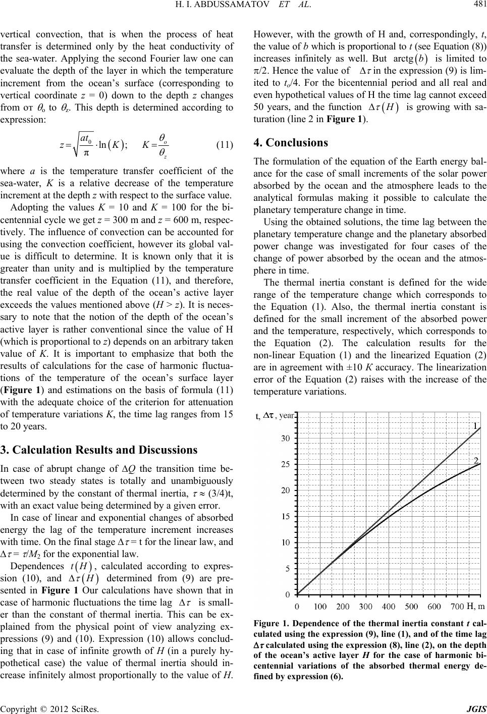
results of calculations for the case of harmonic fluctua-
tions of the temperature of the ocean’s surface layer
(Figure 1) and estimations on the basis of formula (11)
with the adequate choice of the criterion for attenuation
of temperature variations K, the time lag ranges from 15
to 20 years.
3. Calculation Results and Discussions
In case of abrupt change of Q the transition time be-
tween two steady states is totally and unambiguously
determined by the constant of thermal inertia,   (3/4)t,
with an exact value being determined by a given error.
In case of linear and exponential changes of absorbed
energy the lag of the temperature increment increases
with time. On the final stage   = t for the linear law, and
  =  /М2 for the exponential law.
Dependences , calculated according to expres-
sion (10), and
H
  determined from (9) are pre-
sented in Figure 1 Our calculations have shown that in
case of harmonic fluctuations the time lag



arctg b

is small-
er than the constant of thermal inertia. This can be ex-
plained from the physical point of view analyzing ex-
pressions (9) and (10). Expression (10) allows conclud-
ing that in case of infinite growth of H (in a purely hy-
pothetical case) the value of thermal inertia should in-
crease infinitely almost proportionally to the value of H.
However, with the growth of H and, correspondingly, t,
the value of b which is proportional to t (see Equation (8))
increases infinitely as well. But is limited to
/2. Hence the value of 
 in the expression (9) is lim-
ited to to/4. For the bicentennial period and all real and
even hypothetical values of H the time lag cannot exceed
50 years, and the function
H
  is growing with sa-
turation (line 2 in Figure 1).
4. Conclusions
The formulation of the equation of the Earth energy bal-
ance for the case of small increments of the solar power
absorbed by the ocean and the atmosphere leads to the
analytical formulas making it possible to calculate the
planetary temperature change in time.
Using the obtained solutions, the time lag between the
planetary temperature change and the planetary absorbed
power change was investigated for four cases of the
change of power absorbed by the ocean and the atmos-
phere in time.
The thermal inertia constant is defined for the wide
range of the temperature change which corresponds to
the Equation (1). Also, the thermal inertia constant is
defined for the small increment of the absorbed power
and the temperature, respectively, which corresponds to
the Equation (2). The calculation results for the
non-linear Equation (1) and the linearized Equation (2)
are in agreement with ±10 К accuracy. The linearization
error of the Equation (2) raises with the increase of the
temperature variations.
Figure 1. Dependence of the thermal inertia constant t cal-
culated using the expression (9), line (1), and of the time lag

 calculated using the expression (8), line (2), on the depth
of the ocean’s active layer H for the case of harmonic bi-
centennial variations of the absorbed thermal energy de-
fined by expression (6).

H. I. ABDUSSAMATOV ET AL.
482

f
The time lag dependence on the thermal inertia value
is estimated for each case of the

where the ther-
mal inertia is defined by the ocean active layer depth
(10).
The formula (11) is offered to estimate the ocean ac-
tive layer depth. The formula (11) leads to the conclusion
that in case of harmonic form of

f

the time lag
would range from 15 to 20 years.
Since the real bicentennial cyclic variations of the total
solar irradiance are not purely harmonic and contain dips
and glitches of 11-year cycles, the real time lag is deter-
mined by more complicated dependences. The changes
of can be caused also by long-term variations of
the Bond albedo. The character of its variations is poorly
understood so far, therefore both the linear and exponen-
tial presentations of the function
Q

f

can be used for
approximation of real variations during certain time in-
tervals.
REFERENCES
[1] M. I. Budyko, “The Effect of Solar Radiation Variations
on the Climate of Earth,” Tellus, Vol. 21, No. 5, 1969, pp.
611-619. doi:10.3402/2Ftellusa.v21i5.10109
[2] W. D. Sellers, “A Climate Model Based on the Energy
Balance of the Earth-Atmosphere System,” Journal of
Applied Meteorology and Climatology, Vol. 8, 1969, pp.
392-400.
doi:10.1175/2F1520-0450/281969%29008%3C0392%3A
AGCMBO%3E2.0.CO%3B2
[3] G. R. North, R. F. Cahalan and J. A. Coakley Jr., “Energy
Balance Climate Models,” Reviews of Geophysics, Vol.
19, No. 1, 1981, pp. 91-121.
doi:10.1029/2FRG019i001p00091
[4] C. E. Graves, W. Lee and G. R. North, “New Parameteri-
zation and Sensetivities for Simple Climate Models,”
Journal of Geophysical Research, Vol. 98, No. D3, 1993,
pp. 5025-5036. doi:10.1029/2F92JD02666
[5] J. I. Diaz, G. Hetzer and L. Tello, “An Energy Balance
Climate Model with Hysteresis,” Nonlinear Analysis, Vol.
64, No. 9, 2006, pp. 2053-2074.
doi:10.1016/2Fj.na.2005.07.038
[6] A. V. Karnaukhov, “Role of the Biosphere in the Forma-
tion of The Earth’s Climate: The Greenhouse Catastro-
phe,” Biophysics, Vol. 46, No. 6, 2001, pp. 1078-1088.
[7] B. G. Sherstyukov, “Thermal Inertia of the Ocean and the
Green-House Effect in the Modern Climate Variations,”
Meteorology and Hydrology, No. 7, 2006, pp. 66-72.
[8] H. I. Abdussamatov, A. Bogoyavlenskii, Y. V. Lapovok
and S. I. Khankov, “The Influence of the Atmospheric
Parameters Determining the Transparency of Solar and
Earth’s Radiation on the Climate,” Proceedings of the
All-Russian Annual Conference “Solar and Solar-Terre-
strial Physics—2010”, Saint-Petersburg, 2010, pp. 7-10.
[9] H. I. Abdussamatov, A. I. Bogoyavlenskii, Y.V. Lapovok
and S. I. Khankov, “Modeling of the Earth’s Planetary
Heat Balance with Electrical Circuit Analogy,” Journal of
Electromagnetic Analysis and Applications, Vol. 2, No. 3,
2010, pp. 133-138. doi:10.4236/jemaa.2010.23020
[10] H. I. Abdussamatov, A. I. Bogoyavlenskii, Y. V. Lapo-
vok and S. I. Khankov, “The Influence of the Atmos-
pheric Transmission for the Solar Radiation and Earth’s
Surface Radiation on the Earth’s Climate,” Journal of
Geographic Information System, Vol. 2, No. 10, 2010, pp.
194-200. doi:10.4236/jgis.2010.24027