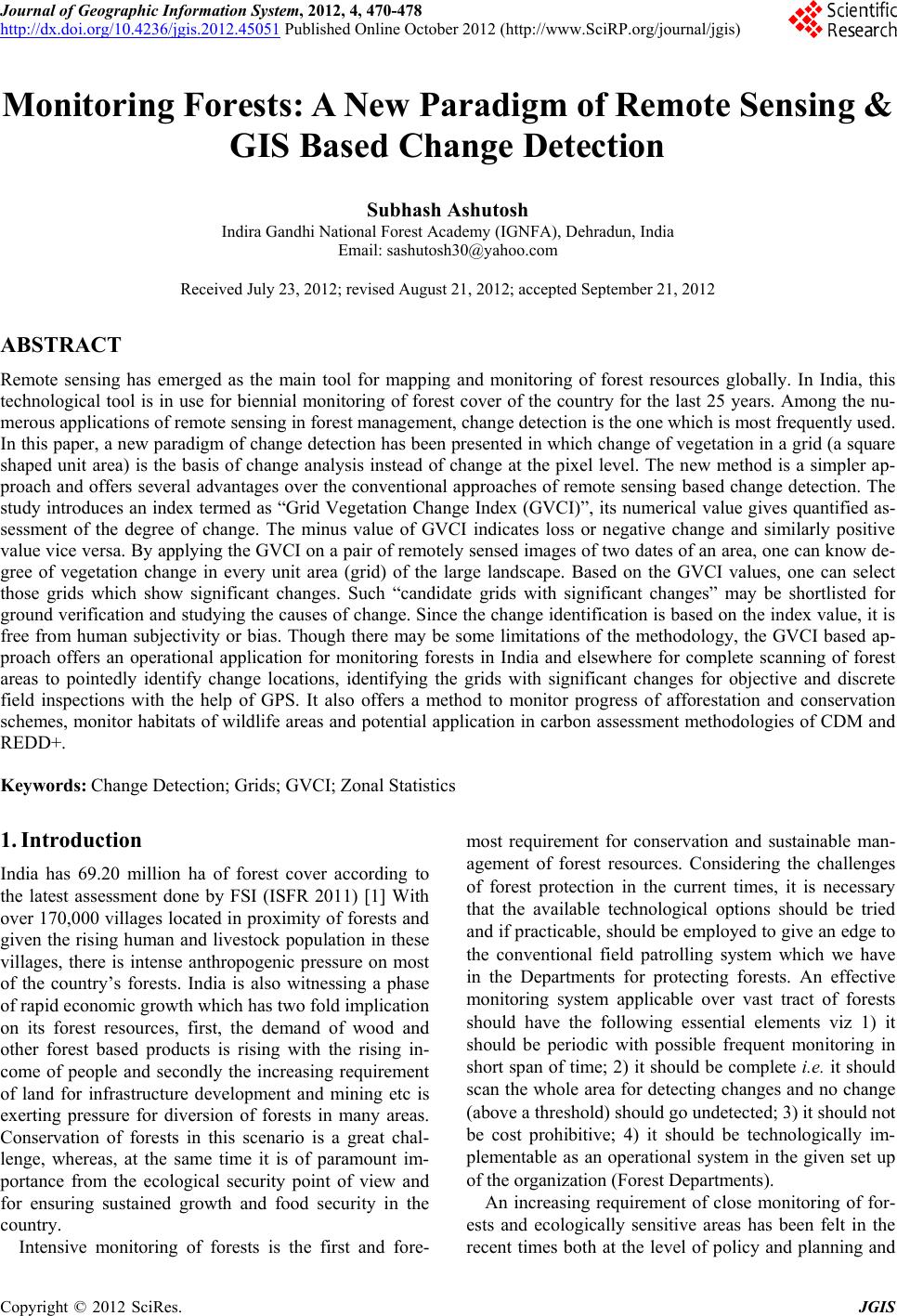Journal of Geographic Information System, 2012, 4, 470-478
http://dx.doi.org/10.4236/jgis.2012.45051 Published Online October 2012 (http://www.SciRP.org/journal/jgis)
Monitoring Forests: A New Paradigm of Remote Sensing &
GIS Based Change Detection
Subhash Ashutosh
Indira Gandhi National Forest Academy (IGNFA), Dehradun, India
Received July 23, 2012; revised August 21, 2012; accepted September 21, 2012
ABSTRACT
Remote sensing has emerged as the main tool for mapping and monitoring of forest resources globally. In India, this
technological tool is in use for biennial monitoring of forest cover of the country for the last 25 years. Among the nu-
merous applications of remote sensing in forest management, change detection is the one which is most frequently used.
In this paper, a new paradigm of change detection has been presented in which change of vegetation in a grid (a square
shaped unit area) is the basis of change analysis instead of change at the pixel level. The new method is a simpler ap-
proach and offers several advantages over the conventional approaches of remote sensing based change detection. The
study introduces an index termed as “Grid Vegetation Change Index (GVCI)”, its numerical value gives quantified as-
sessment of the degree of change. The minus value of GVCI indicates loss or negative change and similarly positive
value vice versa. By applying the GVCI on a pair of remotely sensed images of two dates of an area, one can know de-
gree of vegetation change in every unit area (grid) of the large landscape. Based on the GVCI values, one can select
those grids which show significant changes. Such “candidate grids with significant changes” may be shortlisted for
ground verification and studying the causes of change. Since the change identification is based on the index value, it is
free from human subjectivity or bias. Though there may be some limitations of the methodology, the GVCI based ap-
proach offers an operational application for monitoring forests in India and elsewhere for complete scanning of forest
areas to pointedly identify change locations, identifying the grids with significant changes for objective and discrete
field inspections with the help of GPS. It also offers a method to monitor progress of afforestation and conservation
schemes, monitor habitats of wildlife areas and potential application in carbon assessment methodologies of CDM and
REDD+.
Keywords: Change Detection; Grids; GVCI; Zonal Statistics
1. Introduction
India has 69.20 million ha of forest cover according to
the latest assessment done by FSI (ISFR 2011) [1] With
over 170,000 villages located in proximity of forests and
given the rising human and livestock population in these
villages, there is intense anthropogenic pressure on most
of the country’s forests. India is also witnessing a phase
of rapid economic growth which has two fold implication
on its forest resources, first, the demand of wood and
other forest based products is rising with the rising in-
come of people and secondly the increasing requirement
of land for infrastructure development and mining etc is
exerting pressure for diversion of forests in many areas.
Conservation of forests in this scenario is a great chal-
lenge, whereas, at the same time it is of paramount im-
portance from the ecological security point of view and
for ensuring sustained growth and food security in the
country.
Intensive monitoring of forests is the first and fore-
most requirement for conservation and sustainable man-
agement of forest resources. Considering the challenges
of forest protection in the current times, it is necessary
that the available technological options should be tried
and if practicable, should be employed to give an edge to
the conventional field patrolling system which we have
in the Departments for protecting forests. An effective
monitoring system applicable over vast tract of forests
should have the following essential elements viz 1) it
should be periodic with possible frequent monitoring in
short span of time; 2) it should be complete i.e. it should
scan the whole area for detecting changes and no change
(above a threshold) should go undetected; 3) it should not
be cost prohibitive; 4) it should be technologically im-
plementable as an operational system in the given set up
of the organization (Forest Departments).
An increasing requirement of close monitoring of for-
ests and ecologically sensitive areas has been felt in the
recent times both at the level of policy and planning and
C
opyright © 2012 SciRes. JGIS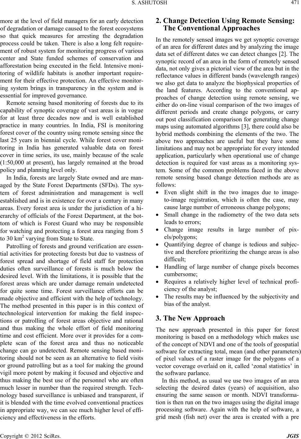

S. ASHUTOSH 471
more at the level of field managers for an early detection
of degradation or damage caused to the forest ecosystems
so that quick measures for arresting the degradation
process could be taken. There is also a long felt require-
ment of robust system for monitoring progress of various
center and State funded schemes of conservation and
afforestation being executed in the field. Intensive moni-
toring of wildlife habitats is another important require-
ment for their effective protection. An effective monitor-
ing system brings in transparency in the system and is
essential for improved governance.
Remote sensing based monitoring of forests due to its
capability of synoptic coverage of vast areas is in vogue
for at least three decades now and is well established
practice in many countries. In India, FSI is monitoring
forest cover of the country using remote sensing since the
last 25 years in biennial cycle. While forest cover moni-
toring in India has generated valuable data on forest
cover in time series, its use, mainly because of the scale
(1:50,000 at present), has largely remained at the broad
policy and planning level only.
In India, forests are largely State owned and are man-
aged by the State Forest Departments (SFDs). The sys-
tem of forest administration and management is well
established and is in existence for over a century in many
areas. Every forest area is under the jurisdiction of a hi-
erarchy of officials of the Forest Department, at the bot-
tom of which is Forest Guard who may be responsible
for watching and protecting a forest area ranging from 5
to 30 km2 varying from State to State.
Patrolling of forests and ground verification are essen-
tial activities for protecting forests but due to vastness of
forest spread and shortage of field staff for protection
duties often surveillance of forests is much below the
desired level. With the limitations, it is possible that the
forest areas which are under damage remain undetected
for quite some time. Forest surveillance efforts can be
made objective and efficient with the help of technology.
The method presented in this paper is in this context of
technological intervention for making the field inspec-
tions or patrolling of forest areas objective and rational
and thus making the whole effort of field monitoring
time and cost efficient. More over it provides for a com-
plete scan of the forest area and thus no noticeable
change can go undetected. Remote sensing based moni-
toring should not be seen as an alternative to field visits
or ground patrolling but as a tool for making the ground
vigil more potent by making it focused and objective and
thus making the best use of the personnel who are often
much lesser in number than the required strength. Tech-
nology based surveillance is unbiased and transparent, if
it is blended with the time evolved conventional practices
in appropriate way, we can see much higher level of effi-
ciency and effectiveness in the efforts.
2. Change Detection Using Remote Sensing:
The Conventional Approaches
In the remotely sensed images we get synoptic coverage
of an area for different dates and by analyzing the image
data set of different dates we can detect changes [2]. The
synoptic record of an area in the form of remotely sensed
data, not only gives a pictorial view of the area but in the
reflectance values in different bands (wavelength ranges)
we also get data to analyze the biophysical properties of
the land features. According to the conventional ap-
proaches of change detection using remote sensing, we
either do on-line visual comparison of the two images of
different periods and create change polygons, or carry
out post classification comparison for generating change
maps using automated algorithms [3], there could also be
hybrid methods combining the elements of the two. The
above two approaches are useful but they have some
limitations and may not be appropriate for every intended
application, particularly when operational use of change
detection is required for vast areas as a monitoring sys-
tem. Some of the common problems faced in the above
remote sensing based change detection methods are as
follows:
 Even slight shift in the two images due to image-
to-image registration, which is often the case, may
cause large number of erroneous change polygons;
 Small change in the radiometry of the two data sets
leads to errors;
 Change image results in large number of pix-
els/polygons;
 Quantifying degree of change is tedious and subjec-
tive and therefore prioritizing the change areas is also
difficult;
 Handling of large number of change pixels becomes
cumbersome;
 Requires a relatively higher level of technical profi-
ciency of the analyst;
 The results may be influenced by the subjectivity and
bias of the analyst.
3. The New Approach
The new approach presented in this paper for forest
monitoring is based on a methodology which makes use
of the concept of NDVI and one of the tools of geospatial
software for extracting total, mean (and other parameters)
of pixel values of a raster image for the polygons of a
vector coverage overlaid on it, called ‘zonal statistics’ in
the software parlance.
In this method, as usual we use two images of an area
selecting the desired dates (years) of acquisition, also
ensuring the same season or month. NDVI transforma-
tion is then run on the two images using the digital image
processing software. Again with the help of software, a
grid mesh (fish net) over the area is created with a pre

S. ASHUTOSH
472
decided grid size. Grid size is to be decided based on the
resolution of the satellite data and the unit ground area
for which changes are to be monitored, say 500 m × 500
m (25 ha) or 1 km × 1 km (100 ha) with IRS P6 LISS III
data. A grid should include sufficiently large number of
pixels for providing robustness to the index value and at
the same time its size should be such that the ground
verification could be done in a practicable way. The steps
of the methodology are given as follows:
In the Zonal Statistics based approach presented in this
study, comparison of NDVI of the two images has been
done for grid polygons of uniform sizes (say 500 m ×
500 m - 25 ha) which have been created using “fishnet”
feature of the Arc GIS software.
 NDVI images of the two periods are generated.
 Zonal statistics of mean NDVI of all the grids for
both the images are generated.
 Mean values of NDVI of the two images are stretched
between 0 and 1using global minimum and global
maximum values (for uniformity and standardized
application for comparing two different dates of im-
ages).
 It was observed that stretching of NDVI values be-
tween 0 and 1 minimizes the changes due to differ-
ence in radiometry of the two images which may arise
on account of various atmospheric, weather and sen-
sor related factors.
 Using the above mean and stretched values of NDVI
(transformed NDVI) for each grid, an index is derived
which gives the percent change in the transformed
NDVI values between the corresponding grids.
 The index which may be termed as Grid Vegetation
Change index (GVCI) can be mathematically ex-
pressed as follows.
A “grid vegetation change index (GVCI)” Ij has been
defined as the percentage change in the mean values of
NDVI for each grid which can be derived by the follow-
ing formula


21
100 MM
jjt

1
M
jtjt
I
NDVI NDVI NDVI
 
(1)
where 1
M
j
t
NDVI and 2
M
j
t are the mean values of
NDVI of jth grid at time t1 and t2 respectively
NDVI
M
NDVI 
jji
iNDVI n
 (2)
where
j
i is the NDVI value of ith pixel in jth grid
and n is the total number of pixels in the grid
NDVI
M
NDVI  is the stretched value of
M
NDVI between
0 and 1 taking “global max” and “global min” values of
M
NDVI of the study area into account.



min
min
global
MM
global
VI
max
MM
M
global
NDVI NDVI
NDVI NDVI ND

 (3)
The above defined Grid Vegetation Change Index
(GVCI) is an operational index which significance in
terms of biophysical properties has not been studied. This
is expected to reflect percentage change in the average
NDVI values of a grid between two dates and thus would
be correlated to the physical significance of NDVI in a
general way.
4. Work-Flow
The work-flow is shown in Figure 1.
4.1. Advantages of the Zonal Statistics Based
Approach
 Provides a robust methodology for identifying areas
of forest change between two dates for vast land-
scapes in a short time;
 An automated approach, free from subjectivity of the
interpreter;
 Numerical value of the index gives clear indication of
the degree of change;
 Error due to image registration is minimized;
 Impact of radiometric differences in the images due to
atmospheric or other factors in identifying change is
also minimized;
 Change is given in terms of numerical values of the
index (GVCI);
 Gives a complete scan of the area, it is normally not
possible that a change above certain threshold goes
undetected;
 Change areas can be prioritized using the numerical
value of the index for the desired action on the ground.
4.2. What Makes the Approach Robust?
 The index is based on DN values of many pixels
(more than 100) and therefore the average of NDVI in
a grid (say of size 25 ha) gives a robust parameter
about the amount and health of vegetation in that
small area.
 With ratio operating at three stages in the index (i.e.
NDVI, stretch and percentage), atmospheric and ra-
diometric factors of multiplicative nature which are
the potential source of errors get minimized.
 The index also involves minus operation and thus
minimizes errors of additive nature.
 The unit area (of observation) becomes an average of
many individual pixels and therefore geometric error
of pixel level in image registration has lesser conse-
quence in identifying change in the unit area.
4.3. Unit Area of Observation (Grid)
Size of unit area of observation i.e. a grid in this method-
ology may be chosen considering the objectives of
monitoring and the pixel size of the satellite data being
used. Each grid is identifiable by a unique Id. The size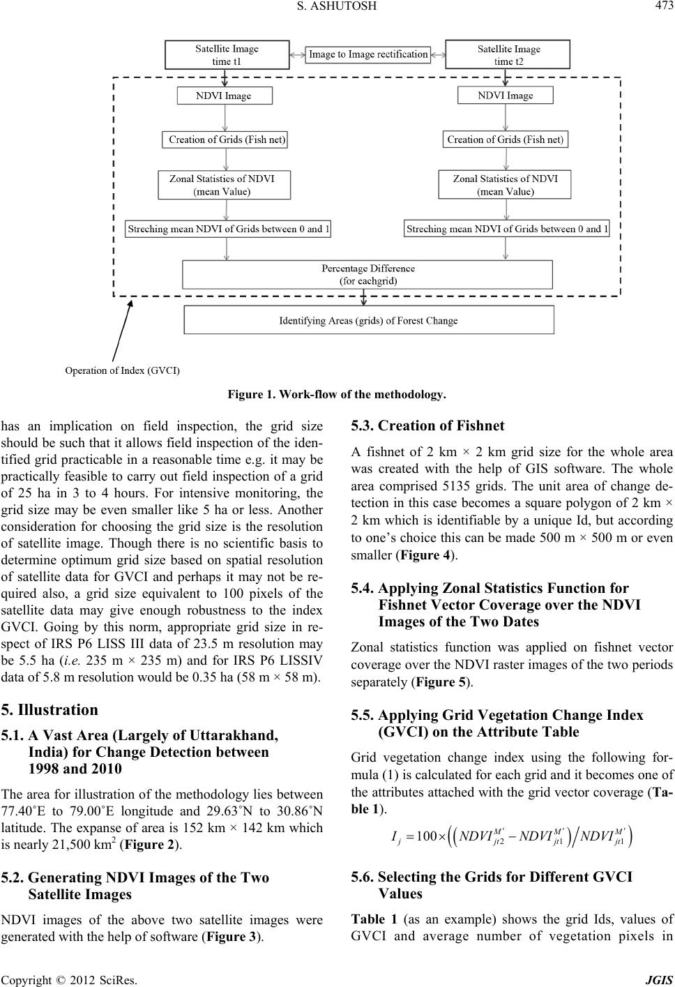

S. ASHUTOSH
473
Figure 1. Work-flow of the methodology.
5.3. Creation of Fishnet
has an implication on field inspection, the grid size
should be such that it allows field inspection of the iden-
tified grid practicable in a reasonable time e.g. it may be
practically feasible to carry out field inspection of a grid
of 25 ha in 3 to 4 hours. For intensive monitoring, the
grid size may be even smaller like 5 ha or less. Another
consideration for choosing the grid size is the resolution
of satellite image. Though there is no scientific basis to
determine optimum grid size based on spatial resolution
of satellite data for GVCI and perhaps it may not be re-
quired also, a grid size equivalent to 100 pixels of the
satellite data may give enough robustness to the index
GVCI. Going by this norm, appropriate grid size in re-
spect of IRS P6 LISS III data of 23.5 m resolution may
be 5.5 ha (i.e. 235 m × 235 m) and for IRS P6 LISSIV
data of 5.8 m resolution would be 0.35 ha (58 m × 58 m).
A fishnet of 2 km × 2 km grid size for the whole area
was created with the help of GIS software. The whole
area comprised 5135 grids. The unit area of change de-
tection in this case becomes a square polygon of 2 km ×
2 km which is identifiable by a unique Id, but according
to one’s choice this can be made 500 m × 500 m or even
smaller (Figure 4).
5.4. Applying Zonal Statistics Function for
Fishnet Vector Coverage over the NDVI
Images of the Two Dates
Zonal statistics function was applied on fishnet vector
coverage over the NDVI raster images of the two periods
separately (Figure 5).
5. Illustration 5.5. Applying Grid Vegetation Change Index
(GVCI) on the Attribute Table
5.1. A Vast Area (Largely of Uttarakhand,
India) for Change Detection between
1998 and 2010 Grid vegetation change index using the following for-
mula (1) is calculated for each grid and it becomes one of
the attributes attached with the grid vector coverage (Ta-
ble 1).
The area for illustration of the methodology lies between
77.40˚E to 79.00˚E longitude and 29.63˚N to 30.86˚N
latitude. The expanse of area is 152 km × 142 km which
is nearly 21,500 km2 (Figure 2).




21 1
100 MMM
jjtjtjt
5.2. Generating NDVI Images of the Two
Satellite Images
NDVI images of the above two satellite images were
generated with the help of software (Figure 3).
I
NDVI NDVINDVI


 
5.6. Selecting the Grids for Different GVCI
Values
Table 1 (as an example) shows the grid Ids, values of
GVCI and average number of vegetation pixels in

S. ASHUTOSH
474
LANDSAT TM Image 12th Nov, 1998 LANDSAT TM Image 12th Nov, 2010
Figure 2. Satellite images of the study area for two dates.
Figure 3. NDVI image of the study area.
Figure 4. Fishnet over the study area.

S. ASHUTOSH 475
Figure 5. Zonal statistics template.
Table 1. Grid Ids, index values and average sum of vegetation pixels (extent of vegetation in the grid)—part only.
Grid_Id GVCI Average Sum of Vegetation Pixels
1000 –1.137 155.856
1001 –4.023 147.055
1002 –1.820 154.738
1003 –1.105 152.316
1004 –1.085 141.402
1005 –0.049 152.935
1006 –1.471 154.213
1007 –1.108 143.689
1008 0.446 145.764
1009 –10.089 144.521
1010 –10.571 130.026
1011 –10.749 108.769
1012 –21.669 25.909
1013 –5.073 6.605
1014 –8.450 24.498
1015 –1.839 159.181
1016 –1.311 144.523
1017 2.261 150.984
1018 4.087 153.793
1019 4.443 145.125
1020 5.005 153.985
contd.
the grids i.e. the extent of vegetation cover. The grid Id
1012 shows the maximum change which is negative but
the grid has low area under vegetation. The grids with Ids
1009 and 1010 also show significant negative change and
have good extent of vegetation. The grid Id 1020 shows
positive change (improvement) and has good vegetation
cover. Selection of grids and display of change on the
computer screen based on the criteria of one’s choice can
be easily done with the GIS software. Product of the
GVCI and “average sum of vegetation pixels” will give

S. ASHUTOSH
476
an indicative measure of total vegetation change in a grid.
The total of the product for all the grids will give a
measure of total vegetation change in a given study area.
The change analysis of the above area using 2 km × 2
km grids has shown number of grids in different degree
of vegetation change in terms of the GVCI values. The
negative changes or losses is shown by the negative val-
ues, whereas, the gains or positive changes in the vegeta-
tion are shown by the positive values of GVCI (Table 1).
Table 2 shows that out of total 5395 grids in the study
area, 4016 (74.4%) grids show loss in vegetation during
the period 1998 and 2010 and only 1379 (25.6%) grids
show gain in vegetation. Thus the area selected for illus-
tration shows over all negative change in the vegetation.
As illustrated above one can use GVCI values in se-
lecting the “candidate grids with significant changes”
which may be above (or lower in case of negative
changes) certain threshold value of GVCI. Such grids
may then be field inspected for ascertaining ground de-
tails and studying the reasons of change.
5.7. Visualization of Changes in the Grids
Selected by GVCI Values
The above procedure was applied on several pairs of re-
mote sensing Images of different areas and in every case
the above methodology effectively highlighted signifi-
cant change areas on images spanning over areas 5000 to
15,000 km2 (Figure 6).
6. Limitations
1) The GVCI works well in highlighting the grids
where vegetation change has taken place, though some-
times atmospheric conditions like haze and clouds etc.
Table 2. Summary of GVCI values showing overall changes
in the study area.
GVCI Values No. of Grids
less than −40 361
between −40 and −30 272
between −30 and −20 282
between −20 and −10 570
between −10 and 0 2531
between 0 and 10 1335
between 10 and 20 24
between 20 and 30 4
between 30 and 40 5
Greater than 40 11
Total 5395
November 1998 GVCI = –28.11 November 2010
(a)
November 1998 GVCI = –35.89 November 2010
(b)

S. ASHUTOSH 477
November 1998 GVCI = –21.91 November 2010
(c)
November 1998 GVCI = –43.24 November 2010
(d)
November 1998 GVCI = +14.71 November 2010
(e)
Figure 6. Illustration of changes.
obscure the real change in vegetation and the change
highlighted by the index in a grid may be influenced by
these atmospheric factors. This limitation can be over-
come to a great extent by preprocessing of satellite data
for atmospheric correction.
2) Radiometric variations in the satellite images due to
changes in satellite ephemeris, illumination conditions or
aging of the satellite/sensor would affect the GVCI val-
ues to some extent and thus influence the detection of
forest change.
3) Changes in the deep shadow areas are not detected.
4) It is necessary that the two time satellite images
used in the change detection by above approach should
be from the same season (month of the year).
7. Conclusion
The methodology presented in this paper is a new remote
sensing based approach for scanning vast landscapes for
detecting changes in forests or other vegetation forms in
a pointed manner, highlighting small square tiles (say 25
ha or smaller) where change in forest/vegetation has
taken place. The paper introduces a new index (GCVI)
based on NDVI and a spatial feature of GIS software
(computing zonal attributes) for detection of changes in
forests. The method can be effectively used in making
the ground inspections objective and in identifying sensi-

S. ASHUTOSH
478
tive areas for taking effective measures for arresting the
causes of any degradation process. It should not be seen
as an alternative to the field patrolling based surveillance
of forests, rather this method coupled with field patrol-
ling can make the effort much more effective. Quantifi-
cation of change by this method can help in prioritizing
the areas for intense monitoring. The approach can also
be used in monitoring implementation of afforestation
and conservation activities under various schemes. This
methodology can be practicably implemented in the State
Forest Departments with one centralized system moni-
toring a large forest area on a desired periodicity.
8. Acknowledgements
The author gratefully acknowledges support and encour-
agement given by Director, IGNFA and help rendered by
Smt Pushpalatha Devala, Technical Associate. The study
was carried out in the Geomatics Lab of IGNFA.
REFERENCES
[1] Forest Survey of India, India State of Forest Report
(ISFR), 2009.
[2] A. J. Elmore, J. F. Mustard, S. J. Manning and D. B. Lo-
bell, “Quantifying Vegetation Change in Semiarid Envi-
ronments: Precision and Accuracy of Spectral Mixture
Analysis and the Normalized Difference Vegetation In-
dex,” Remote Sensing of Environment, Vol. 73, No. 1,
2000, pp. 87-102.
[3] J. G. Lyon, D. Yuan, R. S. Lunetta and C. D. Elvidge, “A
Change Detection Experiment Using Vegetation Indices,”
Photogrammetric Engineering & Remote Sensing, Vol.
64, No. 2, 1998, pp. 143-150.