Advances in Chemical Engineering and Science, 2012, 2, 481-489
http://dx.doi.org/10.4236/aces.2012.24059 Published Online October 2012 (http://www.SciRP.org/journal/aces)
Conceptual Modeling of Contaminated Solute Transport
Based on Stream Tube Model
Seung-Gun Chung1,2, Soon-Jae Lee1,2, Dong-Ju Kim2, Sang-Hyup Lee1, Jae-Woo Choi1*
1Center for Water Resource Cycle Research, Korea Institute of Science and Technology, Seoul, South Korea
2Department of Earth and Environmental Sciences, College of Science, Korea University, Seoul, South Korea
Email: *plead36@kist.re.kr
Received July 28, 2012; revised August 30, 2012; accepted September 9, 2012
ABSTRACT
In this study, we performed a conceptual modeling on solute transport based on theoretical stream tube model (STM)
with various travel time distributions assuming a pure convective flow through each tube in order to investigate how the
lengths and distributions of solute travel time through STM affect the breakthrough curves at the end mixing surface.
The conceptual modeling revealed that 1) the shape of breakthrough curve (BTC) at the mixing surface was determined
by not only input travel time distributions but also solute injection mode such as sampling time and pulse lengths; 2) the
increase of pulse length resulted in the linear increase of the first time moment (mean travel time) and quadratic in-
crease of the second time moment (variance of travel time) leading to more spreading of solute, however, the second
time moment was not affected by travel time distributions; and 3) for a given input distributions the increase in travel
distance resulted in more dispersion with the quadratic increase of travel time variance. This indicates that stream tube
model obeying strictly pure convective flow follows the concept of convective-lognormal transport (CLT) model re-
gardless the input travel time distributions.
Keywords: Conceptual Modeling; Solute Transport; Pure Convective Flow; Stream Tube Model; Travel Time
Distribution
1. Introduction
At macroscopic scale, there are three basic causes of ve-
locity difference in pore-water that are friction loss, dif-
ferences in pore size and path length, all or each of which
leads to mixing of solute and thereby brings about me-
chanical dispersion [1]. This mechanical dispersion is
considered as a key parameter responsible for mixing or
dilution of solutes during transport through soils and dis-
tinguished from molecular diffusion arising from density
or concentration differences. Combination of mechanical
dispersion with molecular diffusion is termed hydrody-
namic dispersion which constitutes major transport pa-
rameters of solute transport equation together with con-
vection. For instance, the convection-dispersion equation
(CDE) of solute transport for nonreactive solute is de-
scribed by only these two parameters. It is, however,
based on a set of assumptions that are likely to be valid
only under certain conditions in soil or aquifer systems.
The CDE makes the hypothesis that the dispersion proc-
ess is formally equivalent to diffusion even though dis-
persion is a convective transport process.
Because the CDE is valid only after sufficient time has
elapsed to smooth out transport by convective velocity
differences along the direction of motion, it cannot be
valid at early times. For this reason, Jury [2] developed
an alternative formulation for solute transport, called the
transfer function or convective lognormal transfer func-
tion (CLT) model, which does not require the restrictive
assumptions of the CDE and can be applied to problems
at different scales. This model relates an input condition
to the output variable of interest based on the assumption
that the velocity of a solute particle remains constant
along its travel path through the soil. It further assumes
that there is no exchange of solute particles between
pores with different water velocities. In this regard, sol-
ute particle arrival times are perfectly correlated with
lognormal distribution of pore water velocities and solute
travel time variance increases quadratically with depth.
Recently Bardsley [3] studied temporal moments of a
tracer pulse in a perfectly parallel flow system by parti-
tioning water flow into isolated one-dimensional stream
tubes which maintain spatial correlation of all properties
in the direction of flow. The individual flow tubes in the
parallel flow model are referred to as channels for frac-
ture-flow and layers in the context of perfectly stratified
aquifer systems.
*Corresponding author.
C
opyright © 2012 SciRes. ACES
S.-G. CHUNG ET AL.
482
Tracer transport in parallel systems provides a non-
diffusive mechanism contributing to dispersion [4-8].
This stream tube effect has been referred to as a convec-
tive-dispersive process [9,10], causing tracer arrival-time
variance to increase as a quadratic function of travel dis-
tance for convective flow. Since within a single stream
tube all hydraulic properties remain constant, the distri-
bution of travel time or flow velocities between stream
tubes will be the utmost important factors determining
the dispersive process at the outflow mixing surface. In
the previous studies of dispersion, the effect of normal
distributions [11,12], normal or lognormal arrival times
[10,13,14] between the stream tubes on solute transport
were investigated. However, to date there has been no
systematic study on both a pure convective process
within a stream tube and the effect of normal or log-
normal distributions of arrival times between stream
tubes on solute transport. In addition to the travel time
distributions, there would be some other factors such as
sampling time and pulse duration which influence the
dispersive process for pure convective flow.
The objective of this study is (1) to generate the break-
through curves (BTC) of nonreactive solute using a con-
ceptual stream tube model (STM) by assuming pure
convective process and (2) to investigate how the pulse
conditions and various travel time distributions affect the
transport concept of stream tube model using time mo-
ment analysis.
2. Material and Methods
2.1. Modeling of Conceptual Stream Tube
The conceptual stream tube model can be constructed in
two different ways. The first is a diameter-based type to
assemble a finite number of tubes with equal lengths but
different cross-sectional areas or diameters so that dif-
ferent average flow velocities are achieved by allowing
equal flow rate to each tube. The other is a length-based
type to construct the tubes with equal diameter but dif-
ferent lengths in order for the stream tubes to have nor-
mal or lognormal distributions of travel time when an
equal amount of discharge is imposed to each tube. In
this study, the latter case is adopted.
Following assumptions should be made for the con-
ceptual stream tube model:
1) The stream tube model is constructed with a finite
number of bundles of one-dimensional stream tubes with
equal diameter but different lengths.
2) Flow velocity within a single tube is steady and in-
variant.
3) Tracer solution is injected uniformly at the inlet
boundary of each tube.
4) Tracer transport in each tube obeys the convective
flow.
5) Molecular diffusion during pulse input is neglected.
6) Dispersive mixing occurs due to velocity differences
between tubes at the outflow mixing surface by instanta-
neous and complete mixing.
7) Effluents are collected at one common mixing sur-
face regardless the differences in tube lengths.
8) Velocity differences can be realized by normal or
lognormal distributions of travel length or time.
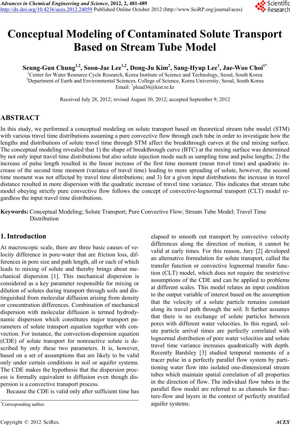
Consider a set of stream tubes which has a normal dis-
tribution of tube length as shown in Figure 1 where each
bundle consisting of the same tube length has a different
tube number. Let the length of ith tube bundle be Li, the
number of ith tube bundle Ni. Then the total number of
max
1
i
i
i
NTT N
. Let the diameter and cross- tubes is
sectional area of each tube be d and A, and injection flow
rate at the inlet boundary Q, injection concentration Co,
pulse duration To. Then the flow velocity and flow rate in
each tube is
vQNTTA
,
qQNTT
LvT and pulse
length 0p
t
. If a STM consists of five different
lengths (30, 40, 50, 60, 70 cm) and sampling time inter-
val Lvt
, then the sampling length interval

and number of pulse length p. Let the
number of sampling J and then sampling time will be
NPL LL
12
J
TJ t

L. For instance, the number of times of
which can have the effluent concentration for ith
bundle ii
TLLL, and the number of times of
required for breakthrough of ith tube ii
TT .
Then the number of tubes with tracer effluent at sampling
time J would be the following:
T NPL

where
J
iii
iI
NTENIi TJTT

(1)
Therefore the effluent concentration at J will be
00
J
J
J
qtNTE NTE
CC C
Qt NTT
 


L
(2)
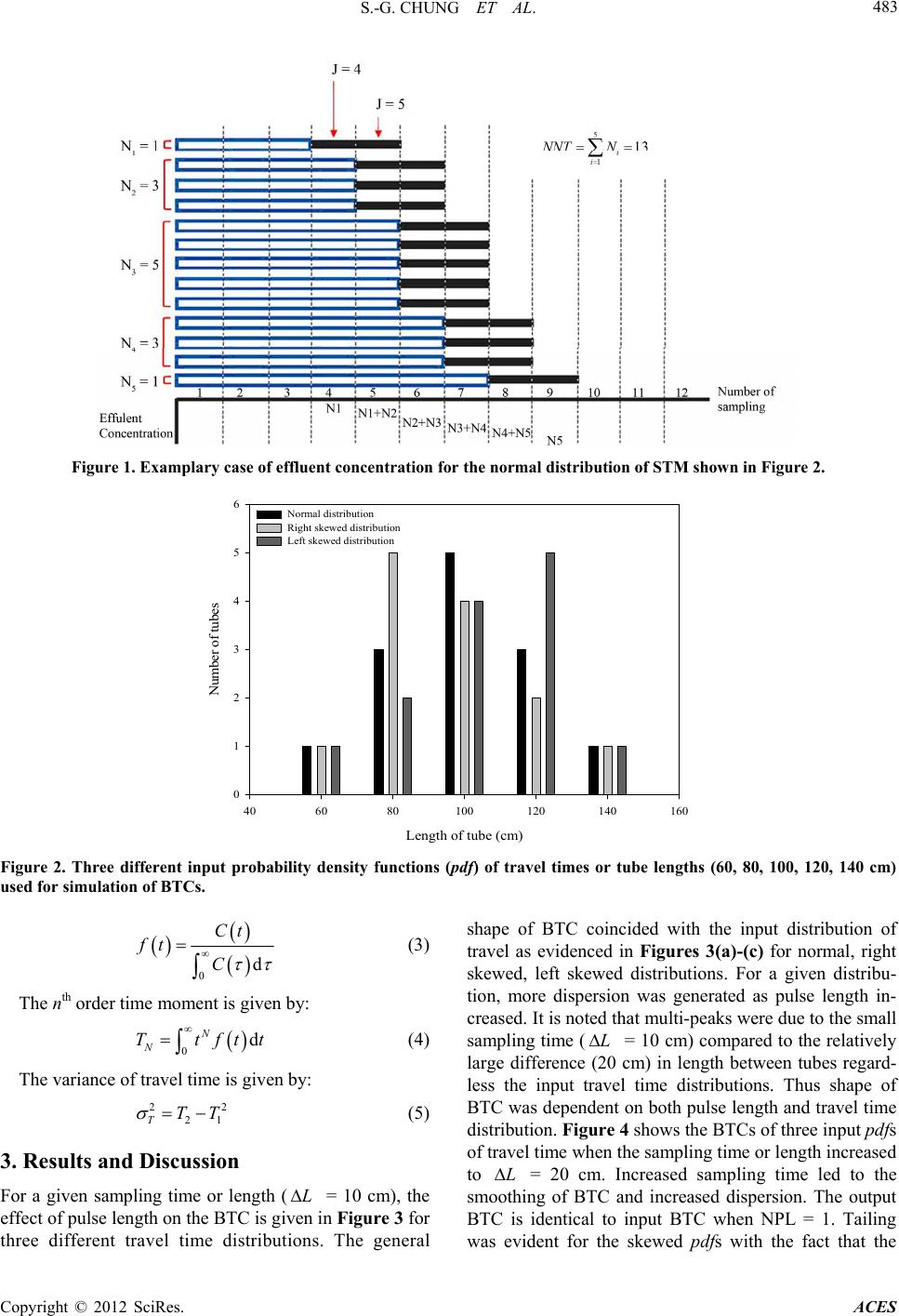
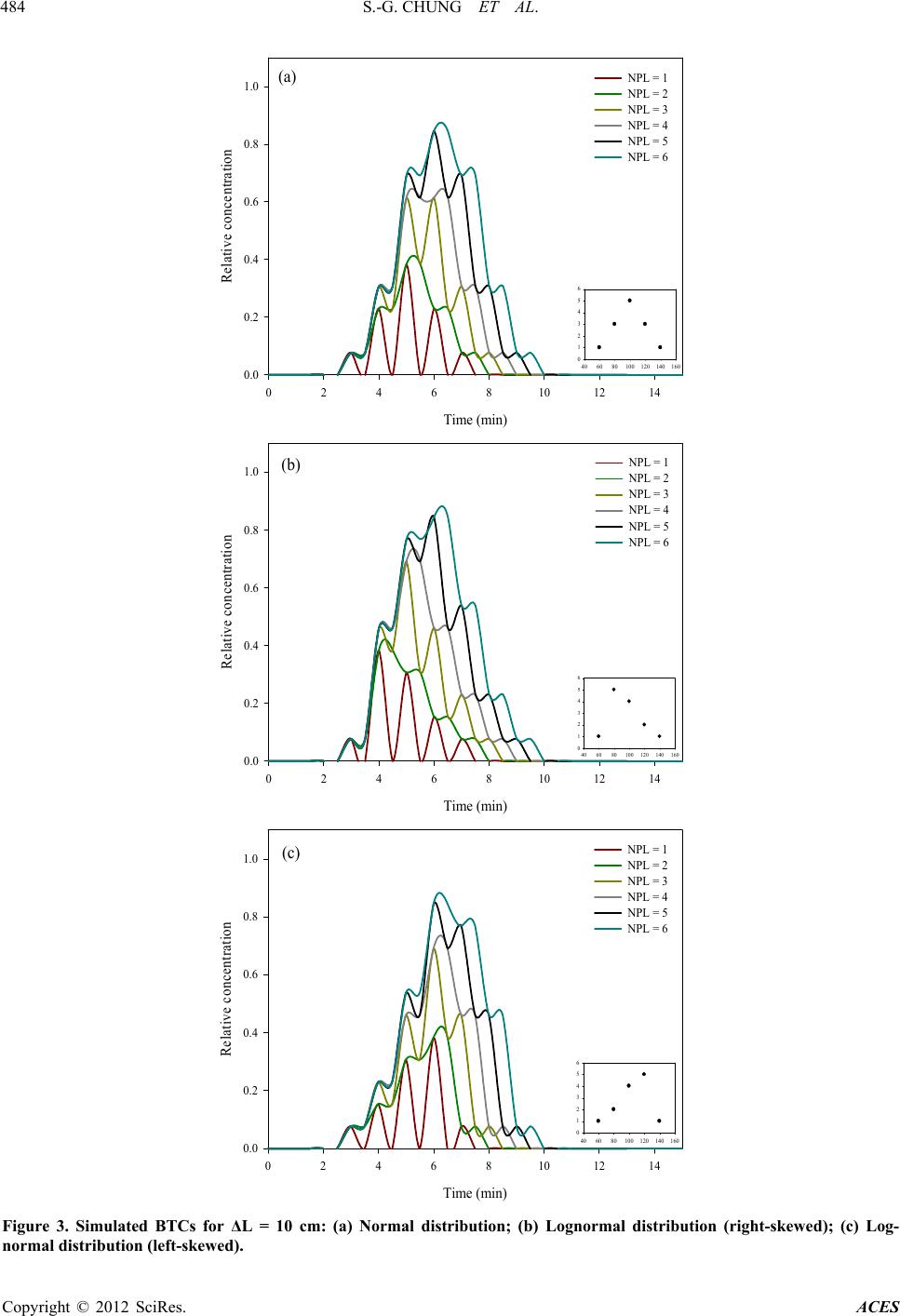
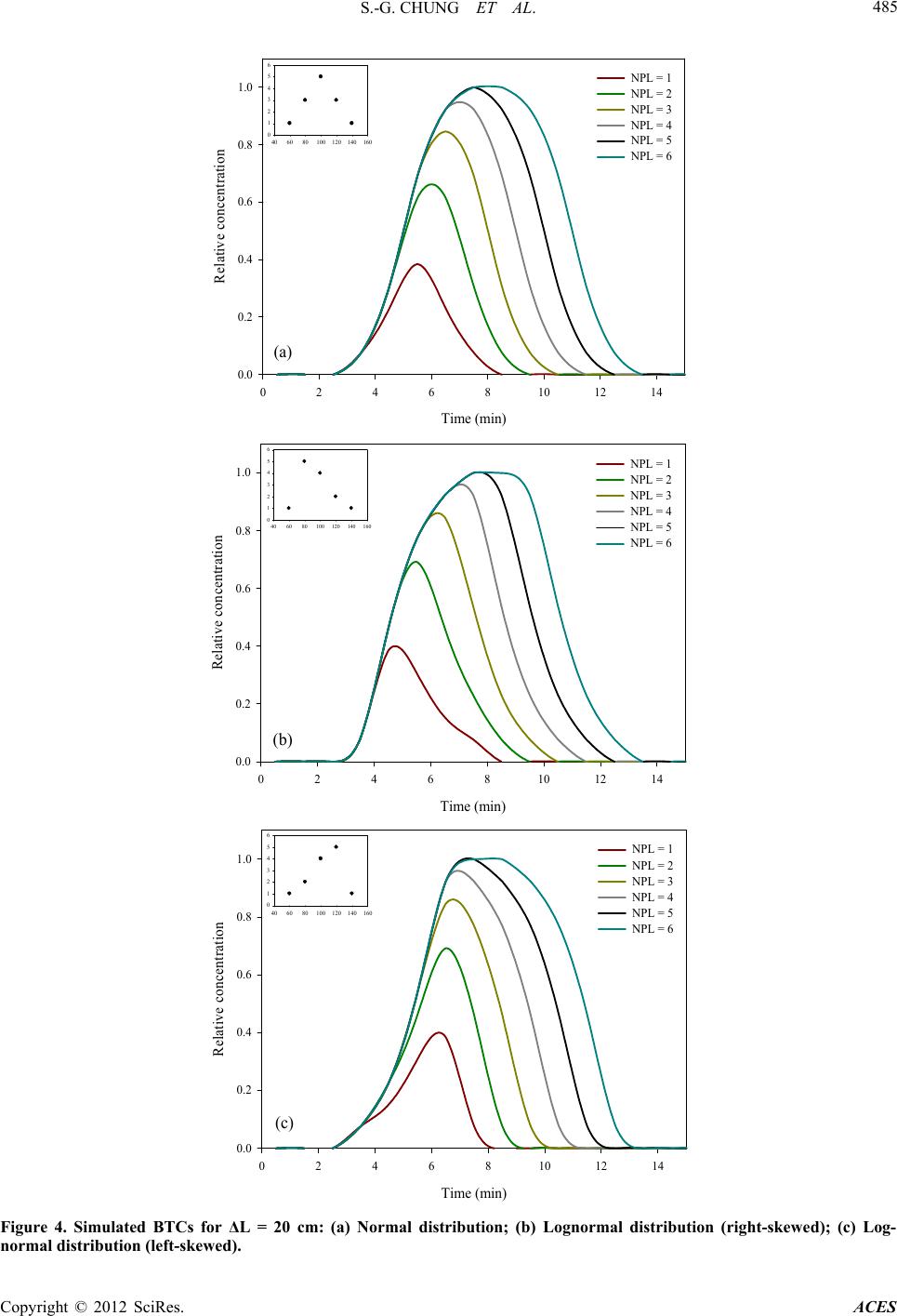
In order to investigate the effect of travel time distri-
bution on the convective-dispersive process, we gener-
ated three different input probability density functions of
travel times or tube lengths (60, 80, 100, 120, 140 cm) as
was shown in Figure 2 and used them for simulation of
BTCs at the mixing surface based on pure convective
flow within stream tubes. Sensitivity analysis was also
performed to see the effect of sampling time (
= 10,
20 cm) and pulse length (NPL = 1 to 6) on the BTCs.
2.2. Time Moment Analysis
In order to investigate the effect of sampling time, pulse
duration and input distribution of travel length on the
dispersive process along stream tubes, time moment
analysis was performed. The simulated concentrations in
time were first converted to probability density function
(pdf) as:
Copyright © 2012 SciRes. ACES
S.-G. CHUNG ET AL.
Copyright © 2012 SciRe ACES
483
Figure 1. Examplary case of effluent concentration for the normal distribution of STM shown in Figure 2.
Length of tube (cm)
406080100 120 140 160
Number of tubes
0
1
2
3
4
5
6
Normal distribution
Right skewed distribution
Left skewed distribution
Figure 2. Three different input probability density functions (pdf) of travel times or tube lengths (60, 80, 100, 120, 140 cm)
used for simulation of BTCs.

s.

0d
Ct
C
ft

0d
N
Ttftt
22
21TTT

L
L
(3)
The nth order time moment is given by:
N (4)
The variance of travel time is given by:
(5)
3. Results and Discussion
For a given sampling time or length ( = 10 cm), the
effect of pulse length on the BTC is given in Figure 3 for
three different travel time distributions. The general
shape of BTC coincided with the input distribution of
travel as evidenced in Figures 3(a)-(c) for normal, right
skewed, left skewed distributions. For a given distribu-
tion, more dispersion was generated as pulse length in-
creased. It is noted that multi-peaks were due to the small
sampling time (
= 10 cm) compared to the relatively
large difference (20 cm) in length between tubes regard-
less the input travel time distributions. Thus shape of
BTC was dependent on both pulse length and travel time
distribution. Figure 4 shows the BTCs of three input pdfs
of travel time when the sampling time or length increased
to L
= 20 cm. Increased sampling time led to the
smoothing of BTC and increased dispersion. The output
BTC is identical to input BTC when NPL = 1. Tailing
was evident for the skewed pdfs with the fact that the
S.-G. CHUNG ET AL.
484
Time (min)
02468101214
Relative concentration
0.0
0.2
0.4
0.6
0.8
1.0 NPL = 1
NPL = 2
NPL = 3
NPL = 4
NPL = 5
NPL = 6
406080100 120140 160
0
1
2
3
4
5
6
(a)
Time (min)
02468101214
Relative concentration
0.0
0.2
0.4
0.6
0.8
1.0 NPL = 1
NPL = 2
NPL = 3
NPL = 4
NPL = 5
NPL = 6
406080100 120 140160
0
1
2
3
4
5
6
(b)
Time (min)
02468101214
Relative concentration
0.0
0.2
0.4
0.6
0.8
1.0 NPL = 1
NPL = 2
NPL = 3
NPL = 4
NPL = 5
NPL = 6
406080100 120 140 160
0
1
2
3
4
5
6
(c)
Figure 3. Simulated BTCs for ΔL = 10 cm: (a) Normal distribution; (b) Lognormal distribution (right-skewed); (c) Log-
normal distribution (left-skewed).
Copyright © 2012 SciRes. ACES
S.-G. CHUNG ET AL. 485
Time (min)
02468101214
Relative concentration
0.0
0.2
0.4
0.6
0.8
1.0 NPL = 1
NPL = 2
NPL = 3
NPL = 4
NPL = 5
NPL = 6
406080100120 140 160
0
1
2
3
4
5
6
(a)
Time (min)
0 2 4 6 8101214
Relative concentration
0.0
0.2
0.4
0.6
0.8
1.0 NPL = 1
NPL = 2
NPL = 3
NPL = 4
NPL = 5
NPL = 6
406080100 120 140 160
0
1
2
3
4
5
6
(b)
Time (min)
0 2 4 6 8101214
Relative concentration
0.0
0.2
0.4
0.6
0.8
1.0 NPL = 1
NPL = 2
NPL = 3
NPL = 4
NPL = 5
NPL = 6
406080100 120140 160
0
1
2
3
4
5
6
(c)
Figure 4. Simulated BTCs for ΔL = 20 cm: (a) Normal distribution; (b) Lognormal distribution (right-skewed); (c) Log-
normal distribution (left-skewed).
Copyright © 2012 SciRes. ACES
S.-G. CHUNG ET AL.
Copyright © 20ACES
486
L
L
L
L
general shape follows the input distribution of travel time
or length. The relationship between the first time moment
(T1) of BTCs and NPL is given in Figure 5 for two dif-
ferent sampling time ( = 10, 20 cm). The first mo-
ment increased linearly with NPL. The highest T1 was
obtained for the left-skewed one among three pdfs. The
higher T1 was obtained for sampling time = 20 cm
(Figure 5). This indicates that the mean travel time of
solute along the STM with the assumption of pure con-
vective flow is affected by both sampling time and pulse
length. The variance of travel time of BTCs (Var) is
plotted as a function of NPL in Figure 6. The Var in-
creased quadratically with NPL showing the substantial
increase of Var for = 10 cm. It is noted that there
was negligible effect of input pdf on Var. The effect of
travel distance or time on the BTC is demonstrated in
Figure 7 where the travel distance increased from one-
fold to four-fold of the initial lengths (60, 80, 100, 120,
140 cm) of STM with three input pdfs for a given
=
20 cm and NPL = 8. It is noted that the number of
multi-peaks increased as the travel length increased. It is
evident that more dispersion occurred as the solute pulse
traveled along longer pathways. The relationship be-
tween T1 with travel distance is given in Figure 8. It was
found that T1 increased linearly with travel distance and
the input pdfs did not significantly affect T1. The rela-
tionship between Var and travel distance is given in Fig-
ure 9 where a quadratic increase of Var with travel dis-
tance was observed regardless the different input pdfs.
This implies that transport properties such as mean travel
time and variance of solute are not dependent on the
physical nature of the STM and agree with those of the
CLT model concept which assumes a correlated flow
without lateral mixing.
12 SciRes.
NPL
L = 10cm (Normal)
4
5
6
7
8
9L = 20cm (Normal)
L = 10cm (Lognormal - Right)
L = 20cm (Lognormal - Right)
L = 10cm (Lognormal - Left)
L = 20cm (Lognormal - Left)
T
1
123456
Figure 5. First time moment as a function of NPL for the simulated BTCs.
NPL
123456
Var
1
2
3
4
5
L = 10cm (Normal)
L = 20cm (Normal)
L = 10cm (Lognormal - Right)
L = 20cm (Lognormal - Right)
L = 10cm (Lognormal - Left)
L = 20cm (Lognormal - Left)
Y = 0.0
64x
2.13
+ 1.17
L = 20cm
Y = 0.015x
2.14
+ 1.1
L = 10cm
Figure 6. Second time moment as a function of NPL for the simulated BTCs.
S.-G. CHUNG ET AL. 487
Time (min)
0 10203040
Relative concentration
0.0
0.2
0.4
0.6
0.8
1.0 x 1
x 1.5
x 2
x 3
x 4
0
1
2
3
4
5
6
(a)
Time (min)
0 10203040
Relative concentration
0.0
0.2
0.4
0.6
0.8
1.0 x 1
x 1.5
x 2
x 3
x 4
0
1
2
3
4
5
6
(b)
Time (min)
0 10203040
Relative concentration
0.0
0.2
0.4
0.6
0.8
1.0 x 1
x 1.5
x 2
x 3
x 4
0
1
2
3
4
5
6
(c)
Figure 7. The effect of travel distance on the simulated BTCs: (a) Normal distribution; (b) Lognormal distribution (right-
skewed); (c) Lognormal distribution (left-skewed).
Copyright © 2012 SciRes. ACES
S.-G. CHUNG ET AL.
Copyright © 2012 SciRes. ACES
488
Distances (cm)
306090120 150 180 210 240 270
T
1
0
5
10
15
20
25
30
Normal
Lognormal - Right
Lognormal - Left
Figure 8. First time moment as a function of travel distance for the simulated BTCs for ΔL = 20 cm.
Distances (cm)
306090120 150 180 210 240 270
Var
4
6
8
10
12
14
16
18
20
22
24
Normal
Lognormal - Right
Lognormal - Left
x2.01
Figure 9. Second time moment as a function of travel distance for the simulated BTCs for ΔL = 20 cm.
4. Conclusion tance, indicating that STM with pure convective flow
follows the concept of CLT model. However the impact
of travel distance was shown to be independent on the
input pdfs. We further found that the input pdfs influence
only the shape of BTC at the mixing surface and is not
related with the transport process of solute.
In order to investigate the effect of sampling time, pulse
duration and input travel time distribution (normal, log-
normal) on the transport processes of a stream tube
model, we performed conceptual modeling on stream
tube model assuming a pure convective flow within each
stream tube. Sampling time and pulse length has a great
impact on BTC shape: 1) linear increase of T1 with num-
ber of pulse length (NPL); 2) quadratic increase of Var
with NPL; and 3) output BTC becomes identical to input
BTC when = NPL. Travel distance has also a great
impact on the transport processes such that variance of
travel time showed a quadratic increase with travel dis-
REFERENCES
[1] J. Bear, “Dynamics of Fluids in Porous Media,” Elsevier,
Amsterdam, 1972.
L[2] W. A. Jury, “Simulation of Solute Transport Using a Trans-
fer Function Model,” Water Resources Research, Vol. 18,
No. 2, 1982, pp. 363-368.
S.-G. CHUNG ET AL. 489
doi:10.1029/WR018i002p00363
[3] W. E. Bardsley, “Temporal Moments of a Tracer Pulse in
a Perfectly Parallel Flow System,” Advances in Water Re-
sources, Vol. 26, No. 6, 2003, pp. 599-607.
doi:10.1016/S0309-1708(03)00047-2
[4] L. W. Gelhar, A. L. Gutjahr and R. L. Naff, “Stochastic
Aquifer Analysis of Macrodispersion in a Stratified Aqui-
fer,” Water Resources Research, Vol. 15, No. 6, 1979, pp.
1387-1397. doi:10.1029/WR015i006p01387
[5] O. Güven, F. J. Molz and J. G. Melville, “An Analysis of
Dispersion in a Stratified Aquifer,” Water Resources Re-
search, Vol. 20, No. 10, 1984, pp. 1337-1354.
doi:10.1029/WR020i010p01337
[6] G. Matheron and G. de Marsily, “Is Transport in Porous
Media Always Diffusive? A Counter Example,” Water
Resources Research, Vol. 16, No. 5, 1980, pp. 901-917.
doi:10.1029/WR016i005p00901
[7] J. F. Pickens and G. E. Grisak, “Scale-Dependent Disper-
sion in a Stratified Granular Aquifer,” Water Resources
Research, Vol. 17, No. 4, 1981, pp. 1191-1211.
doi:10.1029/WR017i004p01191
[8] K. W. Thorbjarnarson and D. M. Mackay, “A Field-Test
of Tracer Transport and Organic Contaminant Elution in a
Stratified Aquifer at the Rocky-Mountain Arsenal (Den-
ver, Colorado, USA),” Journal of Contaminant Hydrol-
ogy, Vol. 24, No. 3-4, 1997, pp. 287-312.
doi:10.1016/S0169-7722(96)00015-0
[9] W. A. Jury and K. Roth, “Transfer Functions and Solute
Movement Through Soil,” Birkhauser, Boston, 1990.
[10] C. S. Simmons, “A Stochastic-Convective Transport Rep-
resentation of Dispersion in One-Dimensional Porous Me-
dia Systems,” Water Resources Research, Vol. 18, No. 4,
1982, pp. 1193-1214. doi:10.1029/WR018i004p01193
[11] A. Mercado, “The Spreading Pattern of Injected Water in
a Permeability Stratified Aquifer,” In: Artificial Recharge
and Management of Aquifers. Symposium of Haifa, March
1967, Organized in the Framework of the IHD, IASH
Publication, Gentbrugge, 1967, pp. 23-26.
[12] D. Grecov and J. R. Clermont, “Numerical Simulations of
Non-Newtonian Flows between Eccentric Cylinders by
Domain Decomposition and Stream-Tube Method,” Jour-
nal of Non-Newtonian Fluid Mechanics, Vol. 126, No.
2-3, 2005, pp. 175-185. doi:10.1016/j.jnnfm.2004.10.004
[13] G. Demmy, S. Berglund and W. Graham, “Injection Mode
Implications for Solute Transport in Porous-Media-Ana-
lysis in a Stochastic Lagrangian Framework,” Water Re-
sources Research, Vol. 35, No. 7, 1999, pp. 1965-1973.
doi:10.1029/1999WR900027
[14] J. M. Köhne, S. Köhne and J. Šimůnek, “A Review of
Model Applications for Structured Soils: a) Water Flow
and Tracer Transport,” Journal of Contaminant Hydrol-
ogy, Vol. 104, No. 1-4, 2009, pp. 4-35.
doi:10.1016/j.jconhyd.2008.10.002
Copyright © 2012 SciRes. ACES