Journal of Electromagnetic Analysis and Applications, 2012, 4, 387-399
http://dx.doi.org/10.4236/jemaa.2012.410054 Published Online October 2012 (http://www.SciRP.org/journal/jemaa)
387
Process for Compensating Local Magnetic Perturbations
on Ferromagnetic Surfaces
Antonio Villalba Madrid, Alejandro Álvarez Melcón
Electromagnetics and Telecommunications Group, Technical University of Cartagena, Cartagena, Spain.
Received August 3rd, 2012; revised September 7th, 2012; accepted September 17th, 2012
ABSTRACT
This paper addresses a practical application for the compensation of a local magnetic perturbation in a ship in the near
field region. The process will avoid expensive deperming techniques usually applied to ships to treat magnetic anoma-
lies. The technique includes a new system to construct magnetic maps on flat ferromagnetic surfaces. Once the mag-
netic maps are obtained, a new system is proposed to evaluate and locate local magnetic perturbations. Once the local
perturbations are located, they are compensated by local degaussing coils. The new technique has been applied to the
detection of local magnetic perturbations in four naval platforms. Two of them presented important magnetic anomalies,
and were successfully detected and corrected by applying the new technique, thus showing its practical value.
Keywords: Genetic Algorithms; Magnetic Compensation; Optimization Methods; Magnetic Mapping; Static Magnetic
1. Introduction
There are currently two technological trends to assure
magnetically silent naval platforms. One option is to in-
vest in complex degaussing systems [1,2] in order to
avoid costly deperming processes. However, it is gene-
rally assumed that deperming cycles during the life-cycle
of a vessel cannot be completely avoided. If a deperming
process is applied, then degaussing systems become less
important. In any case, the new navigation and detection
systems require very low levels of magnetic perturbation
on board naval platforms, for their correct operation.
These strict requirements cannot be usually fulfilled us-
ing either degaussing or deperming systems separately.
In most cases a combination of both techniques is needed.
If a vessel is compensated by a degaussing system, im-
portant local magnetic perturbations may still be present
in certain areas of the ship, which may induce strong
perturbations on the relevant bearing instrumentation.
Generally, it is assumed that available calibration pro-
cesses cannot eliminate the high local gradients that can
have an influence on some sensitive bearing magnetic
sensors, like the bearing sensor of a helicopter over a
flight deck. In addition, this local behavior cannot be
predicted by the magnetic ship models (theoretical or
numerical) used in the design of the degaussing system
coils [3-6]. This is mainly because the local anomaly is
produced by the magnetization history of the material,
which is unpredictable. On the other hand, although a
deperming process may erase the magnetic behavior of
the vessel, it does not guarantee a magnetic compensa-
tion over time. Usually this costly process must be re-
peated periodically during the life of the ship.
In the above context, this paper proposes an alternative
technique for eliminating local magnetic perturbations on
naval platforms avoiding complex deperming processes.
While traditional degaussing systems are designed for
compensation of magnetic perturbations in the far-field
region, the new system is able to compensate local mag-
netic perturbations in the near-field region, assuring a
correct operation on the sensitive navigation instruments,
and at the same time avoiding the costly deperming pro-
cesses.
The compensation of magnetic anomalies in vessels
with a degaussing system is carried out by using a set of
coils, carrying steady state uniform currents, which pro-
duce magnetic fields opposite to the magnetic anomalies.
The values of the currents and the number of turns in each
coil can be optimized with different calibration techniques.
The authors have proposed in [1] a novel calibration tech-
nique based on genetic algorithms [7,8]. Other alternative
approach successfully used for this optimization problem
is the Particle Swarm algorithm [9]. The main principles of
magnetic compensations were defined in [10]. In these
works it is shown that the new calibration technique was
able to reduce not only the absolute value of the magnetic
field, but also it could reduce the gradient of the associ-
ated magnetic anomalies. This gradient is a key parame-
ter for the correct operation of many modern ocean de-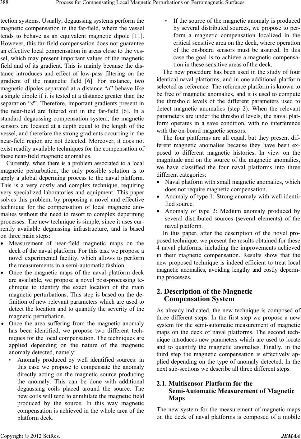

Process for Compensating Local Magnetic Perturbations on Ferromagnetic Surfaces
388
tection systems. Usually, degaussing systems perform the
magnetic compensation in the far-field, where the vessel
tends to behave as an equivalent magnetic dipole [11].
However, this far-field compensation does not guarantee
an effective local compensation in areas close to the ves-
sel, which may present important values of the magnetic
field and of its gradient. This is mainly because the dis-
tance introduces and effect of low-pass filtering on the
gradient of the magnetic field [6]. For instance, two
magnetic dipoles separated at a distance “d” behave like
a single dipole if it is tested at a distance greater than the
separation “d”. Therefore, important gradients present in
the near-field are filtered out in the far-field [6]. In a
standard degaussing compensation system, the magnetic
sensors are located at a depth equal to the length of the
vessel, and therefore the strong gradients occurring in the
near-field region are not detected. Moreover, it does not
exist readily available techniques for the compensation of
these near-field magnetic anomalies.
Currently, when there is a problem associated to a local
magnetic perturbation, the only possible solution is to
apply a global deperming process to the naval platform.
This is a very costly and complex technique, requiring
very specialized laboratories and equipment. This paper
solves this problem, by proposing a novel and effective
technique for the compensation of local magnetic ano-
malies without the need to resort to complex deperming
processes. The new technique is simple, since it uses cur-
rently available degaussing infrastructure, and is based
on three main steps:
 Measurement of near-field magnetic maps on the
deck of the naval platform. For this task we propose a
novel experimental facility, which allows to perform
the measurements in a semi-automatic fashion.
 Once the magnetic maps of the naval platform deck
are available, we propose a novel post-processing te-
chnique to identify the exact location of the main
magnetic perturbations. This step is based on the de-
finition of new relevant parameters which are used to
detect the location and to quantify the severity of the
magnetic perturbation.
• Once the area suffering from the magnetic anomaly
has been identified, we propose two different tech-
niques for the local compensation. The techniques are
applied depending on the nature of the magnetic
anomaly detected, namely:
• Anomaly produced by well identified sources: in
this case we propose to compensate the anomaly
directly acting on the magnetic source producing
the anomaly. This can be done with additional
degaussing coils placed around the source. The
new coils will tend to annihilate the magnetic field
produced by the source. In this way magnetic
compensation is achieved in the whole area of the
platform deck.
• If the source of the magnetic anomaly is produced
by several distributed sources, we propose to per-
form a magnetic compensation localized in the
critical sensitive area on the deck, where operation
of the on-board sensors must be assured. In this
case the goal is to achieve a magnetic compensa-
tion in these sensitive areas of the deck.
The new procedure has been used in the study of four
identical naval platforms, and in one additional platform
selected as reference. The reference platform is known to
be free of magnetic anomalies, and it is used to compute
the threshold levels of the different parameters used to
detect magnetic anomalies (step 2). When the relevant
parameters are under the threshold levels, the naval plat-
form operates in a save condition, with no interference
with the on-board magnetic sensors.
The four platforms are all equal, but they present dif-
ferent magnetic anomalies because they have been ex-
posed to different magnetic histories. In view on the
magnitude and on the source of the magnetic anomalies,
we have classified the four naval platforms into three
different categories:
 Naval platform with small magnetic anomalies, which
does not require magnetic compensation.
 Anomaly of type 1: Strong anomaly with well identi-
fied source.
 Anomaly of type 2: Medium anomaly produced by
several distributed sources (several elements) of the
naval platform.
In this paper, after the description of the novel pro-
posed technique, we present the results obtained for these
4 naval platforms, including the improvements achieved
in their magnetic compensation. Results show that the
new proposed technique is indeed efficient to treat local
magnetic anomalies, avoiding lengthy and costly deperm-
ing processes.
2. Description of the Magnetic
Compensation System
As already indicated, the new technique is composed of
three different steps. In the first step we propose a new
system for the semi-automatic measurement of magnetic
maps on the deck of naval platforms. The second tech-
nique introduces new parameters which are used to locate
and to quantify the magnetic anomalies. Finally, in the
third step the magnetic compensation is effectively ap-
plied depending on the type of anomaly detected. In the
next sub-sections we describe all three different steps.
2.1. Multisensor Platform for the
Semi-Automatic Measurement of Magnetic
Maps
The new system for the measurement of magnetic maps
on the deck of naval platforms is composed of a mobile

Process for Compensating Local Magnetic Perturbations on Ferromagnetic Surfaces 389
trolley made from non-magnetic material, containing three
magnetic sensors and several electronic equipments, as
shown in Figure 1.
The magnetic field is captured with full tri-axial mag-
netic sensors, and a two-axis tilt-meter is used to measure
the pitch and roll associated to each measured point. The
pitch and roll information is used to compensate for the
natural oscillations in the deck during the measurement
of the magnetic field at each point of the deck by the
magnetic sensors. The presence of these oscillations is
due to the natural movement of the naval platform and to
the roughness of the deck surface.
For the measurement of the magnetic map an origin is
selected on the deck. Starting from the origin, the trolley
moves by columns capturing the magnetic field in a mesh
of points. The distance of the points in the deck to form
the rows of the mesh is adjusted with a digital encoder.
The encoder is fixed to the axis of one wheel in the trol-
ley, and gives the angle of rotation encoded in binary
form. With this information and with the radius of the
wheel, it is possible to compute the distance between two
consecutive points in each row of the mapping system.
All these data is captured by a sampling card connected
to a computer through a USB port. The computer has
specific software, developed in LabView, for the storage
and processing of the received information. The graphic
interface of the software is shown in Figure 2. The
whole system is completed with batteries for autonomous
operation during two hours, and can be seen in Figure 1.
Before measurements are taken, the system needs to be
calibrated in distance. This is done by selecting a given
distance on the deck. This information is passed to the
graphic interface of Figure 2, and then the trolley is
made to cover the specified distance. The calibration
process measures the total number of pulses of the digital
encoder in the specified distance. With this information it
computes the number of pulses of the digital encoder per
HEIGHT POSITION
44-115cm
PITCH & ROLL
SENSOR
DIGITAL
ENCODER
EXTERNAL AD
Q
UISITION BOARD
JUNTION BOX
BATTERIES
CRADLE
55×100×31 cm
Figure 1. Mobile trolley with magnetic sensors and other
electronic equipment used for the measurement of magnetic
maps on the deck of naval platforms.
Figure 2. Graphic interface of the software developed for
capturing and processing of the information.
unit length. Once the system is calibrated it is possible to
encoder in the specified distance. With this information it
computes the number of pulses of the digital encoder per
adjust the number of sampling points per unit length,
therefore effectively selecting the mesh density.
During the measurement procedure, the signals ob-
tained by the different sensors (magnetic sensors, digital
encoder and tilt-meter) are captured by the sampling card
and are displayed in the graphic interface (Figure 2). The
system allows capturing simultaneously three columns of
the mesh, since the trolley is provided with three equally
spaced magnetic sensors, as shown in Figure 1. In this
way the measurement time is consequently reduced by
three, until the whole mesh is covered with the system.
In a practical situation, the raw data measured by the
system need to be transformed before it can be used for
the detection of magnetic anomalies. The first transfor-
mation is needed to correct the pitch and roll of the naval
platform at each sample point. With the information pro-
vided by the tilt-meter, the magnetic field measured at
each point is corrected with the following matrix trans-
formation:







0
0
0
0
0
0
,,
,,
,,
cossinsinsincos, ,
0cos sin,,
sinsincoscoscos, ,
x
y
z
x
y
z
Bijz
Bijz
Bijz
Bijz
Bijz
Bijz


 





 











 


(1)
where B'x(i,j,z0), B'y(i,j,z0) and B'z(i,j,z0) are the measured
components of the magnetic field at point (i,j) of the
mesh, taken at a fixed height z0 above the deck surface.
The angles α and β correspond to the measured roll and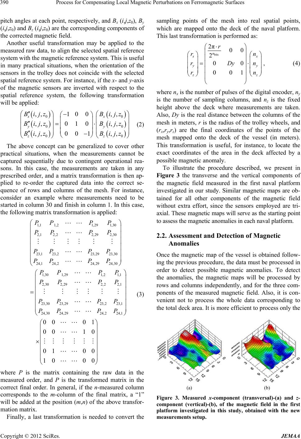

Process for Compensating Local Magnetic Perturbations on Ferromagnetic Surfaces
390
pitch angles at each point, respectively, and Bx (i,j,z0), By
(i,j,z0) and Bz (i,j,z0) are the corresponding components of
the corrected magnetic field.
Another useful transformation may be applied to the
measured raw data, to align the selected spatial reference
system with the magnetic reference system. This is useful
in many practical situations, when the orientation of the
sensors in the trolley does not coincide with the selected
spatial reference system. For instance, if the x- and y-axis
of the magnetic sensors are inverted with respect to the
spatial reference system, the following transformation
will be applied:






0
0
0
,,1 00,,
,,0 1 0,,
,,0 01,,
x
y
z
Bijz Bijz
BijzBijz
Bi jzBi jz
   

 

 
 


 
 

 

0
0
0
x
y
z

















(2)
The above concept can be generalized to cover other
practical situations, when the measurements cannot be
captured sequentially due to contingent operational rea-
sons. In this case, the measurements are taken in any
prescribed order, and a matrix transformation is then ap-
plied to re-order the captured data into the correct se-
quence of rows and columns of the mesh. For instance,
consider an example where measurements need to be
started in column 30 and finish in column 1. In this case,
the following matrix transformation is applied:
1,11,21,29 1,30
2,1 2,22,292,30
23,1 23,223,2923,30
24,124,224,2924,30
1,301,291,2 1,1
2,30 2,292,2 2,1
23,30 23,2923,2 23,1
24,30 24,2924,2
PPP P
PPP P
PPP P
PPP P
PP PP
PP PP
PP PP
PP P











 






 24,1
00 01
00 10
01 00
10 00
P


















 


(3)
where P is the matrix containing the raw data in the
measured order, and P is the transformed matrix in the
correct final order. In general, if the n-measured column
corresponds to the m-column of the final matrix, a “1”
will be added at the position (m,n) of the above transfor-
mation matrix.
Finally, a last transformation is needed to convert the
sampling points of the mesh into real spatial points,
which are mapped onto the deck of the naval platform.
This last transformation is performed as:
bits
2π00
2
00
001
n
x
x
y
y
z
z
r
rn
rDy
rn



 

 


 
  
 


n
, (4)
where nx is the number of pulses of the digital encoder, ny
is the number of sampling columns, and nz is the fixed
height above the deck where measurements are taken.
Also, Dy is the real distance between the columns of the
mesh in meters, r is the radius of the trolley wheels, and
(rx,ry,rz) are the final coordinates of the points of the
mesh mapped onto the deck of the vessel (in meters).
This transformation is useful, for instance, to locate the
exact coordinates of the area in the deck affected by a
possible magnetic anomaly.
To illustrate the procedure described, we present in
Figure 3 the transverse and the vertical components of
the magnetic field measured in the first naval platform
investigated in our study. Similar magnetic maps are ob-
tained for all other components of the magnetic field
without extra effort, since the sensors employed are tri-
axial. These magnetic maps will serve as the starting point
to assess the magnetic anomalies in each naval platform.
2.2. Assessment and Detection of Magnetic
Anomalies
Once the magnetic map of the vessel is obtained follow-
ing the previous procedure, the data must be processed in
order to detect possible magnetic anomalies. To detect
the anomalies, the magnetic maps will be processed by
rows and columns independently, and for the three com-
ponents of the measured magnetic field. Also, it is con-
venient not to process the whole data corresponding to
the total deck area. It is more efficient to process only the
(a) (b)
Figure 3. Measured x-component (transversal)-(a) and z-
component (vertical)-(b), of the magnetic field in the first
platform investigated in this study, obtained with the new
measurements setup.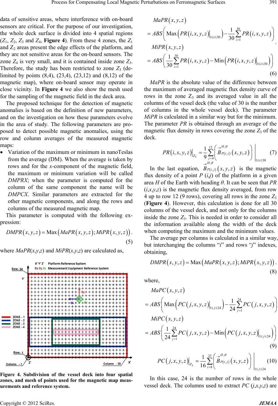

Process for Compensating Local Magnetic Perturbations on Ferromagnetic Surfaces 391
data of sensitive areas, where interference with on-board
sensors are critical. For the purpose of our investigation,
the whole deck surface is divided into 4 spatial regions
(Z1, Z2, Z3 and Z4, Figure 4). From these 4 zones, the Z1
and Z2 areas present the edge effects of the platform, and
they are not sensitive areas for the on-board sensors. The
zone Z4 is very small, and it is contained inside zone Z3.
Therefore, the study has been restricted to zone Z3 (de-
limited by points (8,4), (23,4), (23,12) and (8,12) of the
magnetic map), where on-board sensor may operate in
close vicinity. In Figure 4 we also show the mesh used
for the sampling of the magnetic field in the deck area.
The proposed technique for the detection of magnetic
anomalies is based on the definition of new parameters,
and on the investigation on how these parameters evolve
in the area of study. The following parameters are pro-
posed to detect possible magnetic anomalies, using the
row and column averages of the measured magnetic
maps:
 Variation of the maximum or minimum in nanoTeslas
from the average (DM). When the average is taken by
rows and for the x-component of the magnetic field,
the maximum or minimum variation will be called
DMPRX; when the parameter is computed for the
column of the same component the name will be
DMPCX. Similar parameters are extracted for the
other magnetic components, and along the rows and
columns of the measured magnetic map.
This parameter is computed with the following ex-
pression:
 

 
,,Max,, ;,,DMPRxyzMaPRxyzMiPRxyz

.
(5)
where MaPR(x,y,z) and MiPR(x,y,z) are calculated as,
Figure 4. Subdivision of the vessel deck into four spatial
zones, and mesh of points used for the magnetic map meas-
urements and reference system.






 

30
130 1
30
130
1
,,
1
Max, ,,, ,,
30
,,
1,,, Min,,,
30
ii
i
i
MaPRxyz
A
BSPRi x y zPRix y z
MiPRxyz
ABSPRix y zPRi x y z
 












.
(6)
MaPR is the absolute value of the difference between
the maximum of averaged magnetic flux density curve of
rows in the zone Z3 and its averaged value in all the
columns of the vessel deck (the value of 30 is the number
of columns in the whole vessel deck). The parameter
MiPR is calculated in a similar way but for the minimum.
The parameter PR is obtained through an average of the
magnetic flux density in rows covering the zone Z3 of the
deck.
  
3
,
12
,
4130
1
,,,,,
9
H
Pi j
Zji
PR ix y zBx yz








 (7)
In the last equation, is the magnetic
flux density of a point P (i,j) of the platform in a given
area H of the Earth with heading θ. It can be seen that PR
(i,x,y,z) is the magnetic flux density averaged, from row
4 up to row 12 (9 rows), covering all rows in the zone Z3
(Figure 4). However, this calculation is done for all 30
columns of the vessel deck, and not only for the columns
inside the zone Z3. This is needed in order to consider all
the information available along the width of the deck
when computing the maximum and the minimum values.


,
,,,
H
Pi j
Bxyz



The average per columns is calculated in a similar way,
but interchanging the columns “i” and rows “j” indexes,
obtaining,






,,Max,, ;,,DMPRxyzMaPRxyzMiPRxy z.
(8)
where,






 

24
124 1
24
124
1
,,
1
Max, ,,, ,,
24
,,
1,,, Min,,,
24
jj
j
j
MaPCxy z
A
BSPCj x y zPCj x y z
MiPCx y z
ABSPCj x y zPCj x y z
 












(9)
  
3
,
23
,
8124
1
,,,,,
16
H
Pi j
Zij
PC jxyzBxyz






(10)
In this case, 24 is the number of rows in the whole
vessel deck. The columns used to extract PC (j,x,y,z) are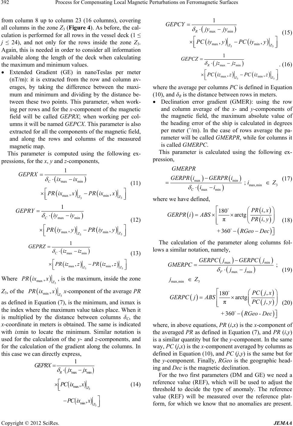

Process for Compensating Local Magnetic Perturbations on Ferromagnetic Surfaces
392
from column 8 up to column 23 (16 columns), covering
all columns in the zone Z3 (Figure 4). As before, the cal-
culation is performed for all rows in the vessel deck (1 ≤
j ≤ 24), and not only for the rows inside the zone Z3.
Again, this is needed in order to consider all information
available along the length of the deck when calculating
the maximum and minimum values.
 Extended Gradient (GE) in nanoTeslas per meter
(nT/m): it is extracted from the row and column av-
erages, by taking the difference between the maxi-
mum and minimum and dividing by the distance be-
tween these two points. This parameter, when work-
ing per rows and for the x-component of the magnetic
field will be called GEPRX; when working per col-
umns it will be named GEPCX. This parameter is also
extracted for all the components of the magnetic field,
and along the rows and columns of the measured
magnetic map.
This parameter is computed using the following ex-
pressions, for the x, y and z-components,

 
3 3
max min
max min
1
,,
C
Z Z
GEPRX ix ix
PR ixxPR ixx





 
(11)

 
3 3
max min
max min
1
,,
C
Z Z
GEPRY iyiy
PR iyyPR iyy






(12)

 
3 3
max min
max min
1
,,
C
Z Z
GEPRZ iz iz
PR izzPRizz






(13)
Where

3
max ,
Z
PR ixx, is the maximum, inside the zone
Z3, of the

3
min ,
Z
PR ixxx-component of the average PR
as defined in Equation (7), is the minimum, and ixmax is
the index where the maximum value takes place. When it
is multiplied by the distance between columns δC, the
x-coordinate in meters is obtained. The same is indicated
with ixmin to locate the minimum. Similar notation is
used for the calculation of the y- and z-components, and
for the calculation of the gradient along the columns. In
this case we can directly express,



3
3
max min
max
min
1
,
,
R
Z
Z
GEPRX jxjx
PC ixx
PC ixx








(14)



3
3
max min
max min
1
,,
R
Z Z
GEPCY jy jy
PC iyyPC iyy









(15)

 
3 3
max min
max min
1
,,
R
Z Z
GEPCZ jz jz
PC izzPCizz









. (16)
where the average per columns PC is defined in Equation
(10), and δR is the distance between rows in meters.
 Declination error gradient (GMER): using the row
and column average of the x- and y-components of
the magnetic field, the maximum absolute value of
the heading error of the ship is calculated in degrees
per meter (˚/m). In the case of rows average the pa-
rameter will be called GMERPR, while for columns it
is called GMERPC.
This parameter is calculated using the following ex-
pression,
 

max min
max,min 3
max min
;
C
GMERPR
GERPR iGERPR iiZ
ii 



(17)
where we have defined,
 


,
180 arctg
π,
360
PRi x
GERPRiABS PRi y
+ RGeo Dec

 








(18)
The calculation of the parameter along columns fol-
lows a similar notation, namely,





max min
max min
max,min 3
;
F
GERPC jGERPC j
GMERPC jj
jZ




(19)
 


,
180 arctg
π,
360
PCj x
GERPCjABS PCj y
+ RGeo - Dec










(20)
where, in above equations, PR (i,x) is the x-component of
the averaged PR as defined in Equation (7), and PR (i,y)
is a similar quantity but for the y-component. In the same
way, PC (j,x) is the x-component averaged by columns as
defined in Equation (10), and PC (j,y) is the same but for
the y-component. Finally, RGeo is the geographic head-
ing and Dec is the magnetic declination.
For the two first parameters (DM and GE) we need a
reference value (REF), which will be used to adjust the
threshold to decide the type of anomaly. The reference
value (REF) will be measured over the reference plat-
form, for which we know that no anomalies are present.

Process for Compensating Local Magnetic Perturbations on Ferromagnetic Surfaces 393
For the GMER parameter there is not a reference value,
since it measures the real heading error of the ship. The
value of DM referred to REF will classify the anomaly as
type 2 when it is in the range between 110% and 200%,
and of type 1 when it is above 200%. When this value is
below 110%, the anomaly will be considered as not sig-
nificant. For the GE parameter, again referred to the REF
value, differences below 150% are not important. In the
range between 150% and 250% will be classified as a
type 2 anomaly, and when it is above 250% the anomaly
is considered to be of type 1.
We have observed that the parameters GE and DM
using the rows or columns average have similar behavior.
However in the case of GMER there exists an important
difference when working by rows or by columns. This is
because the GMER parameter measures real errors of
heading, and they can be very different in the two main
directions of the vessel. When GMERPR is between 0˚/m
and 13˚/m it is not considered as magnetic anomaly. A
type 2 anomaly has a value between 13˚/m and 18˚/m.
Values above 18˚/m indicate that a type 1 anomaly is
present. When working by columns, the parameter
GMERPC need to be more restrictive, since along this
direction there are no symmetries in the ferromagnetic
materials of the vessel. As a consequence the parameter
is naturally lower, and a lower threshold will indicate the
beginning of a magnetic anomaly. In this case, values of
GMERPC below 7˚/m show no anomaly; between 7˚/m
and 10˚/m an anomaly of type 2 and above 10˚/m reveals
an anomaly of type 1. In Table 1 we collect the classi-
fication of the different types of anomaly, depending on
the values of the different parameters defined in this
work. The thresholds have been obtained from experi-
mentation, taking into consideration the expertise and
recommendations of renowned operators in vessels decks.
In principle they can be applied to other vessels and plat-
form types.
2.3. Anomaly Compensation
Once a given magnetic anomaly is detected using the
new parameters defined in the previous section, two
methods are suggested to compensate for the magnetic
Table 1. Classification of the different types of anomalies as
a function of the different parameters defined in this work.
ANOMALY
Parameter/
Reference NO Type 2 Type 1
DM/REF <1.1 1.1 ≤ DM/REF < 2 ≥2
GE/REF <1.5 1.5 ≤ GE/REF < 2.5 ≥2.5
GMERPR 0< GMERPR < 13 13 ≤ GMERPR < 18 GMERPR ≥ 18
GMERPC 0 < GMERPC < 7 7 ≤ GMERPC < 10 GMERPC ≥ 10
anomaly. In the first case (strong anomaly or type 1) the
magnetic source is known and it has been identified. In
this situation we propose to use additional coils around
the source, to compensate the produced magnetic field
directly on the source. The situation of the coils will de-
pend on the orientation of the magnetization created by
the source. The second situation is produced by a type 2
anomaly, which is not localized into a specific magnetic
source, but rather is due to several distributed elements.
In this case we propose to focus the compensation to a
given area of the deck, where the sensitive magnetic
sensors must operate. This problem will be treated using
vertical coils (horizontal plane), with maximum dimen-
sions similar to the distance to the area where the com-
pensation is desired.
For both techniques, the number of coils will depend
on the surface to compensate. Also, the compensation of
the distributed anomaly (type 2) needs more coils than
for anomalies of type 1. The value of the currents and the
number of turns in each coil, in both cases, will be cal-
culated using the Genetic Algorithm (GA) method des-
cribed in [1].
3. Results
The techniques described above have been applied to
five naval platforms, one of them taken as reference. As
a result of this study we have found a magnetic anomaly
in two of them, one of type 1 and the other of type 2.
As we described in Section 2.2 the detection of the
anomalies is based on the study of several parameters. In
particular, we have studied DM, and GE for the x-, y- and
z-components of the magnetic field, evaluated per row
and column averages. In addition, the parameter GMER
was also evaluated per rows and columns to assess the
declination error gradient in both navigation directions of
the vessel. In this experiment, the anomalies detected
presented strong transversal magnetic components pro-
duced by one or several transversal sources. These mag-
netic anomalies are detected in the x-component of the
above mentioned parameters. Therefore, we only present
the results obtained for the parameters DMPRX, GEPRX,
GMERPR and GMERPC.
Figure 5 shows the average of the x-component of the
magnetic field computed per rows, along the columns
defined inside the zone Z3 of Figure 4, and for the five
naval platforms investigated.
From this average we can easily compute the parame-
ters DMPRX (nT) and GEPRX (nT/m) for all five naval
platforms, as shown in Table 2. From the results we ob-
serve that the first naval platform (P1) presents very high
values of the DMPRX parameter, indicating a strong
anomaly produced by a transversal source. Also the pa-
rameter GEPRX is high, confirming the presence of an

Process for Compensating Local Magnetic Perturbations on Ferromagnetic Surfaces
394
Points in meters (port to starboard)
Figure 5. Results obtained for the average of the x-component of the magnetic field computed per rows, for all naval plat-
forms studied. Variation along columns inside zone Z3.
Table 2. Numerical values obtained for DMPRX and
GEPRX for all five naval platforms.
PLATFORM DMPRX
(nT) DMPRX/REF GEPRX (nT/m) GEPRX/REF
PREF 4.642 - 1.245 -
P1 18.479 3.98 4.827 3.88
P2 1.312 0.28 1.480 1.19
P3 4.216 0.91 855 0.69
P4 5.207 1.21 2.467 1.98
important anomaly in this platform.
According to the thresholds established in the previous
section, we can easily verify that platform (P1) is classi-
fied as severe anomaly of type 1, while platform (P4) as
anomaly of type 2. Platforms (P2) and (P3) maintain the
DMPRX and GEPRX values below the thresholds (1.1 ×
4.642 = 5.106 and 1.5 × 1.245 = 1.868, respectively), and
they are thus considered to be free of anomalies.
Once the previous parameters are studied for all three
components of the magnetic field, we proceed to the
calculation of the heading errors along both rows and
columns (GMERPR and GMERPC). These two parame-
ters are extracted from the declination of the horizontal
components of the magnetic field (angles between the x-
and y-components of the magnetic field referred to the
two main directions of the platform). The variation of the
declination along the two main directions inside the zone
Z3 in all five platforms is shown in Figures 6 and 7.
From these Graphics we can extract the final GMERPR
and GMERPC parameters for the five platforms studied,
as shown in Table 3.
From the obtained results we can conclude that the
heading errors are higher in platform (P1) than in the
other platforms measured, confirming the strong anomaly
present in this platform. According to the thresholds
given in the previous section, platform (P1) has again an
anomaly of type 1 and platform (P4) has and anomaly of
type 2. These values confirm that the other platforms do
not have any magnetic anomaly, since these parameters
remain below the specified thresholds.
Once the anomalies have been detected, we propose
two different techniques for compensation, depending on
the type of the anomaly detected. In the case of type 1
anomaly, present in platform (P1), we propose a com-
pensation acting directly on the magnetic source respon-
sible for the anomaly. For this platform (P1), the critical
area is delimited by rows 2 - 10 and by columns 9 - 21 of
the magnetic map. This can be observed in Figure 8,
where we show the measured x-component of the mag-
netic field from port to starboard.
From the measured results we can observe both high
values and fast variations of this component of the mag-
netic field.
The compensation in this case is performed with two
vertical coils (that we call MBr and MEr) placed under the
deck (at a depth of three meters), around the identified

Process for Compensating Local Magnetic Perturbations on Ferromagnetic Surfaces 395
Points in meters (port to starboard)
Figure 6. Absolute declination of the horizontal magnetic field along columns inside zone Z3.
Points in meters (bow-stern)
Figure 7. Absolute declination of the horizontal magnetic field along rows inside zone Z3.
sources, as shown in Figure 9 (yellow color). Each coil
is used to compensate one of the identified magnetic
sources.
Using the optimization technique presented in [1], we
can compute the values of the currents and the number of
turns in each coil needed to reduce the magnetic field
created by the identified sources. In this case, the opti-
mization algorithm converged for a current of −2000
Amp/Turn in coil MBr and 7000 Amp/Turn for coil MEr.
In Figure 10 we show the x-component of the magnetic
field obtained after compensation, indicating a reduction
of the magnetic field in about 71% with respect to the
initial values shown in Figure 8.
The compensation of the type 2 anomaly present in plat-
form (P4) is more complex, since a strong source causing
the magnetic anomaly cannot be identified. This mag-
netic anomaly is probably due to the interaction of sev-
eral weak sources distributed in several areas of the plat-
form. Figure 11 shows the measured x-component of the
magnetic field in platform (P4) before compensation.
In this case, compensation is performed in the area
where the sensitive sensors must operate (in our case
between columns 12 and 25). For this purpose a total of
fifteen coils have been used, distributed in the relevant area

Process for Compensating Local Magnetic Perturbations on Ferromagnetic Surfaces
396
of the deck. In Figure 12 we show a drawing of the deck,
indicating in red the zone of the magnetic anomaly. The
numbers in blue show the location of the fifteen coils
used for compensation.
Using again the method described in [1], the currents
to each coil and the number of turns are optimized. This
information is collected in Table 4.
To show the effectiveness of the proposed approach,
we present in Figure 13 the measured magnetic field
Table 3. Final values obtained for GMERPR and GMERPC.
Anomaly
Platform GMERPR
NO
GMERPF
< 13
TYPE 2
13 <
GMERPF <
18
TYPE 1
(GMERPF
> 18)
PREF 11
P1 20 X
P2 10 X
P3 6 X
P4 15 X
Anomaly
Platform GMERPC
NO
GMERPC
< 7
TYPE 2
7<
GMERPC
< 10
TYPE 1
(GMERPC
> 10)
PREF 4
P1 12 X
P2 6 X
P3 4 X
P4 9 X
obtained after compensation. Results demonstrate that a
gradient reduction of 30% can be achieved, which is suf-
ficient for most practical applications.
In Table 5 values for parameters DMPRX, GEPRX,
GMERPR and GMERPC before and after compensation are
shown.
It can be observed from above table that substantial
reduction in the anomaly parameters are obtained after
applying the compensation techniques. In particular, the
new values obtained are below the specified thresholds
given in Table 1, indicating that the platforms are now
free of anomalies, thus fully validating the approach pre-
sented in this paper.
4. Conclusions
Sometimes naval platforms present local magnetic
anomalies that cannot be compensated by standard de-
gaussing systems. The authors propose in this paper a
novel method to detect, quantify and correct these local
perturbations. This will avoid the application of complex
and expensive deperming processes.
The detected anomalies have been classified in two
types depending on the number of sources and the mag-
netization strength. The anomaly of type 1 is a strong
anomaly with well identified source. The anomaly of
type 2 is a medium anomaly produced by several weak
sources (several elements) of the naval platform. Results
show that the compensation technique is more effective
and easy to introduce in the type 1 anomaly.
The described method has been applied to a real situa-
tion composed of five naval platforms. The technique has
proved its effectiveness in anomaly detection, quantifica-
tion and subsequent compensation of undesired local
magnetic anomalies, present in the investigated platforms.
Magnetic Map (z-component)
Points in meters (bow-stern)
Figure 8. Measured x-component of the magnetic field in platform (P1) before compensation, from port to starboard.

Process for Compensating Local Magnetic Perturbations on Ferromagnetic Surfaces 397
Transversal Coils
Vertical Coils
MBr & MEr
Magnetic
Sources
Column -1Column -30
Row -24
Row -1
ZONE 1
ZONE 2
ZONE 3
ZONE 4
Figure 9. Surface of the deck showing the mesh. The location of the additional coils used in the compensation of platform (P1)
is marked with yellow lines.
Vertical Coils Compensation (z-component)
Points in meters (port to starboard)
Figure 10. Measured x-component of the magnetic field for rows 2 - 10 from port to starboard after compensation with coils
MBr and MEr.
Magnetic Map (z-component)
Points in meters (port to starboard)
Figure 11. Measured x-component of the magnetic field in platform (P4) before compensation, from port to starboard.

Process for Compensating Local Magnetic Perturbations on Ferromagnetic Surfaces
398
Table 4. Optimized values of the currents to each coil
needed for compensation of platform (P4).
Coil Amp/Turn CoilAmp/Turn Coil Amp/Turn
1 136 6 138 11 67
2 128 7 334 12 450
3 48 8 475 13 433
4 274 9 97 14 292
5 99 10 152 15 142
Figure 12. Zone of the magnetic anomaly (in red), and dis-
tribution of the coils for compensation.
Vertical Coils Compensation (z-component)
Points in meters (port to starboard)
Figure 13. Measured x-component of the magnetic field from port to starboard after compensation with 15 degaussing coils.
Table 5. Values obtained for DMPRX, GEPRX, GMERPR
and GMERPC before and after compensation for Platforms
P1 and P4.
Platform DMPRX/REF GEPRX/REF GMERPR/PC ˚/m
P1 Before 3.98 3.88 20/12
P1 After 0.57 1.05 5/6
P4 Before 1.21 1.98 15/9
P4 After 0,82 1.11 4/4
5. Acknowledgements
This work was supported under Spanish National project
TEC2010-21520-C04-04 and European Feder Fundings.
REFERENCES
[1] A. V. Madrid and A. Á. Melcón, “Using Genetic Algo-
rithms for Compensating the Local Magnetic Perturbation
of a Ship in the Earth´s Magnetic Field,” Microwave and
Optical Technology Letters, Vol. 47, No. 3, 2005, pp. 281-
287.
[2] F. L. Dorze, J. P. Bongiraud, J. L. Coulomb, P. Labie and
X. Brunote, “Modeling of Degaussing Coils Effects in
Ships by the Method of Reduced Scalar Potencial Jump,”
IEEE Transaction on Magnetics, Vol. 34, No. 5, 1998, pp.
2477-2480.
[3] X. Brunotte and G. Meunier, “Line Element for Efficient
Computation of the Magnetic Field Created by Thin Iron
Plates,” IEEE Transaction on Magnetics, Vol. 26, No. 5,
1990, pp. 2196-2198.
[4] X. Brunotte, G. Meunier and J. P. Bongiraud, “Ship
Magnetizations Modelling by the Finite Element Me-
thod,” IEEE Transaction on Magnetics, Vol. 29, No. 2,
1993, pp. 1970-1975.
[5] D. Rogers, P. J. Leonard and H. C. Lai, “Surface Ele-
ments for Modelling 3D Fields around Thin Iron Sheets,”
IEEE Transaction on Magnetics, Vol. 29, No. 25, 1993,
pp. 1483-1486.
[6] J. J. Holmes, “Application of Models in the Design of
Underwater Electromagnetic Signature Reduction Sys-
tems,” Naval Engineers Journal, Vol. 119, No. 4, 2007,
pp. 19-29. doi:10.1111/j.1559-3584.2007.00083.x
[7] D. S. Weile and E. Michielssen, “Genetic Algorithm Op-
timization Applied to Electromagnetics: A Review,”
IEEE Transaction on Antennas and Propagation, Vol. 45,
No. 3, 1997, pp. 343-353.
[8] D. E. Goldberg, “Genetic Algorithm in Search, Optimiza-
tion and Machine Learning,” Addison-Wesley Publishing
Company, Boston, 1989.

Process for Compensating Local Magnetic Perturbations on Ferromagnetic Surfaces 399
[9] H. Liu and Z. Ma, “Optimization of Warship Degaussing
System Based on Poly-Population Particle Swarm Algo-
rithm,” International Conference on Mechatronic and Au-
tomation, ICMA, Harbin, 5-8 August 2007, pp. 3133-
3137.
[10] W. C. Potts, “The Magnetic Field of a Ship and Its Neu-
tralization by Coil Degaussing,” General Journal of the
Institution of Electrical Engineers—Part I, Vol. 93, No.
71, 1946, pp. 488-499.
[11] Y.-T. Yang, Z.-Y. Shi, J.-G. Lu and Z.-Z. Guan, “A
Magnetic Disturbance Compensation Method Based on
Magnetic Dipole Magnetic Field Distributing Theory,”
Journal of China Ordenance, Vol. 5, No. 3, 2009, pp.
185-191.
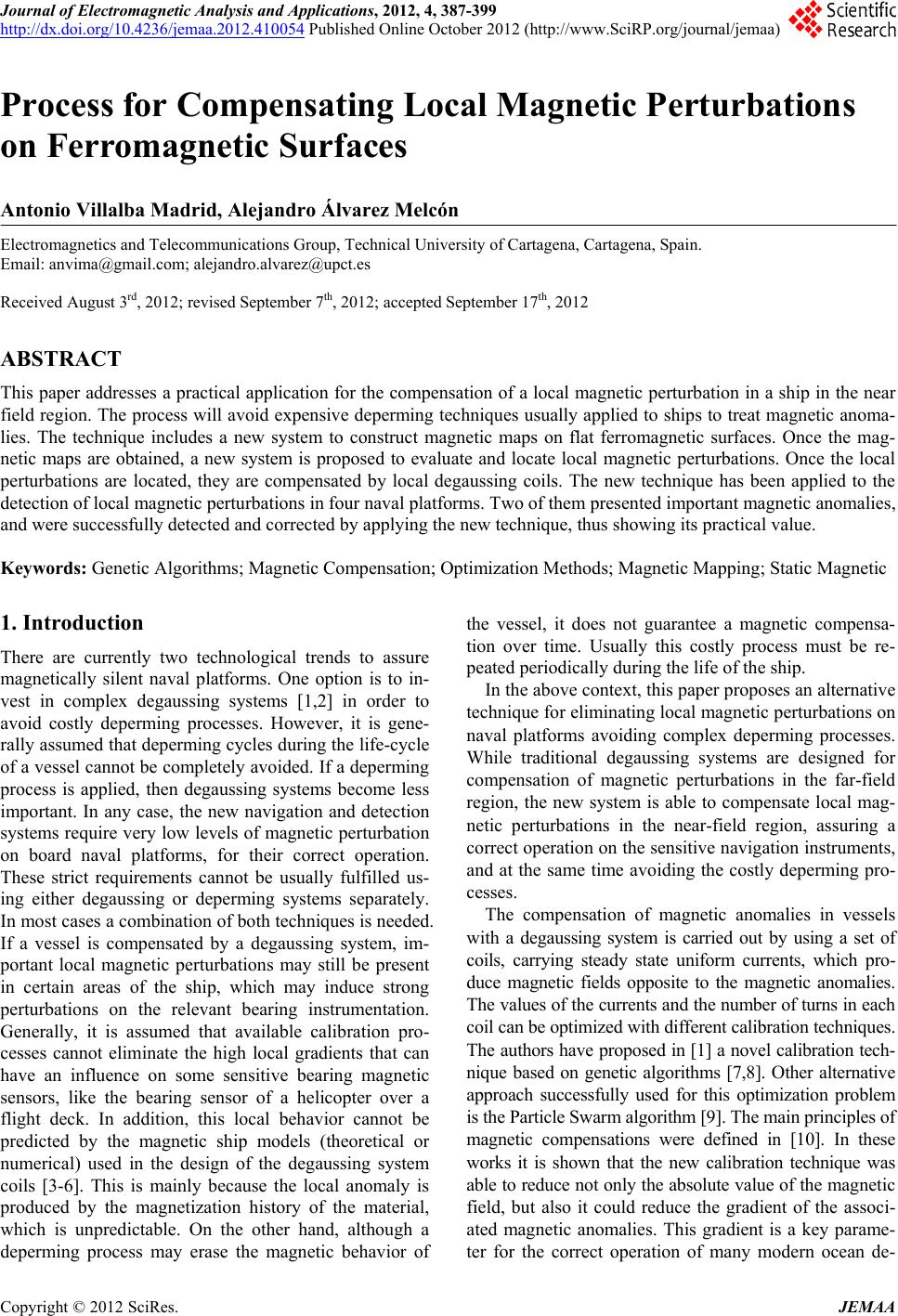