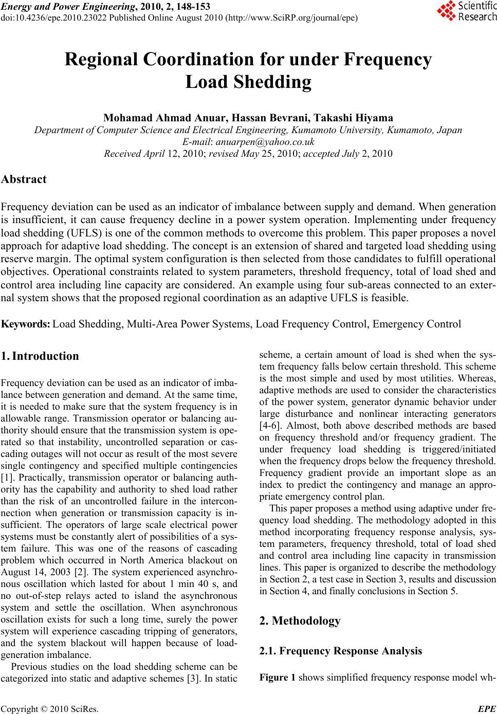Energy and Power Engineering, 2010, 2, 148-153
doi:10.4236/epe.2010.23022 Published Online August 2010 (http://www.SciRP.org/journal/epe)
Regional Coordination for under Frequency
Load Shedding
Mohamad Ahmad Anuar, Hassan Bevrani, Takashi Hiyama
Department of Computer Science and Electrical Engineering, Kumamoto University, Kumamoto, Japan
Received April 12, 2010; revised May 25, 2010; accepted July 2, 2010
Abstract
Frequency deviation can be used as an indicator of imbalance between supply and demand. When generation
is insufficient, it can cause frequency decline in a power system operation. Implementing under frequency
load shedding (UFLS) is one of the common methods to overcome this problem. This paper proposes a novel
approach for adaptive load shedding. The concept is an extension of shared and targeted load shedding using
reserve margin. The optimal system configuration is then selected from those candidates to fulfill operational
objectives. Operational constraints related to system parameters, threshold frequency, total of load shed and
control area including line capacity are considered. An example using four sub-areas connected to an exter-
nal system shows that the proposed regional coordination as an adaptive UFLS is feasible.
Keywords: Load Shedding, Multi-Area Power Systems, Load Frequency Control, Emergency Control
1. Introduction
Frequency deviation can be used as an indicator of imba-
lance between generation and demand. At the same time,
it is needed to make sure that the system frequency is in
allowable range. Transmission operator or balancing au-
thority should ensure that the transmission system is ope-
rated so that instability, uncontrolled separation or cas-
cading outages will not occur as result of the most severe
single contingency and specified multiple contingencies
[1]. Practically, transmission operator or balancing auth-
ority has the capability and authority to shed load rather
than the risk of an uncontrolled failure in the intercon-
nection when generation or transmission capacity is in-
sufficient. The operators of large scale electrical power
systems must be constantly alert of possibilities of a sys-
tem failure. This was one of the reasons of cascading
problem which occurred in North America blackout on
August 14, 2003 [2]. The system experienced asynchro-
nous oscillation which lasted for about 1 min 40 s, and
no out-of-step relays acted to island the asynchronous
system and settle the oscillation. When asynchronous
oscillation exists for such a long time, surely the power
system will experience cascading tripping of generators,
and the system blackout will happen because of load-
generation imbalance.
Previous studies on the load shedding scheme can be
categorized into static and adaptive schemes [3]. In static
scheme, a certain amount of load is shed when the sys-
tem frequency falls below certain threshold. This scheme
is the most simple and used by most utilities. Whereas,
adaptive methods are used to consider the characteristics
of the power system, generator dynamic behavior under
large disturbance and nonlinear interacting generators
[4-6]. Almost, both above described methods are based
on frequency threshold and/or frequency gradient. The
under frequency load shedding is triggered/initiated
when the frequency drops below the frequency threshold.
Frequency gradient provide an important slope as an
index to predict the contingency and manage an appro-
priate emergency control plan.
This paper proposes a method using adaptive under fre-
quency load shedding. The methodology adopted in this
method incorporating frequency response analysis, sys-
tem parameters, frequency threshold, total of load shed
and control area including line capacity in transmission
lines. This paper is organized to describe the methodology
in Section 2, a test case in Section 3, results and discussion
in Section 4, and finally conclusions in Section 5.
2. Methodology
2.1. Frequency Response Analysis
Figure 1 shows simplified frequency response model wh-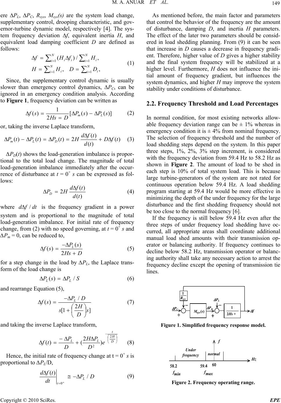

M. A. ANUAR ET AL.
149
ere ∆PL, ∆PC, Rsys, Msys(s) are the system load change,
supplementary control, drooping characteristic, and gov-
ernor-turbine dynamic model, respectively [4]. The sys-
tem frequency deviation ∆f, equivalent inertia H, and
equivalent load damping coefficient D are defined as
follows:






N
ii
N
ii
N
ii
N
iii
DD HH
HfHf
11
11
,,
,/)( (1)
Since, the supplementary control dynamic is usually
slower than emergency control dynamics, ∆PC, can be
ignored in an emergency condition analysis. According
to Figure 1, frequency deviation can be written as
)]()([
2
1
)( sPsP
D
H
s
sf Lm 

 (2)
or, taking the inverse Laplace transform,
)(
)(
)(
2)()()( tfD
td
tfd
HtPtPtPDLm 

 (3)
∆PD(t) shows the load-generation imbalance is propor-
tional to the total load change. The magnitude of total
load-generation imbalance immediately after the occur-
rence of disturbance at t = 0+ s can be expressed as fol-
lows:
)(
)(
2td
tfd
HPD

 (4)
where dtfd / is the frequency gradient in a power
system and is proportional to the magnitude of total
load-generation imbalance. For initial rate of frequency
change, from (2) with no speed governing, at t = 0+ s and
∆Pm = 0, can be reduced to,
DHs
sP
sf L


 2
)(
)( (5)
for a step change in the load by ∆PL, the Laplace trans-
form of the load change is
SPsP LL /)(  (6)
and rearrange Equation (5),
]
2
1[
/
)(
s
D
H
s
DP
sf L








 (7)
and taking the inverse Laplace transform,










 D
H
t
LL e
D
PH
D
P
tf
2
2)
2
()( (8)
Hence, the initial rate of frequency change at t = 0+ s is
proportional to ∆PL/D,
DP
dt
tfd
L
t
/
)(
0




(9)
As mentioned before, the main factor and parameters
that control the behavior of the frequency are the amount
of disturbance, damping D, and inertia H parameters.
The effect of the later two parameters should be consid-
ered in load shedding planning. From (9) it can be seen
that increase in D causes a decrease in frequency gradi-
ent. Therefore, higher value of D gives a higher stability
and the final system frequency will be stabilized at a
higher level. Furthermore, H does not influence the ini-
tial amount of frequency gradient, but influences the
system dynamics, and higher H may improve the system
stability under conditions of disturbance.
2.2. Frequency Threshold and Load Percentages
In normal condition, for most existing networks allow-
able frequency deviation range can be ± 1% whereas in
emergency condition it is ± 4% from nominal frequency.
The selection of frequency threshold and the number of
load shedding steps depend on the system. In this paper
three steps, 1%, 2%, 3% step increment, is considered
with the frequency deviation from 59.4 Hz to 58.2 Hz as
shown in Figure 2. The amount of load to be shed in
each step is 10% of total system load. This is because
large turbine-generators of the system are not rated for
continuous operation below 59.4 Hz. A load shedding
program starting at 59.4 Hz would be more effective in
minimizing the depth of the under frequency for the large
disturbance and the first shedding frequency should not
be too close to the normal frequency [6].
If the frequency is still below 59.4 Hz even after the
three steps of under frequency load shedding have oc-
curred, all appropriate areas shall coordinate additional
manual load shed amounts with their transmission op-
erator or balancing authority. If frequency continues to
decline below 58.2 Hz, transmission operator or balanc-
ing authority shall take any necessary action to arrest the
frequency decline except the opening of transmission tie
lines.
 P
C
-
+
sy
s
M
(s)

P
L
+
-
2Hs +
1

f

P
m
R
s
y
s
1
Figure 1. Simplified frequency response model.


f





normal
Under
frequency
H
z
fmax
fmin
Figure 2. Frequency operating range.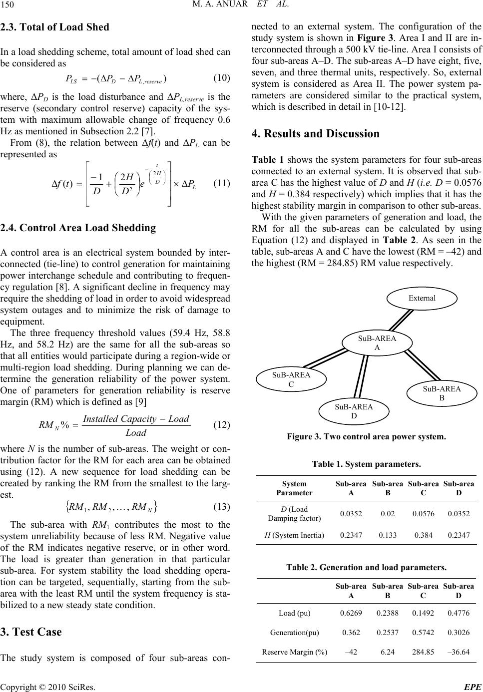

M. A. ANUAR ET AL.
150
2.3. Total of Load Shed
In a load shedding scheme, total amount of load shed can
be considered as
)(,reserveLDLS PPP  (10)
where, ΔPD is the load disturbance and ΔPL,reserve is the
reserve (secondary control reserve) capacity of the sys-
tem with maximum allowable change of frequency 0.6
Hz as mentioned in Subsection 2.2 [7].
From (8), the relation between Δf(t) and ΔPL can be
represented as
L
D
H
t
Pe
D
H
D
tf 


















 





2
2
21
)( (11)
2.4. Control Area Load Shedding
A control area is an electrical system bounded by inter-
connected (tie-line) to control generation for maintaining
power interchange schedule and contributing to frequen-
cy regulation [8]. A significant decline in frequency may
require the shedding of load in order to avoid widespread
system outages and to minimize the risk of damage to
equipment.
The three frequency threshold values (59.4 Hz, 58.8
Hz, and 58.2 Hz) are the same for all the sub-areas so
that all entities would participate during a region-wide or
multi-region load shedding. During planning we can de-
termine the generation reliability of the power system.
One of parameters for generation reliability is reserve
margin (RM) which is defined as [9]
Load
LoadCapacity Installed
RM N

% (12)
where N is the number of sub-areas. The weight or con-
tribution factor for the RM for each area can be obtained
using (12). A new sequence for load shedding can be
created by ranking the RM from the smallest to the larg-
est.

N
RMRMRM ,,, 21 (13)
The sub-area with RM1 contributes the most to the
system unreliability because of less RM. Negative value
of the RM indicates negative reserve, or in other word.
The load is greater than generation in that particular
sub-area. For system stability the load shedding opera-
tion can be targeted, sequentially, starting from the sub-
area with the least RM until the system frequency is sta-
bilized to a new steady state condition.
3. Test Case
The study system is composed of four sub-areas con-
nected to an external system. The configuration of the
study system is shown in Figure 3. Area I and II are in-
terconnected through a 500 kV tie-line. Area I consists of
four sub-areas A–D. The sub-areas A–D have eight, five,
seven, and three thermal units, respectively. So, external
system is considered as Area II. The power system pa-
rameters are considered similar to the practical system,
which is described in detail in [10-12].
4. Results and Discussion
Table 1 shows the system parameters for four sub-areas
connected to an external system. It is observed that sub-
area C has the highest value of D and H (i.e. D = 0.0576
and H = 0.384 respectively) which implies that it has the
highest stability margin in comparison to other sub-areas.
With the given parameters of generation and load, the
RM for all the sub-areas can be calculated by using
Equation (12) and displayed in Table 2. As seen in the
table, sub-areas A and C have the lowest (RM = –42) and
the highest (RM = 284.85) RM value respectively.
SuB-AREA
A
SuB-AREA
B
External
SuB-AREA
C
SuB-AREA
D
Figure 3. Two control area power system.
Table 1. System parameters.
System
Parameter
Sub-area
A
Sub-area
B
Sub-area
C
Sub-area
D
D (Load
Damping factor) 0.03520.02 0.05760.0352
H (System Inertia) 0.23470.133 0.384 0.2347
Table 2. Generation and load parameters.
Sub-area
A
Sub-area
B
Sub-area
C
Sub-area
D
Load (pu) 0.62690.2388 0.1492 0.4776
Generation(pu) 0.362 0.2537 0.5742 0.3026
Reserve Margin (%)–42 6.24 284.85 –36.64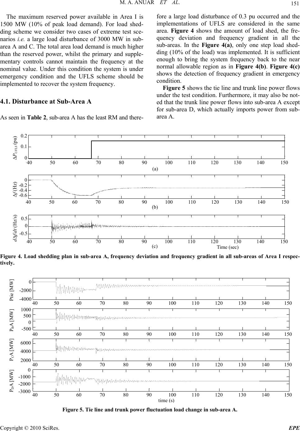

M. A. ANUAR ET AL.
151
The maximum reserved power available in Area I is
1500 MW (10% of peak load demand). For load shed-
ding scheme we consider two cases of extreme test sce-
narios i.e. a large load disturbance of 3000 MW in sub-
area A and C. The total area load demand is much higher
than the reserved power, whilst the primary and supple-
mentary controls cannot maintain the frequency at the
nominal value. Under this condition the system is under
emergency condition and the UFLS scheme should be
implemented to recover the system frequency.
4.1. Disturbance at Sub-Area A
As seen in Table 2, sub-area A has the least RM and there-
fore a large load disturbance of 0.3 pu occurred and the
implementations of UFLS are considered in the same
area. Figure 4 shows the amount of load shed, the fre-
quency deviation and frequency gradient in all the
sub-areas. In the Figure 4(a), only one step load shed-
ding (10% of the load) was implemented. It is sufficient
enough to bring the system frequency back to the near
normal allowable region as in Figure 4(b). Figure 4(c)
shows the detection of frequency gradient in emergency
condition.
Figure 5 shows the tie line and trunk line power flows
under the test condition. Furthermore, it may also be not-
ed that the trunk line power flows into sub-area A except
for sub-area D, which actually imports power from sub-
area A.
40 50 60 70 80 90100 110 120 130 140150
0
0. 1
0. 2
(a)

P
UFLS
(pu)
40 50 60 70 80 90100 110 120 130 140150
-0.6
-0.4
-0.2
0
(b)

f (Hz)
-0.5
0
0. 5
d

f/dt (Hz/s)
ΔPUFLS (pu) Δf (Hz)
dΔf/dt (Hz/s)
(a)
(b)
(c)
0
-0.2
-0.4
-0.6
0.5
0
-0.5
40 50 60 70 80 90 100 110 120 130 140 150
Time
(
sec
)
40 50 60 70 80 90 100 110 120 130 140 150
40 50 60 70 80 90 100 110 120 130 140 150
0.2
0.1
0
Figure 4. Load shedding plan in sub-area A, frequency deviation and frequency gradient in all sub-areas of Area I respec-
tively.
4
050 60 70 80 90 100 110 120 130 14015
4
050 60 70 80 90 100 110 120 130 14015
4
050 60 70 80 90 100 110 120 130 14015
4
050 60 70 80 90 100 110 120 130 14015
Ptie [MW]
40 50 60 70 80 90 100 110 120 130 140 15
0
time
(
s
)
0
-200 0
-400 0
PBA [MW]
PDA [MW] PCA [MW]
1000
500
0
-500
6000
4000
2000
0
-1000
-2000
-3000
40 50 60 70 80 90 100 110 120 130 140 15
0
40 50 60 70 80 90 100 110 120 130 140 15
0
40 50 60 70 80 90 100 110 120 130 140 15
0
Figure 5. Tie line and trunk power fluctuation load change in sub-area A.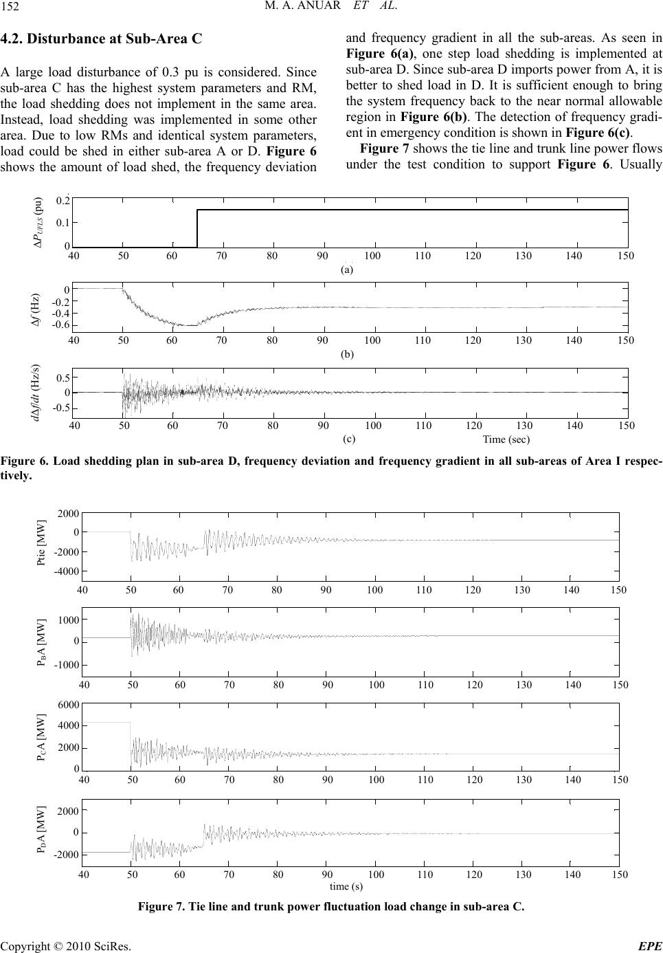

M. A. ANUAR ET AL.
152
4.2. Disturbance at Sub-Area C
A large load disturbance of 0.3 pu is considered. Since
sub-area C has the highest system parameters and RM,
the load shedding does not implement in the same area.
Instead, load shedding was implemented in some other
area. Due to low RMs and identical system parameters,
load could be shed in either sub-area A or D. Figure 6
shows the amount of load shed, the frequency deviation
and frequency gradient in all the sub-areas. As seen in
Figure 6(a), one step load shedding is implemented at
sub-area D. Since sub-area D imports power from A, it is
better to shed load in D. It is sufficient enough to bring
the system frequency back to the near normal allowable
region in Figure 6(b). The detection of frequency gradi-
ent in emergency condition is shown in Figure 6(c).
Figure 7 shows the tie line and trunk line power flows
under the test condition to support Figure 6. Usually
4
050 60 70 80 90 100 110 120 130 140 1
5
0
2
(a)
4
050 60 70 80 90 100 110 120 130 140 1
5
6
4
2
0
(b)
5
0
5
ΔP
UFLS
(pu)
Δf (Hz)
dΔf/dt (Hz/s)
0.2
0.1
0
(b)
(c)
0
-0.2
-0.4
-0.6
0.5
0
-0.5
40 50 60 70 80 90 100 110 120 130 140 150
Time
(
sec
)
(a)
40 50 60 70 80 90 100 110 120 130 140 150
40 50 60 70 80 90 100 110 120 130 140 15
0
Figure 6. Load shedding plan in sub-area D, frequency deviation and frequency gradient in all sub-areas of Area I respec-
tively.
4
050 60 70 8090100 110 120 130 140 150
4
050 60 70 8090100 110 120 130 140 150
4
050 60 70 8090100 110 120 130 140 150
4
050 60 70 8090100 110 120 130 140 150
time[s]
Ptie [MW]
time
(
s
)
2000
0
-2000
-4000
P
B
A [MW]
P
D
A [MW] P
C
A [MW]
1000
0
-1000
6000
4000
2000
0
2000
0
-2000
40 50 60 70 80 90 100 110 120 130 140 150
40 50 60 70 80 90 100 110 120 130 140 150
40 50 60 70 80 90 100 110 120 130 140 150
40 50 60 70 80 90 100 110 120 130 140 150
Figure 7. Tie line and trunk power fluctuation load change in sub-area C.

M. A. ANUAR ET AL.
153
sub-area C will transfer power to sub-area A before the
disturbance took place. But, in this case, 0.3 pu distur-
bance is manageable to load-generation imbalance (gen-
eration is greater than load) as discussed in Table 2. So,
sub-area C reduced power transfer to sub-area A after the
disturbance. Consequently sub-area A reduced power
transfer to sub-area D. Hence, Figure 7 is the evidence
of the amounts of power transfer from sub-area C to A
and sub-area A to D in a drastic reduction manner.
5. Conclusions
Regional coordination in emergency conditions is very im-
portant for power system operation and security. These
regions are interconnected to each other for improving
reliability and reducing cost. Practically, each region has
different generation and load. This condition will affect
reserve margin. The reserve margin is used to identify a
sequential load shedding. This paper shows that regional
coordination for four sub-areas connected to an external
system using adaptive under frequency load shedding is
feasible.
6. Acknowledgements
The authors would like to thank Graduate School of Sci-
ence and Technology (GSST), Kumamoto University,
Japan and MARA University of Technology (UiTM),
Malaysia for continuous support of this research.
7. References
[1] R. Baldick, B. Chowdhury, I. Dobson, Z. Dong, B. Gou,
D. Hawkins, H. Huang, M. Joung, D. Kirschen, F. X. Li,
J. Li, Z. Y. Li, C.-C. Liu, L. Mili, S. Miller, R. Podmore,
K. Schneider, K. Sun, D. Wang, Z. G. Wu, P. Zhang, W.
J. Zhang and X. P. Zhang, “Initial Review of Methods for
Cascading Failure Analysis in Electric Power Transmis-
sion Systems,” IEEE Power and Energy Society General
Meeting, Pittsburgh, 20-24 July 2008, pp. 1-8.
[2] Y. Liu and Y. Liu, “Aspects on Power System Islanding
for Preventing Widespread Blackout,” Proceeding of the
2006 IEEE International Conference on Networking,
Sensing and Control, Ft. Lauderdale, 23-25 April 2006,
pp. 1090-1095.
[3] J. J. Ford, H. Bevrani and G. Ledwich, “Adaptive Load
Shedding and Regional Protection,” International Jour-
nal of Electrical Power & Energy Systems, Vol. 31, No.
10, 2009, pp. 611-618.
[4] H. Bevrani, G. Ledwich and J. J. Ford, “On the Use of
df/dt in Power System Emergency Control,” Proceedings
of IEEE Power Systems Conferences and Exposition, Se-
attle, 15-18 March 2009, pp. 1-6.
[5] T. Tomsic, G. Verbic and F. Gubina, “Revision of the
Underfrequency Load-Shedding Scheme of the Slovenian
Power System,” Electric Power Systems Research, Vol.
77, No. 5-6, 2007, pp. 494-500.
[6] S.-J. Huang and C.-C. Huang, “Adaptive Load Shedding
Method with Time-Based Design for Isolated Power Sys-
tems,” International Journal of Electrical Power & En-
ergy Systems, Vol. 22, No. 1, 2000, pp. 51-58.
[7] H. Bevrani, “Robust Power System Frequency Control,”
Springer, New York, 2009.
[8] M. A. Anuar, U. Dorji and T. Hiyama, “Principle Areas
for Islanding Operation Based on Distribution Factor
Matrix,” The 15th International Conference on Intelligent
Systems Applications to Power Systems, Curitiba, 8-12
November 2009, pp. 1-6.
[9] NERC, Assessments & Trends, Reliability Indicators,
“ALR 1-3 Planning Reserve Margin”. http://www.nerc.
com
[10] T. Hiyama, S. Koga and Y. Yoshimuta, “Fuzzy Logic
Based Multi-Functional Load Frequency Control,” Pro-
ceedings of the IEEE PES Winter Meeting, Singapore,
23-27 January 2000, Vol. 2, pp. 921-926.
[11] T. Hiyama and G. Okabe, “Coordinated Load Frequency
Control between LFC Unit and Small Sized High Power
Energy Capacitor System,” Proceedings of the Interna-
tional Conference on Power System Technology, Singa-
pore, 21-24 November 2004, pp. 1229-1233.
[12] H. Bevrani, G. Ledwich, Z. Y. Dong and J. J. Ford, “Re-
gional Frequency Response Analysis under Normal and
Emergency Conditions,” Electric Power System Research,
Vol. 79, No. 5, May 2009, pp. 837-845.