Journal of Minerals and Materials Characterization and Engineering, 2012, 11, 1039-1049
Published Online October 2012 (http://www.SciRP.org/journal/jmmce)
Modeling the Drilling Process of Aluminum Composites
Using Multiple Regression Analysis and Artificial Neural
Networks
Ahmad Mayyas1*, Awni Qasaimeh2, Khalid Alzoubi2, Susan Lu2, Mohammed T. Hayajneh3,
Adel M. Hassan3
1Department of Automotive Engineering, Clemson University International Center for Automotive Research (CU-ICAR),
4 Research Drive, Greenville, USA
2System Science and Industrial Engineering, Binghamton University, State University of New York, New York, USA
3Industrial Engineering Department, Jordan University of Science and Technology, Irbid, Jordan
Email: *ahmadm@g.clemson.edu
Received June 18, 2012; revised July 22, 2012; accepted August 4, 2012
ABSTRACT
In recent years, aluminum-matrix composites (AMCs) have been widely used to replace cast iron in aerospace and
automotive industries. Machining of these composite materials requires better understanding of cutting processes re-
garding accuracy and efficiency. This study addresses the modeling of the machinability of self-lubricated aluminum
/alumina/graphite hybrid composites synthesized by the powder metallurgy method. In this study, multiple regression
analysis (MRA) and artificial neural networks (ANN) were used to investigate the influence of some parameters on the
thrust force and torque in the drilling processes of self-lubricated hybrid composite materials. The models were identi-
fied by using cutting speed, feed, and volume fraction of the reinforcement particles as input data and the thrust force
and torque as the output data. A comparison between two prediction methods was developed to compare the prediction
accuracy. ANNs showed better predictability results compared to MRA due to the nonlinearity nature of ANNs. The
statistical analysis accompanied with artificial neural network results showed that Al2O3, Gr and cutting feed (f) were
the most significant parameters on the drilling process, while spindle speed seemed insignificant. Since the spindle
speed was insignificant, it directed us to set it either at the highest spindle speed to obtain high material removal rate or
at the lowest spindle speed to prolong the tool life depending on the need for the application.
Keywords: Artificial Neural Network; Metal-Matrix Composites (MMCs); Multiple Regression Analysis; Statistical
Methods; Machining
1. Introduction
Metal-matrix composites (MMCs) form a group of engi-
neered materials that have received considerable re-
search. The most popular reinforcements are silicon car-
bide, alumina and graphite. Aluminum, titanium and
magnesium alloys are commonly used as the matrix
phase. According to many authors metal-matrix compos-
ites (MMCs) have many advantages over monolithic ma-
terials, including higher specific strength, higher thermal
conductivity than ceramic materials, good wear resis-
tance, lower coefficient of thermal expansion [1-5].
MMCs compete with super-alloys, ceramics plastics and
redesigned steel parts in several aerospace and automo-
tive applications. Therefore, the development of compos-
ite materials has been an area of intensive interest for the
past 30 years. The object for producing composite mate-
rials is to achieve a spectrum of properties that cannot be
obtained in any of the constituent materials acting alone.
Efforts have been made to develop near net shape
manufacturing for these products, but some amount of
finishing needs to be done in order to complete the as-
sembly process. However, for assembly and joining, se-
condary machining processes such as drilling are re-
quired. Drilling is often the last manufacturing process to
be performed on a part before assembly [6].
However, because of the poor machining properties of
metal-matrix composites (MMCs), drilling of MMCs is a
challenging task for manufacturing engineers. Unlike
machining of conventional materials, many problems are
present during drilling of MMCs, such as tool wear, high
drilling forces, and burrs height [7]. Aluminum is com-
monly machined with high speed steel, diamond and car-
bide tooling. However, silicon nitride-based ceramic
tools are generally not used in aluminum because of the
*Corresponding author.
Copyright © 2012 SciRes. JMMCE
A. MAYYAS ET AL.
1040
high solubility of silicon in aluminum [8]. Cutting forces
are generally low and, because aluminum is a good con-
ductor of heat, and since most aluminum alloys melt at
temperatures between 500˚C and 600˚C, cutting tempera-
tures and tool wear rates are also low [7,8]. When cut
under proper conditions with sharp tools, aluminum al-
loys acquire fine finishes through turning, drilling and
milling, minimizing the necessity for grinding and pol-
ishing operations. The major machinability concern with
aluminum alloys includes tool life, chip characteristics,
chip disposal and surface finish [9,10]. However, dry
machining is now considered for two major reasons: 1)
The potential reduction in cost by minimizing or elimi-
nating the use of cutting fluids, which are expensive to
use and maintain. 2) The health and environmental be-
nefits of minimizing metalworking fluid use, termed
“green machining” [11,12]. Dry machining of aluminum
alloys provides a significant cost savings, including the
costs associated with purchasing metalworking fluids and
biocides added to minimize microbial growth, maintain-
ing equipment used to deliver metalworking fluids to the
work surface, and ultimate disposal [8].
Statistical methods are now using significantly in the
area of composite materials [1,13]. For example Taguchi
method was used for modeling the drilling process of
aluminum matrix composite materials using the (A356/
20/SiCP-T6: aluminum with 7.0% silicon, 0.4% magne-
sium, reinforced with 20% vol.% particles of silicon car-
bide [SiC]- heat treatment (solutionising and aging T6-5
h at 154˚C) [1]. The objective was to establish correla-
tion between cutting velocity, feed rate and cutting time
using multiple regression analysis. The evaluated re-
sponses were tool wear, specific cutting pressure and
holes’ surface roughness. In this study many empirical
correlations were established and used to predict the out-
puts based on a given range of inputs.
The use of regression analysis (RA) and artificial neu-
ral networks (ANNs) represents a new methodology in
many different applications of composite materials in-
cluding prediction of mechanical properties of alumi-
num based materials [13-15]. They are promising fields
of research in predicting experimental trends and have
become increasingly popular in the last few years. They
can often solve problems much faster compared to other
approaches with the additional ability to learn from small
experimental data, especially for ANN. Artificial neural
networks were used to predict some mechanical proper-
ties of Al-Mg-Cu/SiC composite materials [5,14]. It was
found that ANN has the ability to predict mechanical
properties accurately and efficiently, hence reducing ex-
perimental time and cost. Also, ANN was used to predict
the effect of thermo-mechanical parameters on mechani-
cal properties of aluminum alloy AA3004 [15]. By using
a well-trained ANN models a reliable and accurate re-
sults could be obtained. ANNs provide fast, accurate and
consistent results, making them superior to all other
techniques ANN. Moreover, ANN and multiple regres-
sion methods in analyzing machining parameters of alu-
minum alloy reinforced with silicon carbide particles
with attention on tool wear [13]. Also it was found that
ANN has the ability to predict tool wear accurately from
feed force. Another advantage of using ANNs in engi-
neering materials is to model tribological behaviors of
short alumina fiber reinforced zinc-aluminum compos-
ites [16]. In this study, the specific wear rate and coeffi-
cient of friction obtained from a series of the wear tests
were used in the formation of training sets of ANN.
Again, ANN was proved to be an excellent prediction
technique in such area if it is well trained.
Selection of machinability data, which includes choos-
ing the appropriate machining parameters, plays an im-
portant role in the efficient operation of machine tools
and thus considerably influences the overall manufactur-
ing costs. The cutting process is very complex. Knowl-
edge about the machining process is limited. The uncer-
tainty and incomplete knowledge are inherent to machine
tools. The cutting process is subject to large disturbances
because of variations in machinability, raw materials and
the machining conditions. There has been little work re-
lated to the modeling of the drilling process. The goal of
this paper is not to focus on the analysis of these models
as the analytical standard models have not introduced
good results in practice. Accordingly, an alternative to
these models is the neural network model. There are a
series of reasons that justify the use of neural network in
the modeling of complex cutting processes [5,13,14].
Probably the most important is its ability to cope with
uncertainty and imprecision, which are always present in
systems with well-defined complexity, where the rela-
tionships between the variables are unknown [13]. There-
fore, the main objective of this study is to provide a me-
thod of prediction of the main parameters for metal cut-
ting processes of Al-Al2O3-Gr composites.
This study is an attempt to develop prediction models
for the drilling process of aluminum- based composite
materials to help the selection of cutting parameters and
the improvement of the drilling process. In the present
work, multiple regression analysis (MRA) and artificial
neural network (ANN) models were used to investigate
the influence of some parameters on the thrust force and
torque in the drilling processes. The model for the cutting
forces is identified by using cutting speed, feed, and vo-
lume fraction of the reinforced particles as input data and
the thrust force and torque as the output data.
2. Multiple Regression Analysis
Regression analysis is a statistical tool for the investi-
gation of relationships between variables. Usually, the in-
Copyright © 2012 SciRes. JMMCE
A. MAYYAS ET AL. 1041
vestigator seeks to ascertain the causal effect of one vari-
able upon another. Multiple regression analysis (MRA) is
widely used to model the cause and effect relationship
between inputs and outputs and can be generally ex-
pressed as [17]:
12 12
,,,;,,,
nn
YfXXX


(1)
where Y is a dependent variable (i.e. output variable),
1,,
n
X
X are independent or explanatory variables (i.e.
input variables), θ1 - θp are regression parameters, ε is a
random error, which is assumed to be normally distri-
buted with zero mean and constant variance σ2, and f is a
known function, which may be linear or nonlinear. If f is
linear, then Equation (1) becomes a multiple linear re-
gression model which can be expressed as [17]:
01122 nn
YbbX bXbX
  (2)
where b0 is a constant and called intercept. Different
functional forms decide different MRA models.
Estimation of the regression parameters θ1 - θp or b0 -
bn is made using least squares method (LSM). LSM can
be expressed as an unconstrained optimization problem:
2
t12 12
1
Minimize
,,,;,,....
T
tt ntp
t
JYfXXX
 

(3)
where t = 1, , T represent T different sample points.
However, the corresponding regression model can be
utilized for prediction if the regression parameters are
determined.
Another important prediction measure is the coeffici-
ent of determination R2. Coefficient of determination
measures the amount of variation in the dependent vari-
ables. The closer this is to 1 the better. Since R2
can be
made larger simply by adding more predictor variables to
the model. To overcome this R2-adj is widely used in
association with R2. This adjusted R2
does not automati-
cally increase when new predictor variables are added to
the model. In fact, the adjusted R2
may actually decrease,
because the decrease in SSE may be more than offset by
the corresponding decrease in the error degree of free-
dom (df). R2 and R2-adj can be expressed as follow [17]:
2
2
adj
SSR SSE
R1
SST SST
SSE dfEMSE
R1 1
SST dfTMST

 
(4)
where SSR: regression sum of squares, SSE: error sum of
squares, SST: total sum of squares, MSE: errors mean
square, and MST: total mean square.).
3. Artificial Neural Networks (ANNs)
Artificial neural networks (ANNs) are considered as arti-
ficial intelligence modeling techniques. They have highly
interconnected structures similar to the brain cells of hu-
man neural networks and consist of a large number of
simple processing elements called neurons, which are
arranged in different layers in the network. Artificial neu-
ral networks are considered massive parallel distributed
processors made up of simple processing units, which
have a natural propensity for storing experimental know
ledge and making it available for use. It resembles the
brain in two respects: 1) Knowledge is acquired by the
network from its environment through a learning process,
and 2) Interconnection weights are used to store the ac-
quired knowledge.
3.1. Learning Algorithm
Each network consists of an input layer, an output layer
and one or more hidden layers. One of the well-known
advantages of ANN is that the ANN has the ability to
learn from the sample set, which is called a training set,
in a supervised or unsupervised learning process. Once
the architecture of the network is defined, then, through a
learning process, weights are calculated so as to present
the desired output [18-20]. Figure 1 shows a traditional
algorithm used for training feed forward back propaga-
tion neural network.
Artificial neural networks are adaptive statistical de-
vices. This means that they can change the values of their
parameters (i.e. the weights) as a function of their per-
formance. These changes are made according to learning
rules, which can be characterized as supervised (when a
desired output is known and used to compute an error
Figure 1. Traditional ANN training algorithm [21].
Copyright © 2012 SciRes. JMMCE
A. MAYYAS ET AL.
1042
signal) or unsupervised (when no such error signal is
used). There are many activation functions used in train-
ing algorithms of ANN. Linear and Sigmoid activation
functions are widely used among others. Sigmoid fun-
ction is the most common activation function in ANN
because it combines nearly linear behavior, curvilinear
behavior, and nearly constant behavior, depending on the
value of the input. The sigmoid function is sometimes
called a squashing function, since it takes any real-valued
input and returns an output bounded between [0,1]
[18,19].

net
1
1
yfx e

(5)
The backpropagation neural network is a multiple
layer ANN with one input layer, one output layer and
some hidden layers between the input and output layers.
Its learning procedure is based on the gradient search
with least mean squared optimality criteria. Once the
input data are fed to the nodes in the input layer (oi), this
will be fed to nodes (j) in the hidden layer through
weighting factors (wji), the details are given below.
The net input to node j can be represented as:
net
j
ji ii
i
wo b
(6)
where bj is the bias over node j and the output of the node
j can be expressed using sigmoid activation function as:
net
1
1
j
i
o
e
(7)
If linear activation function was used then it can be
expressed as:
i
oabx (8)
Similarly, the outputs from nodes in the hidden layer
are fed into nodes in the output layer. This process is
called the feed forward stage. After the feed forward
stage is done, output (opk) can be obtained from nodes in
the output layer. In general, the output opk will not be the
same as the desired known target tpk. Therefore, the ave-
rage system error can be calculated as:
2
1
2pk pk
pk
Et
p


o (9)
The error is then backpropagated from output layer
nodes into hidden layer nodes using gradient descent
method.
δ
p
kik j
ki
E
wO
w

  (10)
The δ value for output layer is given by

δ1
kk kkk
ooto 
(11)
This process is called backpropagation stage. After all
examples are trained, the system will collect adjusted
weights according to:
j
i
p
ww
ji
(12)
The updating of weights will be done according to:

1
iji
wnwn w
ji

(13)
Backpropagation neural networks represent a super-
vised learning method, requiring a large set of complete
records, including the target variables. As each observa-
tion from the training set is processed through the net-
work, an output value is produced from output nodes.
These values are then compared to the actual values of
the target variables for this training set observation and
the errors (actual-output) are calculated. Mean square
error value (MSE) was used to evaluate the training per-
formance of the ANN.
4. Materials and Methods
4.1. Materials
Aluminum, (Al2O3) and graphite (Gr) powders of differ-
ent sizes were mixed thoroughly. The chemical composi-
tion of the aluminum powder is shown in Table 1. The
specifications of the powders used to prepare the speci-
mens are shown in Table 2.
Typical powder metallurgy technique was followed in
this study [22-24]. Specific amount of alumina (Al2O3)
and graphite (Gr) particles were added to the aluminum
powder. Alumina and graphite were added in three dif-
ferent levels: 0, 2 or 4 vol%. Powders were mechanically
blended in a mixer for 2 h at 90 rpm. Then the premixes
were compacted using precision metal die with Ø 25 mm
in the laboratory vertical unidirectional press with a ca-
pacity of 150 MPa to yield the green compacts. The
green compacts were put inside a special sintering die
(Figure 2) during the sintering process in order to pre-
vent the possible distortion at high sintering temperature.
The sintering profile is shown in Figure 2. This process
metallurgically bonds the powder particles together and
develops the desired physical and mechanical properties.
4.2. Drilling Process
Drilling operations were conducted on “Q&S Drill ma-
ster (QSE3)” drilling machine using standard 5 mm dia-
meter solid carbide twist drills (R415.5-0500-30-8C0).
The parameters included: three alumina, Al2O3, particles
contents (0 vol.%, 2 vol.%, 4 vol.%), three graphite, Gr,
particles contents (0 vol.%,, 2 vol.%, 4 vol.%), three
cutting feeds, F, (0.076, 0.127 and 0.152 mm/rev) and
three spindle speeds, N, (150, 300, and 600 rpm). To
ensure reliable and accurate results the drills used to exe-
cute the experiment were selected randomly. The experi-
ment setup is shown in Figure 3.
Copyright © 2012 SciRes. JMMCE
A. MAYYAS ET AL. 1043
Table 1. Chemical composition of the aluminum powder.
Fe Si Cu Mn Zn Al
0.09 0.05 0.0005 0.001 0.031 Balance
Table 2. Specifications of different powders used in this
study.
Powder Particle size Particle shape
Aluminum 1 - 10 m Random
Graphite 0.7 - 5 m Flakes
Alumina 24 - 240 mesh Irregular
0
100
200
300
400
500
600
0
30
60
90
120 150
Time, m in.
Temperature, ˚C
Figure 2. Sintering profile.
Figure 3. Equipment setup and data acquisition system on
the vertical machining center.
4.3. Measurement of Thrust Force and Torque
Figure 4 shows a sample graph of the measurement of
thrust force and cutting torque. Two-component drill
dynamometer (BKM 2000 TeLC drilling dynamometer)
has been used to measure the thrust force and cutting
torque during the drilling process. XKM 2000 software
was used for the data acquisition of TeLC˚ cutting tool
dynamometers with serial data interface to PC computer.
5. Results and Discussion
Experiments have been performed in order to investigate
Figure 4. Sample graph of machinability charts: (a) torque;
and (b) thrust force.
the effects of one or more factors, i.e. cutting speed, feed,
and volume fraction of the reinforced particles on the
thrust force and torque during drilling process of the con-
sidered composite. When an experiment involves two or
more factors, the factors can affect the response indi-
vidually or interactively. Generally, the experimental
design does not give an idea about the interaction effects
of the factors as in the case of one-factor-at-a-time ex-
perimentation. All possible factor level combination ex-
periments conducted in completely randomized designs
are especially useful for testing the interaction effect of
the factors. Completely randomized designs are appro-
priate when there are no restrictions on the order of the
testing to avoid systematic biases.
5.1. Multiple Regression Analysis Results
To establish the prediction model, a software package
MINITAB 15 was used to perform the multiple regres-
sion analysis using the above experiment data.
The first step in regression analysis was developing
linear regression models and examining their prediction
accuracy. Tables 3 and 4 show the linear regression
models for thrust force and torque, respectively. The linear
regression model works well in thrust force analysis with
R2 = 92.6% and R2(adj) = 92.2%. Its prediction ability
for torque model seems inefficient with R2 = 77.8% and
R2(adj) = 76.6%. This shortcoming leads us to transform
the outputs into logarithmic scale prior to use linear re-
gression model. This is also to eliminate the inequality of
the residuals variance with respect to time as shown in
Figures 5-8 (Montgomery and Runger 2003). Figures 5
and 6 show normal probability plots for residuals for
ln(torque) and ln(thrust force), respectively, and Figures
7 and 8 show plots of residuals versus predicted values
for ln(torque) and ln(thrust force), respectively. The
usual diagnostic checks were applied to the residuals for
thrust force and torque regression models. Normal prob-
Copyright © 2012 SciRes. JMMCE
A. MAYYAS ET AL.
1044
Table 3. Linear regression model for thrust force.
Thrust force (N) = 17.6 + 22.4 Al2O3 (vol%) 15.2 Gr (vol%) +
1371 Cutting feed (mm/rev) + 0.0146 Spindle speed (rpm)
Predictor Coefficient SE Coef T p-value
Constant 17.598 9.257 1.90 0.061
Al2O3 (vol%) 22.412 1.235 18.15 0.000
Gr (vol%) 15.206 1.235 12.31 0.000
Cutting feed 1371.35 63.77 21.50 0.000
Spindle speed 0.014615 0.009628 1.52 0.133
S = 18.1526, R-Sq = 92.6%, R-Sq(adj) = 92.2%
Table 4. Linear regression model for torque.
Torque (N.cm) = 7.81 + 8.07 Al2O3 (vol%) 4.72 Gr (vol%)+
185 Cutting feed (mm/rev) + 0.00396 Spindle speed (rpm)
Predictor Coefficient SE Coef T p-value
Constant 7.815 4.606 1.70 0.094
Al2O3 (vol%) 8.0731 0.6146 13.13 0.000
Gr (vol%) 4.7185 0.6146 7.68 0.000
Cutting feed 184.84 31.74 5.82 0.000
Spindle speed 0.003955 0.004791 0.83 0.412
S = 9.03345, R-Sq = 77.8%, R-Sq(adj) = 76.6%
0.30.20.10.0-0.1-0.2-0.3
99.9
99
95
90
80
70
60
50
40
30
20
10
5
1
0.1
Re sidua l
Perce n t
Norm al Prob ability Plot
(response is ln(force))
Figure 5. Normal probability plot of ln(thrust force).
0.80.60.40.20.0-0.2-0.4-0.6-0.8
99.9
99
95
90
80
70
60
50
40
30
20
10
5
1
0.1
Re s idua l
Percent
No rmal Pro ba bility P lot
(response is ln(torque))
Figure 6. Normal probability plot of ln(torque).
6.05.55.04.54.0
0.15
0.10
0.05
0.00
-0.05
-0.10
-0.15
-0.20
Fitted Val ue
Residua l
Versus Fits
(response is ln(thrust force))
Figure 7. Residual plot of the ln(thrust force) versus pre-
dicted values.
4.54.03.53.02.52.01.51.0
0.4
0.3
0.2
0.1
0.0
-0.1
-0.2
-0.3
-0.4
Fi tted Value
Re s idual
Versus Fits
(resp onse is ln(torque))
Figure 8. Residual plot of the ln(torque) versus predicted
values.
ability plots ,especially for the torque model, have inter-
vals (especially tails) that do not fall exactly along the
straight line passing through the center, which indicating
some potential problems with the normality assumption,
but the deviation from normality does not appear sever.
Moreover, residual plots do not show any pattern or trend
of the residuals which means good normality assumption
for both models (Figures 7 and 8).
Linear regression models are shown in Tables 5 and 6
for ln(thrust force) and ln(torque), respectively. In these
models higher values of both R2 and R2(adj) were ob-
tained. R2-adj = 95.46% and R2-adj = 92.65%% for
ln(thrust force) and ln(torque), respectively. It is worth to
mention that R2 and R2-adj do not ensure good prediction
model, these values should be used as indication of good-
ness of fit, but with caution [17].
p-values were close to zero in the analysis of variance
(ANOVA) as presented in Tables 5 and 6 indicating sat-
isfactory goodness of fit for these models. Among the
four parameters considered in analysis of ln(thrust force),
Al2O3 (vol%), Gr (vol%) and cutting feed significantly
affect the thrust force independently for a significance
level α = 0.05 as shown in Table 5. However, spindle
Copyright © 2012 SciRes. JMMCE
A. MAYYAS ET AL. 1045
Table 5. Linear regression model for ln(thrust force).
ln(Thrust force) = 3.813 + 0.137 Al2O3 (vol%) 0.0976 Gr (vol%) +
9.262 Cutting feed (mm/rev) + 0.0001 Spindle speed (rpm)
Term Coef. SE Coef T p-value
Constant 3.81253 0.04494 84.846 0.000
Al2O3 0.13704 0.00600 22.857 0.000
Gr 0.09758 0.00600 16.275 0.000
Cutting feed 9.26208 0.30958 29.918 0.000
Spindle speed 0.00009 0.00005 2.017 0.047
S = 0.0881180; R-Sq = 95.69% ; R-Sq(adj) = 95.46%
Table 6. Linear regression model for ln(torque).
ln(Torque) = 1.408 + 0.374 Al2O3 (vol%) 0.254 Gr (vol%)+ 8.933
Cutting feed (mm/rev) + 0.0002 Spindle speed (rpm)
Term Coef SE Coef T p-value
Constant 1.40802 0.114153 12.334 0.000
Al2O3 0.37386 0.015232 24.545 0.000
Gr 0.25409 0.015232 16.682 0.000
Cutting feed 8.93298 0.786467 11.358 0.000
Spindle speed 0.00019 0.000119 1.616 0.110
S = 0.223857; R-Sq = 93.02%; R-Sq(adj) = 92.65%
speed is considered marginal, but still important in this
model with p-value less than 0.05. The final regression
model is:

12
34
ln3.813 0.1370.0976
9.262 0.0001
th
F
XX
XX
 
 (14)
where Fth represents thrust force, X1 represents Al2O3
(vol%), X2 represents Gr (vol%), and X3 represents cut-
ting feed and X4 represents spindle speed.
Similarly for (ln(torque)) model, the final regression
model is:

12
ln Torque1.4080.3740.254+8.9333
X
XX  (15)
where X1 represents Al2O3 (vol%), X2 represents Gr
(vol%), X3 represents cutting feed (mm/rev), and X4 re-
presents spindle speed (rpm).
The signs of the parameters in the model presented in
Tables 5 and 6 were examined. Positive signs mean the
response output (either thrust force or torque) values go
in the same direction as the parameter, and negative signs
imply the opposite.
To test the prediction performance of the ln(thrust
force) and ln(torque) regression models, the absolute re-
lative errors were computed based on experimental and
predicted values. The absolute relative error (ARE) was
computed based on the following equation:

Predicted valueExperimental value
ARE %Experimental value
(16)
Average absolute relative errors (ARE) were 12.59% and
7.10% for ln(thrust force) and ln(torque), respectively.
Although these error levels could be accepted in some
cases, better prediction models may give better predi-
ctability and lower error values. This leads us to use
ANN for prediction purposes instead of MRA because it
performs well and gives a better mapping between inputs
and outputs.
5.2. Artificial Neural Network Results
The ANN was implemented using fully developed feed
forward backpropagation network. The models for cut-
ting forces are identified by using the alumina (Al2O3)
particles contents, graphite (Gr) particles contents, cutting
feeds (f) and spindle speeds (N) as input data and thrust
force and cutting torque as the output data. An 4-10-2
ANN topology was used, which consists of four input
nodes, one hidden layer (10 neurons in the) and two out-
puts (thrust force and torque).
The inputs in ANN nodes must be a numerical value
and fall in the closed interval [0,1]. The input data were
normalized n the range between 0 and 1 using the follow-
ing formula:
Normalized value
input valueminimum value
maximum valueminimum value
(17)
Output values resulting from ANN were also in the
range [0,1] and converted to their equivalent values
based on reverse method of normalization technique.
All of the original 81 machining conditions were ran-
domly divided into three datasets including a training,
validation and testing datasets. The training set contained
57 (70%) data points were used to build the network, 12
data points (15%) were used to measure network gene-
ralization and another 12 points (15%) were used as a
testing set of the neural network. Sigmoid activation fun-
ction was selected to be the transfer function in the
hidden layer and linear function was used between hidden
layer and output layer (Figure 9). After many trials,
learning rate and momentum were experimentally se-
lected to be 0.03 and 0.9, respectively. Levenberg-
Marquardt training algorithm was used to train this ANN.
Training, testing and validation process were terminated
after 106 cycles and further iterations had insignificant
effect on error reduction. The obtained MSE value was
0.00182. Hence, one can conclude that a simple archite-
cture can be used efficiently without loss of prediction
accuracy. Table 7 summarizes ANN training and valida-
tion parameters as well final training error.
However, the main quality indicator of a neural net-
work is its generalization ability, in other words, its abi-
lity to predict accurately the output of unseen data; this
was achieved by testing dataset. Absolute relative errors
Copyright © 2012 SciRes. JMMCE
A. MAYYAS ET AL.
Copyright © 2012 SciRes. JMMCE
1046
Figure 10 shows the comparison between experi-
mental torque and thrust force values and corresponding
ANNs outputs for the total dataset (training, validation
and testing). These figures show that the significant por-
tion of points clusters along the diagonal line, which in
turn is a good indication of performance of training algo-
rithm. The correlation coefficients (R2) between experi-
mental and predicted outputs—values exceed 0.99 for all
training, testing and validating datasets. These values
show the accuracy of prediction ability obtained from
ANN.
Figure 9. Architecture of ANN with 4-10-2 topology.
5.3. Comparison between MRA and ANN
Prediction Models
between experimental and predicted values from ANN
were used to evaluate the performance of the proposed
ANN in prediction technique. The mean absolute relative
errors for the second ANN were: 1.66% for torque and
0.78% for thrust force for testing dataset. These levels of
error are satisfactory and smaller than errors that nor-
mally arise due to experimental variation and instrument-
tation accuracy.
A visual comparison was established between the fitted
and experimental values (Figures 11 and 12) for testing
and validation datasets of ANN, respectively. Both fi-
gures show that the predicted values from ANN appro-
ximate the experimental values much more than the
Figure 10. Comparisons between experimental thrust force values and corresponding ANN outputs (4-10-2 structure).
A. MAYYAS ET AL. 1047
Table 7. Summary of ANN parameters.
Neural network parameters
Network type Feed forward BP (Levenberg-
Marquardt training algorithm)
Network architecture 4-10-2
Number of hidden layer 1
Number of hidden neuron One hidden layer: 10
Transfer function Sigmoid: input hidden layer);
(Linear: hidden layeroutput layer)
Number of training examples 57
Number of testing examples 12
Number of validating examples 12
Learning rate 0.03
Momentum factor 0.9
Number of epochs 106
Mean squared error (MSE) 0.00182
MRA model does. This was also proved by getting smaller
absolute relative errors. Experimental value columns in
Figures 11 and 12 represent the actual values with 10%.
When compared to the experimental values with predi-
cted values, it can be seen that ANN outputs lie in good
prediction ranges compare to MRA outputs.
Now, which prediction method is better and when
should each one be used to predict and optimize the
drilling process in this situation? In the case of develop-
ing empirical relations, MRA model is preferred over
ANN model because it is an explicit model while the
ANN model is a black box. In the other direction, when
data are sparse or not generated from designed experi-
ments, MRA may not be able to produce a better model
than ANN; then the ANN modeling method and its asso-
ciated model may be preferred to the MRA method and
its model if such a model is available.
6. Conclusions
Two modeling techniques were used to predict the thrust
force and torque, namely multiple regression analysis
(MRA) and artificial neural network (ANN). Modeling
the drilling process using MRA and ANN approach pro-
vides a systematic and effective methodology for the
prediction. Both MRA and ANN revealed that rein-
forcement fractions were the important factors that in-
fluence the responses (i.e. thrust force and torque) fol-
lowed by the cutting feed rate. However, spindle speed
seemed insignificant in both models.
Many ANN architectures have been used to model the
collected experimental data. The best neural network
configuration was (4-10-2) which was trained using 57
training examples, tested using 12 examples and vali-
dated using 12 examples.
The results of ANN models showed close matching
(a)
(b)
Figure 11. Experimental vs. predicted values from ANN
and MRA for testing dataset: (a) thrust force; and (b) tor-
que.
(a)
(b)
Figure 12. Experimental vs. predicted values from ANN
and MRA for validation dataset: (a) thrust force; and (b)
torque.
Copyright © 2012 SciRes. JMMCE
A. MAYYAS ET AL.
1048
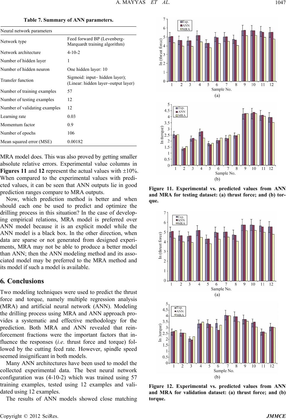
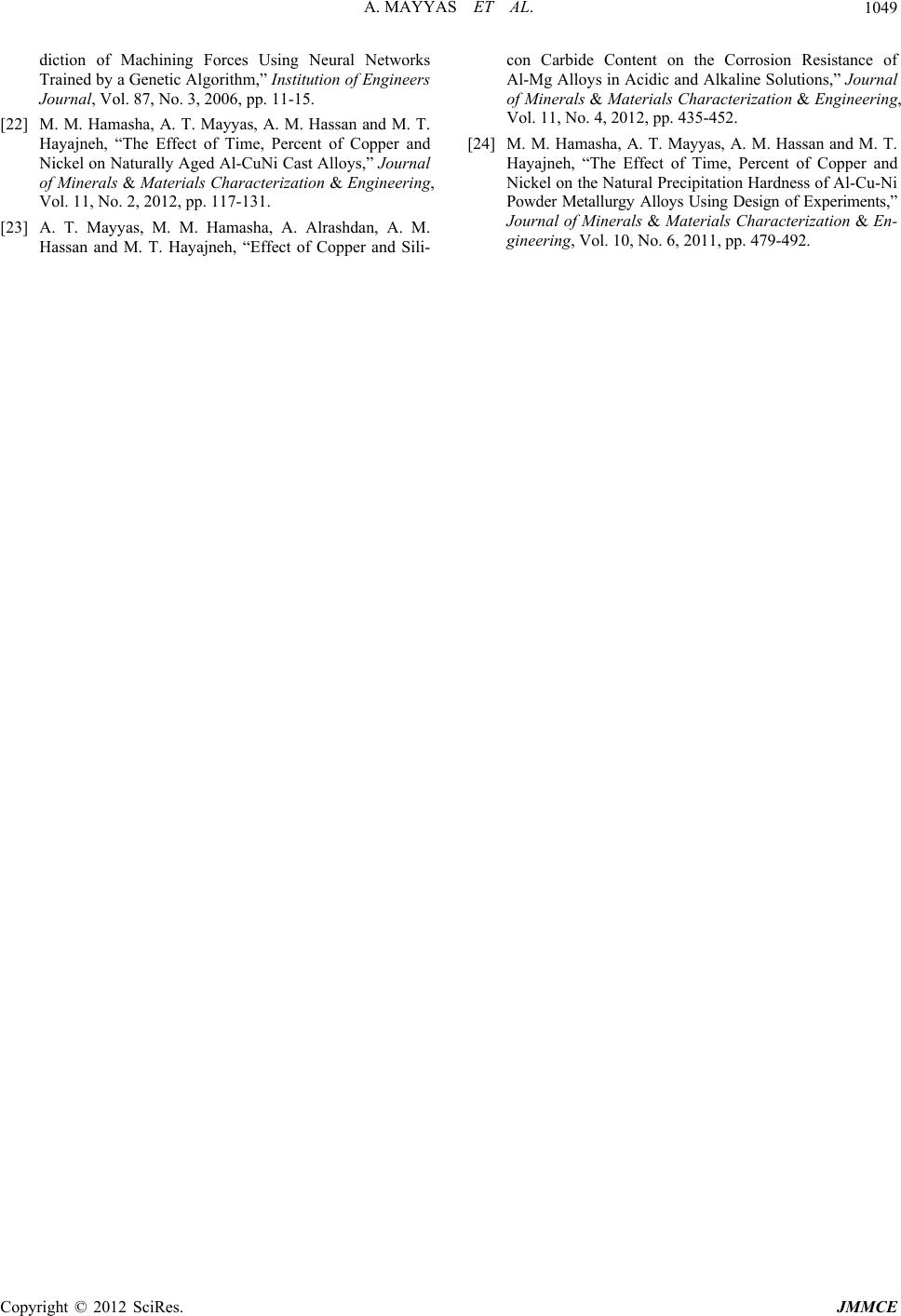
between the model outputs and the measured outputs.
The mean absolute relative errors were 0.82% for torque
and 2.89% for thrust force models, while MRA model
error values were 7.10% and 12.59%, respectively.
Hence, these models can be used efficiently for predic-
tion potentials for non-experimental patterns which, in
turn, save experimental time and cost. It was shown that
ANN performs well in mapping nonlinear relationships
between inputs and outputs. If both MRA and ANN
models are considered they will provide statistically sat-
isfactory prediction results. ANN methodology consumes
less time and gives higher accuracy. Hence, modeling the
drilling process using ANN is more effective compared
with MRA. The two proposed models are good in mod-
eling and predicting the drilling forces, which in turn can
provide a valuable tool for many similar applications of
modeling methods in engineering design and manufac-
turing. The developed modeling methods in this paper
can aid the prediction, optimization, and improvement of
drilling processes and the selection of cutting parameters
in the case of drilling aluminum-based materials.
REFERENCES
[1] J. P. Davim. “Study of Drilling Metal-Matrix Composites
Based on the Taguchi Techniques,” Journal of materials
processing technology, Vol. 132, No. 1-3, 2003, pp. 250-
254. doi:10.1016/S0924-0136(02)00935-4
[2] N. Altinkok and R. Koker. “Use of Artificial Neural Net-
work for Prediction of Physical Properties and Tensile
Strengths in Particle Reinforced Aluminum Matrix Com-
posites,” Journal of Materials Science, Vol. 40, No. 7,
2005, pp. 1767-1770. doi:10.1007/s10853-005-0689-5
[3] N. Altinkok and R. Koker, “Modeling of the Prediction of
Tensile and Density Properties in Particle Reinforced
Metal Matrix Composites by Using Neural Networks,”
Materials & Design, Vol. 27, No. 8, 2006, pp. 625-631.
doi:10.1016/j.matdes.2005.01.005
[4] A. M. Hassan, M. Hayajneh and M. Al-Omari, “The Ef-
fect of the Increase in Graphite Volumetric Percentage on
the Strength and Hardness of Al-4wt%Mg Graphite
Composites,” Journal of Materials Engineering and Per-
formance, Vol. 11, No. 3, 2002, pp. 250-255.
doi:10.1361/105994902770344024
[5] A. M. Hassan, A. Alrashdan, M. T. Hayajneh, A. T. May-
yas, “Prediction of Density, Porosity and Hardness in
Aluminum-Copper-Based Composite Materials Using
Artificial Neural Network,” Journal of materials proc-
essing technology, Vol. 209, No. 2, 2009, pp. 894-899.
doi:10.1016/j.jmatprotec.2008.02.066
[6] S. Kalpakjian and S. R. Schmid, “Manufacturing Engi-
neering and Technology,” 4th Edition, Addison-Wesley,
Boston, 2000.
[7] M. Ramulu, P. N. Rao and H. Kao, “Drilling of
(Al2O3)p/6061 Metal Matrix Composites,” Journal of ma-
terials processing technology, Vol. 124, No. 1-2, 2002,
pp. 244-254. doi:10.1016/S0924-0136(02)00176-0
[8] J. F. Kelly and M. G. Cotterell, “Minimal Lubrication
Machining of Aluminum Alloys,” Journal of Materials
Processing Technology, Vol. 120, No. 1-3, 2002, pp. 327-
334. doi:10.1016/S0924-0136(01)01126-8
[9] M. Tash, F. H. Samuel, F. Mucciardi, H. W Doty and S.
Valtierra, “Effect of Metallurgical Parameters on the Hard-
ness and Microstructural Characterization of As-Cast and
Heat-Treated 356 and 319 Aluminum Alloys,” Materials
Science and Engineering: A, Vol. 443, No. 1-2, 2007, pp.
185-201. doi:10.1016/j.msea.2006.08.054
[10] M. Nouari, G. List, F. Girot and D. Coupard, “Experi-
mental Analysis and Optimisation of Tool Wear in Dry
Machining of Aluminium Alloys,” Wear, Vol. 255, No.
7-12, 2003, pp. 1359-1368.
doi:10.1016/S0043-1648(03)00105-4
[11] G. Tosun and M. Muratoglu, “The Drilling of Al/SiCp
Metal-Matrix Composites. Part II: Workpiece Surface In-
tegrity,” Composites Science and Technology, Vol. 64,
No. 10-11, 2004, pp. 1413-1418.
doi:10.1016/j.compscitech.2003.07.007
[12] G. Tosun and M. Muratoglu, “The Drilling of an Al/SiCP
Metal-Matrix Composites. Part I: Microstructure,” Com-
posites Science and Technology, Vol. 64, No. 2, 2004, pp.
299-308. doi:10.1016/S0266-3538(03)00290-2
[13] J. T. Lin, D. Bharracharyya and V. Kecman, “Multiple
Regression and Neural Networks Analysis in Composite
Machining,” Composite Science and Technology, Vol. 63,
No. 3-4, 2003, pp. 539-548.
doi:10.1016/S0266-3538(02)00232-4
[14] M. T. Hayajneh, A. M. Hassan, A. Alrashdan and A. T.
Mayyas, “Prediction of Tribological Behavior of Alumi-
num-Copper Based Composite Using Artificial Neural
Network,” Journal of Alloys and Compounds 2009, Vol.
470, No. 1-2, 2009, pp. 584-588.
doi:10.1016/j.jallcom.2008.03.035
[15] S. Frouzan and A. Akbarzadeh, “Prediction of Effect of
Thermo-Mechanical Parameters on Mechanical Properties
and Anisotropy of Aluminum Alloy AA3004 Using Arti-
ficial Neural Network,” Materials & Design, Vol. 28, No.
5, 2007, pp. 1678-1684.
doi:10.1016/j.jallcom.2008.03.035
[16] K.Genel, S. C. Kurnaz and M. Durman, “Modeling of
Tribological Properties of Alumina Fiber Reinforced
Zinc-Aluminum Composites Using Artificial Neural Net-
work,” Materials Science and Engineering: A, Vol. 363,
No. 1-2, 2003, pp. 203-210.
doi:10.1016/S0921-5093(03)00623-3
[17] D. Montgomery and G. C. Runger, “Applied Statistics
and Probability for Engineers,” John Wiley and Sons,
New York, 2003.
[18] M. Negnevitsky, “Artificial Intelligence,” 2nd Edition,
Addison-Wesley, Boston, 2005.
[19] J. R. Rogier and M. W. Geatz, “Data Mining: A Tuto-
rial-Based Primer,” Addison-Wesley, Boston, 2003.
[20] Z. Zhang, K. Friedrich and K. Velten, “Prediction on
Tribological Properties of Short Fiber Composites Using
Artificial Neural Networks,” Wear, Vol. 252, No. 7-8,
2002, pp. 668-675. doi:10.1016/S0043-1648(02)00023-6
[21] S. Kumanan, S. K. N. Saheb and C. P. Jesuthanam, “Pre-
Copyright © 2012 SciRes. JMMCE
A. MAYYAS ET AL.
Copyright © 2012 SciRes. JMMCE
1049
diction of Machining Forces Using Neural Networks
Trained by a Genetic Algorithm,” Institution of Engineers
Journal, Vol. 87, No. 3, 2006, pp. 11-15.
[22] M. M. Hamasha, A. T. Mayyas, A. M. Hassan and M. T.
Hayajneh, “The Effect of Time, Percent of Copper and
Nickel on Naturally Aged Al-CuNi Cast Alloys,” Journal
of Minerals & Materials Characterization & Engineering,
Vol. 11, No. 2, 2012, pp. 117-131.
[23] A. T. Mayyas, M. M. Hamasha, A. Alrashdan, A. M.
Hassan and M. T. Hayajneh, “Effect of Copper and Sili-
con Carbide Content on the Corrosion Resistance of
Al-Mg Alloys in Acidic and Alkaline Solutions,” Journal
of Minerals & Materials Characterization & Engineering,
Vol. 11, No. 4, 2012, pp. 435-452.
[24] M. M. Hamasha, A. T. Mayyas, A. M. Hassan and M. T.
Hayajneh, “The Effect of Time, Percent of Copper and
Nickel on the Natural Precipitation Hardness of Al-Cu-Ni
Powder Metallurgy Alloys Using Design of Experiments,”
Journal of Minerals & Materials Characterization & En-
gineering, Vol. 10, No. 6, 2011, pp. 479-492.