Received 24 September 2014; revised 12 October 2014; accepted 24 October 2014

ABSTRACT

Motivated by the lack of a suitable constructive framework for analyzing popular stochastic models of Systems Biology, we devise conditions for existence and uniqueness of solutions to certain jump stochastic differential equations (SDEs). Working from simple examples we find reasonable and explicit assumptions on the driving coefficients for the SDE representation to make sense. By “reasonable” we mean that stronger assumptions generally do not hold for systems of practical interest. In particular, we argue against the traditional use of global Lipschitz conditions and certain common growth restrictions. By “explicit”, finally, we like to highlight the fact that the various constants occurring among our assumptions all can be determined once the model is fixed. We show how basic long time estimates and some limit results for perturbations can be derived in this setting such that these can be contrasted with the corresponding estimates from deterministic dynamics. The main complication is that the natural path-wise representation is generated by a counting measure with an intensity that depends nonlinearly on the state.

Keywords:

Nonlinear Stability, Perturbation, Continuous-Time Markov Chain, Jump Process, Uncertainty, Rate Equation

1. Introduction

The observation that detailed modeling of biochemical processes inside living cells is a close to hopeless task is a strong argument in favor of stochastic models. Such models are often thought to be more accurate than conventional rate-diffusion laws, yet remain more manageable than, say, descriptions formed at the level of individual molecules. Indeed, several studies [1] -[3] have showed that noisy models have the ability to capture relevant phenomena and to explain actual, observed dynamics.

In this work we shall consider some “flow” properties of a stochastic dynamical system in the form of a quite general continuous-time Markov chain. Since the pioneering work of Gillespie [4] [5] , in the Systems Biology context this type of model is traditionally described in terms of a (chemical) master equation (CME). This is the forward Kolmogorov equation of a certain jump stochastic differential equation (jump SDE for brevity), driven by independent point processes with state-dependent intensities. Despite the popularity of the master equation approach, little analysis on a per trajectory-basis of actual models has been attempted.

In the general literature, when discussing existence/uniqueness and various types of perturbation results, different choices of assumptions with different trade-offs have been made. One finds that the treatment often falls into one of two categories taking either a “mathematical” or a “physical” viewpoint. Both of the conditions are highly general but with subsequently less transparent proofs and resulting in more abstract bounds. Or the conditions are formed out of convenience, say, involving global Lipschitz constants, and classical arguments carry through with only minor modifications.

Protter ( [6] Chap. V) offers a nice discussion from the mathematical point of view and in ascending order of generality, including the arguably highly unrestrictive assumption of locally Lipschitz continuous coefficients. Other authors ( [7] , Chap. 6, [8] , Chap. 3-5) also treat the evolution of general jump-diffusion SDEs in conti- nuous state spaces.

A study of the flow properties of jump SDEs is found in [9] , where the setting is scalar and the state is continuous. In [10] jump stochastic partial differential equations are treated, and existence/uniqueness results as well as ergodic results for the case of a multiplicative noise, are found in [11] [12] . Numerical aspects in a similar setting are discussed in [13] .

In a more applied context, stability is often thought of as implied from physical premises and the solution is tactically assumed to be confined inside some bounded region ( [14] , Chap. V). The fundamental issue here is that for open systems in a stochastic setting, there is a non-zero probability of reaching any finite state and global assumptions must be formed with great care. The analysis of open networks under an a priori assumption of boundedness is therefore quite difficult to interpret other than in a qualitative sense. Notable examples in this setting include time discretization strategies [15] [16] , time-parallel simulation techniques [17] , and parameter perturbations [18] .

Evidently, essentially no systems of interest satisfy global Lipschitz assumptions since the fundamental inte- raction almost always takes the form of a quadratic term. Interestingly, for ordinary differential equations, it has been shown [19] that Lipschitz continuous coefficients imply a computationally polynomial-space complete solution; thus providing a kind of explanation for the convenience with this weak feedback assumption. It is also known [20] , that with SDEs, superlinearly growing coefficients may in fact cause the forward Euler method to diverge.

1.1. Agenda

Besides its expository material, the purpose of this paper is to devise simple conditions that imply stability for finite and, in certain cases, infinite times, and that, when applied to systems of practical interest, yield explicit expressions for the associated stability estimates. As a result the framework developed herein applies in a constructive way to any chemical network, of arbitrary size and topology, formed by any combination of the elementary reactions (2.3) to be presented in Section 2. Additionally, it will be clear how to encompass also other types of nonlinear reactions that typically result from adiabatic simplifications.

As an argument in favor of this bottom-up approach one can note that, for evolutionary reasons, biochemical systems tend to operate close to critical points in phase-space where the efficiency is the highest. Clearly, for such dynamical systems, an analysis by analogy might be highly misleading.

We also like to argue that our results are of interest from the modeling point of view. Due to the type of phenomenological arguments often involved, judging the relative effect of the (non-probabilistic) epistemic uncer- tainty is a fundamental issue which has so far not rendered a consistent analysis.

1.2. Outline

The expository material in Section 2 is devoted to formulating the type of processes we are interested in. We state the master equation as well as the corresponding jump SDE and we also look at some simple, yet informative actual examples. Since it is expected that the properties of the stochastic dynamics are somehow similar to those of the deterministic version, we search for a set of minimal assumptions in the latter setting in Section 3. Techniques for finding explicit values of the constants occurring among our assumptions are also devised. The main results of the paper are found in Section 4 where we put our theory together and prove existence and uniqueness, as well as long time estimates and limit results for perturbations. A concluding discussion is found in Section 5.

2. Stochastic Jump Kinetics

In this section we start with the physicist’s traditional viewpoint of pure jump processes and write down the governing master equations. These are evolution equations for the probability densities of continuous-time Markov chains over a discrete state space. Although the application considered here is mesoscopic chemical kinetics, identical or very similar stochastic models are also used in Epidemiology [21] , Genetics [22] and Sociodynamics [23] , to name just a few.

We then proceed with discussing a path-wise representation in terms of a stochastic jump differential equation. The reason the sample path representation is interesting is the possibility to reason about flow properties and thus compare functionals of single trajectories. This is generally not possible with the master equation approach.

For later use we conclude the section by looking at some prototypical models. A simple analysis shows, somewhat surprisingly, that an innocent-looking example produces second moments that grow indefinitely.

2.1. Reaction Networks and the Master Equation

We consider a chemical network consisting of D different chemical species interacting according to R prescribed reaction pathways. At any given time t, the state of the system is an integer vector counting the number of individual molecules of each species. A reaction law is a prescribed change of state with an intensity defined by a reaction propensity,. This is the transition probability per unit of time for moving from the state to:

(2.1)

where is the transition step and is the rth column in the stoichiometric matrix. Informally, for states, we can picture (2.1) as a stochastic version of the time-homogeneous ordinary differential equation

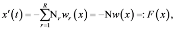(2.2)

where 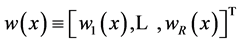is the column vector of reaction propensities.

The physical premises leading to a description in the form of discrete transition laws (2.1) often imply the existence of a system size (e.g. physical volume or total number of individuals). For instance, in a given volume the elementary chemical reactions can be written using the state vector,

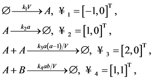(2.3)

with the names of the species in capitals. These propensities are generally scaled such that for some dimensionless function. Intensities of this form are called density dependent and arise naturally in a number of situations ( [24] , Chap. 11). For the rest of this paper, we conveniently take and defer system’s size analysis to another occasion.

The models we consider here all have states in the positive integer lattice and the assumption that no transition can yield a state outside is therefore natural. We make this formal as follows ( [25] , Chap. 8.2.2, Definition 2.4):

Assumption 2.1 (Conservation and stability). For all propensities, for any such that, and we also restrict initial data to. Furthermore, such that is finite for all finite arguments.

To state the chemical master equation (CME), let for brevity be the probability that a certain number of molecules is present at time conditioned upon an initial state. The CME is then given by ( [14] , Chap. V)

(2.4)

The convention of the transpose of the operator to the right of (2.4) is the standard mathematical formulation of Kolmogorov’s forward differential system ( [25] , Chap. 8.3) in terms of which is the infinitesimal generator of the associated Markov process. This is also the adjoint of the master operator in the sense that in the Euclidean inner product over the state space. An explicit representation is

(2.5)

such that the propensities in (2.1) can be retrieved,

(2.6)

Under assumptions to be prescribed in Section 4.1 it holds that the dynamics of the expected value of some time-independent unknown function, conditioned upon the initial state, can be written

(2.7)

We now consider a path-wise representation for the stochastic process.

2.2. The Sample Path Representation

In the present context of analyzing models in stochastic chemical kinetics, the path-wise jump SDE representation seems to have been first put to use in [26] , and it was later further detailed in [16] . It should be noted, however, that an equivalent representation was used much earlier by Kurtz (see the monograph [24] ).

We thus assume the existence of a probability space with the filtration containing - dimensional Poisson processes. The state of the system will be constructed from a stochastic integral with respect to suitably chosen Poisson random measures.

The transition probability (2.1) defines a counting process counting at time the number of reactions of type that has occurred since. It follows that these processes fully determine the state,

(2.8)

The counting processes are obtained from the transition intensities (cf. (2.1))

(2.9)

where by we mean the value of the process prior to any transitions occurring at time, and where the little-o notation is understood uniformly with respect to the state variable. Alternatively, using Kurtz’s random time change representation ( [24] , Chap. 6.2), we can produce the counting process from a standard unit-rate Poisson process,

(2.10)

The marked counting measure ( [27] , Chap. VIII) with defines an increasing sequence of arrival times with corresponding “marks” according to some probability distribution which we will take to be uniform. The intensity of is the Lebesgue measure scaled by the corresponding propensity,. Using this formalism, (2.8) and (2.10) can be written in the jump SDE form

(2.11)

where. Here, the time to the arrival of the next reaction of type is exponentially distributed with intensity. Note that, by virtue of the nature of the propensities, the intensities of the counting processes therefore depend nonlinearly on the state ( [27] , Chap. II.3).

Using that the point processes are independent and therefore have no common jump times ( [25] , Chap. 8.1.3), we can obtain a sometimes more transparent notation in terms of a scalar counting measure. Define for this purpose and for any state the cumulative intensities

(2.12)

such that the total intensity is given by. Let the marks be uniformly distributed on. Then the frequency of each reaction can be controlled through a set of indicator functions defined according to

(2.13)

Put and define also for later use the indicator form

(2.14)

such that

(2.15)

where is defined in (2.2).

The jump SDE (2.11) can now be written in terms of a scalar counting random measure through a state- dependent thinning procedure ( [28] , Chap. 7.5),

(2.16)

Equation (2.16) expresses exponentially distributed reaction times that arrive according to a point process of intensity carrying a mark which is uniformly distributed in. This mark implies the ignition of one of the reaction channels according to the acceptance-rejection rule (2.13).

One frequently decomposes (2.16) into its “drift” and “jump” parts,

(2.17)

The second term in (2.17) is driven by the compensated measure and is a local martingale provided in essence that the path is absolutely integrable (see [27] , Chap. VIII.1, Corollary C4 for details).

2.2.1. Localization: Itô’s and Dynkin’s Formulas

In analytic work it is often necessary to “tame” the process by deriving results under a stopping time in some norm. Results for the stopped process can then be transferred to the original process by letting under suitable conditions.

Although there are many general versions of Itô’s change of variables formula available in the setting of semi- martingales (see for example [8] , Chap. 2.7 and [6] , Chap. II.7), we shall get around with the following simple version ( [7] , Chap. 4.4.2). By the properties of the semi-martingale pure jump process we have for

(2.18)

where the sum is over jump times. Using that we can write this in differential form as

(2.19)

Alternatively, decomposing (2.18) into drift- and jump parts and taking expectation values we get, since the compensated measure is a local martingale,

(18)

This is Dynkin’s formula ( [25] , Chap. 9.2.2) for the stopped process and we note that (2.7) is just a differential version.

2.2.2. Coupled Processes

When considering stability properties we will need to compare different trajectories with respect to the same noise. The details of this coupling are not defined in either (2.11) or (2.16) and must in fact be chosen explicitly. Since this equality is easy to inspect for a unit-rate Poisson process, the viewpoint of local time expressed in (2.10) provides an answer; two processes and may be regarded as coupled if and only if they are evolved using identical Poisson processes, in (2.8) and (2.10). This approach was first used by Kurtz [29] in the context of the random time change representation. Algorithmically it implies the Common Reaction Path (CRP) method for simulating coupled processes [30] (see also [17] ).

A refinement of this construction was devised, also by Kurtz, in ( [31] , see Equations (2.2), (2.3)). In turn, this approach implies the Coupled Finite Difference method [18] (but see also [16] [26] ), and is more amenable to analysis. This is also the construction formalized below under our current framework.

To obtain such a coupled version of (2.16) we will have to make the thinning dependent on both trajectories. This is achieved by firstly replacing the cumulative intensities in (2.12) with the base (or minimal) intensities

(2.21)

and use the new total base intensity as the intensity of the counting measure;. We also modify (2.13) accordingly,

(2.22)

Secondly, we also define the remainder intensity,

(2.23)

In analogy with the previous construction we have the associated total intensity and counting measure;. This time the thinning procedure is non-symmetric in its two first arguments,

(2.24)

with the non-symmetricity due to

(2.25)

As a concrete example of how this comparative thinning might be used, consider the following variant of (2.19),

(2.26)

For this specific example, the terms governed by the base counting measure cancel out altogether.

We mention also that an equivalent construction, but one that leads to different algorithms, can be obtained via a thinning of a single measure [16] [26] . Defining instead

(2.27)

implying the total intensity and associated counting measure; . By construction the indicator functions are now non-symmetric in their first two arguments,

(2.28)

In analogy to (2.26) we get

(2.29)

This time, however, the intensity of the counting measure is generally larger and the equivalence is obtained as a result of the thinning procedure.

2.2.3. The Validity of the Master Equation

With this much formalism developed, we may conveniently quote the following result:

Theorem 2.1 ( [25] , Chap. 8.3.2, Theorem 3.3). Under Assumption 2.1, and if additionally, for it holds that

(2.30)

then (2.7) is valid for.

Since the governing Equation (2.7) for the expected value of is a direct consequence of (2.4), we can similarly conclude the following:

Corollary 2.2 Under the assumptions of Theorem 2.1, and if, moreover, in an arbitrary norm,

(2.31)

then (2.7) is valid for.

In stating these results we have suppressed the conditional dependency on the initial state which we for simplicity consider to be some non-random state.

2.3. Concrete Examples

Consider the bi-molecular birth-death system,

(2.32)

that is, the system is in contact with a large reservoir such that - and -molecules are emitted at a constant rate. Additionally, a decay reaction happens with probability per unit of time whenever two molecules meet. For this example we have the stoichiometric matrix

and the vector propensity function

where.

For a state, define. Itô’s formula (2.19) with yields

(2.33)

which upon a moments consideration is just the same thing as the model

(2.34)

that is, a constant intensity discrete random walk process. An explicit solution is the difference between two independent Poisson distributions,

(2.35)

where is a normally distributed random variable of the indicated mean and variance. Hence fluctuates between arbitrarily large and small values as.

Reversible Versions

From time to time below we shall be concerned with the following closed version of (2.32), consisting of a single reversible reaction,

(2.36a)

This is clearly a finite system since the number is always preserved. An open version of the same system is

(2.36b)

and will prove to be a useful example in the stochastic setting since formally, all states in are reachable. For (2.36a) we have

(2.37)

while (2.36b) is represented by

(2.38)

These examples, while very simple to deal with, will provide good counterexamples in both Sections 3 and 4.

3. Deterministic Stability

In this section we shall be concerned with the deterministic drift part of the dynamics (2.17). We are interested in techniques for judging the stability of the time-homogeneous ODE (2.2), the so-called reaction rate equations implied by the rates (2.1). Stability and continuity with respect to initial data are considered in Sections 3.1 and 3.2. The main motivation for this discussion stems from the observation that assumptions that do not hold in this very basic setting are unlikely to hold in the stochastic case. In Section 3.3, techniques for explicitly obtaining all our postulated constants are discussed. A good point in favor of taking the time to describe these techniques is that we have not found such a discussion elsewhere.

Initially we will consider states, but we will soon find it convenient to restrict the treatment to. In order to remain valid also in the discrete stochastic setting, however, constructed counterexamples will remain relevant also when restricted to.

3.1. Stability

Many stability proofs can be thought of as comparisons with relevant linear cases. This is the motivation for the well-known Grönwall’s inequality which we state in the following two versions.

Lemma 3.1. Suppose that for. Then

(3.1)

The same conclusion holds irrespective of the differentiability of but with and under the weaker integral condition

(3.2)

The most immediate way of comparing the growth of solutions to the ODE (2.2) to those of a linear ODE is to require that the norm of the driving function is bounded in terms of its argument;

(3.3)

since then by the triangle inequality,

(3.4)

where Grönwall’s inequality applies. Unfortunately, (3.3) is a too strict requirement for our applications.

Proposition 3.2 The bi-molecular birth-death system (2.32) does not satisfy (3.3).

Proof. We compute for a state. Hence for a = b = N = 0, 1,··· we have for large enough that, which can clearly never be bounded linearly in.

The problem with the simple condition (3.3) is that it does not take the direction of growth into account; the offending quadratic propensity in (2.32) actually decreases the number of molecules. To deal with this, let be an arbitrary vector defining an “outward” direction. The length of the component of the driving function along this direction is and in order not to have driven too strongly out along this ray we may, in view of Grönwall’s inequality, naturally require that for sufficiently large. Equivalently, for any x,

(3.5)

from which one deduces

(3.6)

where Grönwall’s inequality applies anew. The assumption (3.5) is weaker than (3.3) since the former implies the latter by the Cauchy-Schwarz inequality. Indeed, as in the proof of Proposition 3.2 it is readily checked that for the bi-molecular birth-death system (2.32), we get which this time readily can be bounded linearly in terms of.

Unfortunately, in the case of an infinite state space and strong dependencies between the species the assumption (3.5) is also often unrealistic.

Proposition 3.3 Neither (2.36a) nor (2.36b) admits a bound of the kind (3.5).

Proof. As in the proof of Proposition 3.2 we look at a ray parametrized by a non- negative integer. For (2.36a) we compute, which clearly cannot be bounded linearly in. The same argument applies also to (2.36b).

This negative result can perhaps best be appreciated as a kind of loss of information about the dependencies between the species in the functional form of the condition (3.5). The number of - and -molecules is strongly correlated with the number of -molecules such that, in fact, in (2.36a) is a preserved quantity. By contrast, in (3.5) the growth of is estimated from the sum of the growth of the individual elements of x as if they where independent.

A way around this limitation can be found provided that we leave the general case. We therefore specify the discussion to the positive quadrant and assume from now on that it can be shown a priori that the initial data belongs to this set and that the subsequent trajectory never leaves it (compare Assumption 2.1).

It then follows that, where is the vector of length containing all ones. This vector also defines a suitable “outward” vector for states since solutions to the ODE (2.2) cannot grow without simultaneously growing also in the direction of.

Again, in view of Grönwall’s inequality Lemma 3.1, we tentatively require that for sufficiently large. Equivalently, for any,

(3.7)

implying the bounded dynamics

(3.8)

We remark in passing that the criterion (3.7) is sharp in the sense that if the reversed inequality can be shown to be true, then the growth of solutions can be estimated from below.

Example 3.1 As a point in favor of this approach we compute for the bi-molecular birth-death system (2.32), which evidently falls under the assumption (3.7) with. For the reversible case (2.36a) we similarly get such that (3.7) applies with. Finally, and in the same fashion, the open case (2.36b) is seen to be covered by letting.

The chosen “outward” vector is by no means special. Clearly, any strictly positive vector may be used in its place since and are equivalent norms over. This is a general and useful observation as it may be used to discard parts of a system that are closed without any restrictions on the associated propensities.

Example 3.2 For the reversible system (2.36a), we have already noted that is a conserved quantity such that the choice yields. The open case (2.36b) also benefits from this weighted norm in that we get.

Example 3.3 A slightly more involved model reads as follows:

This example has been constructed such that the quadratic reaction increases and hence (3.7) does not apply. However, taking we get

This example hints at a general technique for obtaining suitable candidates for the weight vector. Simply form the matrix consisting of the columns of that are affected by superlinear propensities. If a vector annihilating these propensities exists, it can be found in the null-space of, readily available by linear algebra techniques. We omit the details.

3.2. Continuity

For well-posedness of the ODE (2.2) we also need continuity with respect to the initial data. We cannot ask for uniform Lipschitz continuity since clearly implies (3.3) which we have already refuted. For the same reason, a uniform one-sided Lipschitz condition cannot be assumed to hold since it implies (3.5). The problem here is the global nature of the estimate and it therefore seems to be reasonable to localize this assumption. For instance, one might ask for

(3.9)

presumably with some growth restrictions on. Although very general, such an analysis is likely to be less informative when it comes to estimating actual constants in later results. We shall therefore consider the following simpler version,

(3.10)

where the form of has been restricted to better suit the present purposes. Trivially, the norms and are equivalent and hence the specific choice made in (3.10) is just a matter of convenience. Since the idea here is to use a priori bounds on and when deriving perturbation bounds, using (or) is natural.

Theorem 3.4 Suppose that the ODE (2.2) satisfies (3.7) and (3.10) and that initial data implies a solution. Then for any there is a unique such solution. Moreover, define, where and are two trajectories associated with initial data, respectively. Then

(3.11)

Proof. Combining (3.7) with Grönwall’s inequality we get the a priori estimate

Hence the (bounded) solution to

is readily found through its integrating factor. The order estimate is a consequence of the fact that

since the trajectory is continuous.

3.3. Bounds for Elementary Reactions

As briefly discussed by the end of Section 3.1, finding bounds on A and in (3.7) as well as a suitable weight-vector amounts to basic inequalities and some fairly straightforward linear algebra manipulations. In this section we therefore consider precise bounds in (3.10) for the elementary propensities (2.3). Since (3.10) is linear in, a reasonable approach is to consider linear and quadratic propensities separate (constant propensities trivially satisfy (3.10) with).

Proposition 3.5 (linear case) Write a set of linear propensities as, , each with the corresponding stoichiometric vector. Then satisfies

with in terms of the Euclidean logarithmic norm

and the matrix containing the vectors as columns. In particular, in the case of a single linear propensity and, if as is usually the case, is all-zero except for a single rate constant in the nth position, then this reduces to.

Proof. The first assertion is immediate since the smallest such constant by definition is the logarithmic norm (see e.g. [32] ). To compute when has the form indicated, we determine the extremal eigenvalue of. By the (signed) scaling invariance of the logarithmic norm we may without loss of generality take. The spectral relation for an eigenpair can be written as

For non-zero the first relation can be solved for. When inserted into the second relation, using that (or otherwise), we get a quadratic equation for with a single extremal root.

Example 3.4 The simple special case in Proposition 3.5 is generally sharp except for when there are linear reactions affecting all species considered in the model. For example, in a one-dimensional state space, the single decay with propensity allows the optimal value. In general -dimensional space, a chain with unit rate constants of the form, or a closed loop in which the last transition is replaced with, both admit bounds as an inspection of the Gershgorin-discs of shows.

Other than for those special examples, for the most important linear cases, Table 1 summarizes the bounds as obtained from the special case in Proposition 3.5 (with all reaction constants normalized to unity).

Proposition 3.6 (quadratic case). Write a general quadratic propensity as with a symmetric matrix. Then satisfies (3.10) with and

. For the special case that there holds.

Proof. Since is symmetric we have. Hence an explicit expression for is obtained as follows:

The indicated upper bound is derived from the fact that [32] . For the useful special case, define first the vector in terms of, and. Using the fact that the logarithmic norm is sub-additive we can reuse the calculation in the proof of Proposition 3.5,

Example 3.5 The most important quadratic cases are summarized in Table 2. For the dimerizations in the lower half of the table there is also a linear part in (3.10).

Example 3.6 The bi-molecular birth-death model (2.32) admits the constants in (3.10). Similarly, the reversible cases (2.36a) and (2.36b) both obeys (3.10) with

. All these results are sharp except for the open case (2.36b) for which one can

obtain a slightly smaller constant by using the general formula stated in Proposition 3.5.

Example 3.7 As a highly prototypical example we consider the following natural extension of the bi- molecular birth-death model (2.32),

where in this example it is informative to consider the dependence on the system’s size. It is straightforward to show the bounds in (3.7) and hence that the system is effectively bounded despite being of open character. This is seen from the fact that, for states, the dynamics is dissipative in the -norm. Furthermore, from Proposition 3.5 and 3.6 we get the sharp bounds in (3.10). It follows that for states such that, the dynamics is contractive in the Euclidean norm. For density dependent propensities we expect that in any norm as grows, and hence the region of contractivity grows in a relative sense. Intuitively one expects that these results offer an insight into the evolution of the process that is relevant also in the stochastic setting.

4. Stochastic Stability

We now consider the properties of the stochastic jump SDE (2.16). For convenience we start by collecting all assumptions in Section 4.1. In the stochastic setting the requirements for existence and uniqueness are slightly stronger than in the deterministic case such that the one-sided bound (3.10) needs to be augmented with an

unsigned version, implying essentially the assumption of at most quadratically growing propensities. We demonstrate that this assumption is reasonable by constructing a model involving cubic propensities and with unbounded second moments. On the positive side we show in Section 4.2 that the assumptions are strong enough to guarantee finite moments of any order during finite time intervals.

We prove existence and uniqueness of solutions to the jump SDE (2.16) in Section 4.3. A sufficient condition for the existence of asymptotic bounds of the pth order moment is given in Section 4.4 where we also derive some stability estimates.

4.1. Working Assumptions

We state formally the set of assumptions on the jump SDE (14) as follows.

Assumption 4.9 For arguments, , , and weighted norm we assume that

(1) (“bounded growth”),

(2) (“absolutely bounded growth”),

(3),

(4).

The parameters are assumed to be positive (with possibly zero) but we allow also negative values of. The vector is normalized such that; hence the bound is sharp.

After the original draft of the current paper was finished, the author became aware of two other papers discussing very similar conditions [33] [34] . In particular, Assumption 4.1 (1), (2) are also found in ( [33] , Condition (1). In fact, these very conditions can be shown to be exactly what is needed to apply the earlier and quite general theory found in ( [35] , Theorem 7.1).

In Assumption 4.9 (2) the case will merit special attention. For well-posedness it turns out that we will need to require a higher regularity of the initial data when (see Theorem 4.7) and the condition for ergodicity becomes more restrictive (see Theorem 4.9). In practice, implies that opposing quadratic reactions of the type

(4.1)

are impossible. Similarly, when reactions of the type

(4.2)

are excluded.

Note that (2) and (4) are redundant in the sense that they are both implied by (3). However, as we saw in Section 3.3, in (4) it is often possible to find sharper constants and by considering this bound in isolation. Also, although (3) is stronger than (4), it is in particular valid for quadratic propensities as can be seen from the representation used in the proof of Proposition 3.6,

(4.3)

The Danger with Cubic Propensities

Assumption 4.1 (2) specifies the discussion to propensities with at most quadratic growth, at least when measured in the direction of the weight vector. To show that this is natural we now demonstrate that additional care should be taken when considering cubic propensities.

Example 4.2 Consider the model

such that the stoichiometric vector is given by, and hence that the drift.

Proposition 4.1 For the model in Example 4.2, if, then the second moment explodes in finite time.

Proof. Assume that both the second and the third moment are bounded for with. From (2.7) we get the governing equation

such that the growth of the second moment remains bounded only provided that the third moment remains finite. It is convenient to look at the cumulative third order moment. From (2.7),

By the arithmetic-geometric mean inequality, , such that by Jensen’s inequality,

We put and get the differential inequality

which can be integrated and rearranged to produce the bound

(4.4)

Hence the third, and consequently also the second moment explode for some finite whenever.

Interestingly, we note that if, then the probability that the cubic decay transition occurs first is, and if this happens the state of the system will be stuck with a single molecule indefinitely.

4.2. Moment Bounds

In this section we consider general moment bounds derived from (2.20) using localization. To get some guidance, let us first assume that the differential form of Dynkin’s formula (2.7) is valid. Since any trajectory by the basic Assumption 2.1 will belong to, we may use that. Hence from (2.7) with we get that

(4.5)

by Assumption 4.1 (1). Clearly, the differential form of Grönwall’s inequality in Lemma 3.1 applies here. A correct version of this argument unfortunately looses the sign of.

Proposition 4.2 If Assumption 4.1 (1) is true, then

where.

Here and below we shall make use of the stopping time and define.

Proof. From (2.20) with we get that

(4.6)

By the integral form of Grönwall’s inequality in Lemma 3.1 we deduce in terms of that

(4.7)

such that the same bound holds for by letting.

We attempt a similar treatment for obtaining bounds in mean square. Assuming tactically that (2.7) is valid, writing we get after some work that

(4.8)

where We expect from Grönwall’s inequality that grows at most exponentially with whenever

(4.9)

However, this tentative condition is often violated in practice since the second term, and since we already know from Proposition 3.3 that this quantity does not admit bounds in terms of even for very simple problems.

More realistic conditions arise when seeking to bound instead.

Proposition 4.3 If for some constants and,

(4.10)

understood elementwise), then.

The proof of Proposition 4.3 follows the same pattern as for Proposition 4.2, but using this time

in (2.20). The condition (4.10) is typically more realistic than (4.9) since we recognize the term, which under the evidently reasonable Assumption 4.1 (1) is. It follows that if grows at most quadratically with, then this assumption is sufficient to yield bounds in mean square. Stated formally,

Proposition 4.4 Under Assumption 4.1 (1) and (2) the condition (4.10) of Proposition 4.3 is true with and.

Proof. This is straightforward: we get by the assumptions and Hölder’s inequality,

where an application of Young’s inequality yields the indicated bounds.

As a strong point in favor of our running assumptions we now demonstrate that the above reasoning can be generalized: these two conditions implies finite time stability in any order moment. We note that in a recent manuscript [34] , related conditions for the same results are proposed.

Theorem 4.5 (Moment estimate). Under Assumption 4.1 (1) and (2), for any integer,

(4.11)

where is a constant depending on the assumptions and on.

The proof of Theorem 4.5 and some later results will simplify using the following bound.

Lemma 4.6 Let with and. Then for integer we have the bounds

(4.12)

(4.13)

Proof. Both results follow from Taylor expansions;

respectively, where. Using the triangle inequality and the elementary inequality the lemma is proved.

Proof of Theorem 4.5. Using (2.20) with we get

(4.14)

Using Lemma 4.6 (4.12) and Assumption 4.1 (1) and (2) we obtain

where. Expanding and using Young’s inequality with exponents and conjugate exponents,

for some constant which thus depends on the assumptions. Applying Grönwall’s inequality and letting we obtain the stated result.

4.3. Existence and Uniqueness

We shall now prove that the jump SDE (2.16) under Assumption 4.1 has a uniquely defined and locally bounded solution. To this end and following ( [8] , Section 3.1.2), we introduce the following spaces of path-wise locally bounded processes:

(4.15)

Theorem 4.7 (Existence). Let be a solution to (2.16) under Assumption 4.1 (1) and (2) with.

Then if,. If then the conclusion remains under the additional

requirement that.

Proof. Below we let denote a positive constant which may be different on each occasion used. As before we use the stopping time and put. We get from Itô’s formula (with G defined in (4.14))

Since the propensities are bounded for bounded arguments (Assumption 2.1), using the stopping time we find that the jump part is absolutely integrable and hence a local martingale. We estimate its quadratic variation under Assumption 4.1 (2),

(4.16)

(4.17)

(4.18)

where. In (4.16) Lemma 4.6 (4.13) was applied and Assumption 4.1 (2) entered in (4.17). Assume

first that. Then for the drift part we have already constructed a suitable bound in Theorem 4.5 such that

Taking supremum and expectation values we get from Burkholder’s inequality ( [6] , Chap. IV.4) that

Writing we conclude that

By Grönwall’s inequality we have thus shown that can be bounded in terms of the initial data and time. The result now follows by letting and using Fatou’s lemma.

Next assume that. Then we have to rely more directly on Theorem 4.5 in (4.18),

where, although there is now a dependency on, the rest of the argument carries through.

For the case that the initial data is non-deterministic we see that the general quadratic case Assumption 4.1 (2) with requires a one order higher moment of the initial data in order for a solution in to exist.

Theorem 4.8 (Uniqueness) Let Assumption 4.1 (1)-(4) hold true. Then any two paths and coupled according to the description in Section 2.2.2 with are equal.

We shall be using the observation that, for, we have that (referred below to as the “integer inequality”).

Proof. Under the same stopping time as before we get from Itô’s formula using the coupling described in Section 2.2.2 that

From the integer inequality we find that there is a constant depending on such that

Using that and Grönwall’s inequality we conclude that the only solution is the zero solution. Letting and using Fatou’s lemma the statement is therefore proved.

In a certain sense the previous result is trivial; from the Poisson representation (2.8) we see that up to the first explosion, a path is uniquely determined from an initial state and a series of Poisson distributed events. However, and as we shall see below, the above proof is prototypical for more involved situations. An example would be when devising hybrid approximations in continuous state space. Indeed, in the above proof, note that if the integer inequality did not hold we would naturally have to rely on the Cauchy-Schwartz inequality instead. With this leads to bounds of the typical kind

(4.20)

for which is an admissible solution. This observation shows that the integer inequality as used in the proof is crucial; without it the integral inequality (4.19) admits growing solutions.

4.4. Stability

Although Theorem 4.5 shows that any moments are bounded in finite time, a relevant question from the modeling point of view is whether the first few moments remain bounded indefinitely. We give a result to this effect which relies on the existence of solutions in which implies that the differential form (2.7) of Dynkin’s formula may be used (cf. Corollary 2.2) such that in turn the differential Grönwall inequality applies. We mention anew that a very similar result has recently appeared in ( [33] , Theorem 2).

Theorem 4.9 (Ergodicity) Under Assumption 4.1 (1), (2), suppose that

(4.21)

Then for integer, remains bounded as.

Proof. The case is slightly more complicated to obtain so we shall concentrate on this. We omit the case since it follows from (4.5) under the present assumptions. The idea of the proof is to asymptotically

bound with a certain positive constant to be decided upon below. By (2.7) we get with,

(4.22)

by Taylor’s formula for some. Using the assumptions we get the bound

(4.23)

For the first term in (4.23) we get from the scaled Young’s inequality with exponent and conjugate exponent that

for some. As for the second term in (4.23) we first estimate for

Next by the arithmetic-geometric mean inequality we get

provided that we choose as the solution to the equation

(4.24)

Taken together we thus have

Since we may pick a small enough such that the bracketed expression remains negative. By Grönwall’s inequality this then proves the result with. To prove the case the same idea of proof applies and results in

for a certain new constant satisfying an equation similar to (4.24).

We next aim at deriving some stability estimates with respect to perturbations in the reaction coefficients. An early account of this was given by Kurtz in [31] , see also [18] for a recent discussion in a bounded setting. Given the linear dependence on the coefficients, in the elementary reactions (2.3) a suitable model seems to be that a perturbation in a propensity spreads linearly in a relative sense,

(4.25)

We make this formal by requiring that

(4.26)

where is a suitable measure of the total perturbation vector and where the perturbed propensity vector function is given by

(4.27)

The existence of an absolute constant in (4.26) follows from Assumption 4.1 (3). We further conveniently assume that the entire statement of Assumption 4.1 carries over to the perturbed system, and for convenience we shall also assume that all constants are the same. By the triangle inequality and Assumption 4.1 (3) we obtain from (4.26) the bound

(4.28)

with some constant and where the simplification in (4.28) assumes an a priori bound (e.g. stopping time) and additionally requires the integer inequality.

The starting point for the analysis will be Itô’s formula under the coupling described in Section 2.2.2. The techniques used below generalize well to pth order moment estimates, but for ease of exposition we let.

Hence under the model for coefficient perturbations (4.26)-(4.27) we have that

(4.29)

Theorem 4.10 (Continuity). Let two trajectories and be given, with the same initial data and coupled according to the discussion in Section 2.2.2. Let the propensities for be perturbed by as indi- cated in (4.26), (4.27). Then

(4.30)

Proof. We use the stopping time and put. From (4.29) we get

(4.31)

where (4.28) was used. Simplifying further for a bounded we get

Using that and Grönwall’s inequality we conclude that

To get rid of the stopping time we write in terms of indicator functions,

(4.32)

Using we get from Markov’s inequality and the previous estimate

(4.33)

Relying on the existence result in Theorem 4.7 we find that for any given we can select (and hence also) such that the right term is. We can next find such that for all, also the left term is. Hence for all, as claimed.

As a by-product of the proof we see that if the process is bounded, then for large enough the probability in (4.32) is zero.

Corollary 4.11 (Perturbation estimate, bounded version) If in Theorem 4.10, the processes and are bounded, then for a constant,

(4.34)

The constant in (4.34) can be bounded explicitly by inspection of (4.28) and (4.31).

For an unbounded system it is apparently much more difficult to obtain explicit estimates. However, by controlling also the martingale part we can strengthen Theorem 4.10 in another direction.

Theorem 4.12 (Continuity/sup) Under the same assumptions as Theorem 4.10 we have that

(4.35)

Proof. The quadratic variation of the martingale part in (4.29) can be bounded as

after using (4.28) and the integer inequality anew. For the drift part we may use the corresponding bound developed in the proof of Theorem 4.10. After taking supremum and expectation values of (4.29) and using Burkholder's inequality we therefore arrive at

by Grönwall’s inequality and using the notation. We now rely on the same strategy as in the proof of Theorem 4.10 to similarly arrive at

and the conclusion follows as before.

5. Conclusions

We have proposed a theoretical framework consisting of a priori assumptions and estimates for problems in stochastic chemical kinetics. The assumptions are strong enough to guarantee well-posedness for a large and physically relevant class of problems. Long time estimates and limit results for perturbations in rate constants have been studied to exemplify the theory. The assumptions are constructive in the sense that explicit techniques for obtaining all postulated constants have either been worked out in detail or at least indicated. We have seen that the case in Assumption 4.1 (2) is particularly promising from the analysis point of view in that the conditions for existence in Theorem 4.7 and the ergodicity in Theorem 4.9 both can be formulated naturally.

In the course of motivating our setup we have seen that most problems do not admit global Lipschitz constants and that one-sided versions do not provide a better alternative. Another conclusion worth highlighting is that it pays off to consider jump SDEs in a fully discrete setting in that there are potential complications in proving uniqueness in continuous state space. A practical implication is that care should be exercised when forming continuous approximations to these types of jump SDEs.

For future work we intend to re-visit certain classical results from the perspective of the framework developed herein; for example, thermodynamic limit results, time discretization strategies, and quasi-steady state approximations―all of which have a practical impact in a range of applications.

Acknowledgements

The author likes to express his sincere gratitude to Takis Konstantopoulos for several fruitful and clarifying discussions. Early inputs on this work were also gratefully obtained from Henrik Hult, Ingemar Kaj, and Per Lötstedt.

This work was supported by the Swedish Research Council within the UPMARC Linnaeus center of Excellence.

References

- Lestas, I., Vinnicombe, G. and Paulsson, J. (2010) Fundamental Limits on the Suppression of Molecular Fluctuations. Nature, 467, 174-178. http://dx.doi.org/10.1038/nature09333
- Raj, A. and van Oudenaarden, A. (2008) Nature, Nurture, or Chance: Stochastic Gene Expression and Its Consequences. Cell, 135, 216-226. http://dx.doi.org/10.1016/j.cell.2008.09.050
- Samoilov, M.S. and Arkin, A.P. (2006) Deviant Effects in Molecular Reaction Pathways. Nature Biotechnology, 24, 1235-1240. http://dx.doi.org/10.1038/nbt1253
- Gillespie, D.T. (1976) A General Method for Numerically Simulating the Stochastic Time Evolution of Coupled Chemical Reactions. Journal of Computational Physics, 22, 403-434. http://dx.doi.org/10.1016/0021-9991(76)90041-3
- Gillespie, D.T. (1992) A Rigorous Derivation of the Chemical Master Equation. Physica A, 188, 404-425. http://dx.doi.org/10.1016/0378-4371(92)90283-V
- Protter, P.E. (2005) Stochastic Integration and Differential Equations. Number 21 in Stochastic Modelling and Applied Probability. 2nd Edition, Version 2.1, Springer, Berlin.
- Applebaum, D. (2004) Lévy Processes and Stochastic Calculus, Volume 93 of Cambridge Studies in Advanced Mathematics. Cambridge University Press, Cambridge.
- Situ, R. (2005) Theory of Stochastic Differential Equations with Jumps and Applications. Mathematical and Analytical Techniques with Applications to Engineering. Springer, New York.
- Øksendal, B. and Zhang, T. (2007) The Itô-Ventzell Formula and Forward Stochastic Differential Equations Driven by Poisson Random Measures. Osaka Journal of Mathematics, 44, 207-230.
- Hausenblas, E. (2007) SPDEs Driven by Poisson Random Measure with Non Lipschitz Coefficients: Existence Results. Probability Theory and Related Fields, 137, 161-200.
- Marinelli, C., Prévôt, C. and Röckner, M. (2010) Regular Dependence on Initial Data for Stochastic Evolution Equations with Multiplicative Poisson Noise. Journal of Functional Analysis, 258, 616-649. http://dx.doi.org/10.1016/j.jfa.2009.04.015
- Marinelli, C. and Röckner, M. (2010) Well-Posedness and Asymptotic Behavior for Stochastic Reaction-Diffusion Equations with Multiplicative Poisson Noise. Electronic Journal of Probability, 15, 1529-1555. http://dx.doi.org/10.1214/EJP.v15-818
- Filipović, D., Tappe, S. and Teichmann, J. (2010) Jump-Diffusions in Hilbert Spaces: Existence, Stability and Numerics. Stochastics, 82, 475-520. http://dx.doi.org/10.1080/17442501003624407
- van Kampen, N.G. (2004) Stochastic Processes in Physics and Chemistry. 2nd Edition, Elsevier, Amsterdam.
- Higham, D.J. and Kloeden, P.E. (2005) Numerical Methods for Nonlinear Stochastic Differential Equations with Jumps. Numerische Mathematik, 101, 101-119. http://dx.doi.org/10.1007/s00211-005-0611-8
- Li, T.J. (2007) Analysis of Explicit Tau-Leaping Schemes for Simulating Chemically Reacting Systems. Multiscale Modeling & Simulation, 6, 417-436. http://dx.doi.org/10.1137/06066792X
- Engblom, S. (2009) Parallel in Time Simulation of Multiscale Stochastic Chemical Kinetics. Multiscale Modeling & Simulation, 8, 46-68. http://dx.doi.org/10.1137/080733723
- Anderson, D.F. (2012) An Efficient Finite Difference Method for Parameter Sensitivities of Continuous Time Markov Chains. SIAM Journal on Numerical Analysis, 50, 2237-2258. http://dx.doi.org/10.1137/110849079
- Kawamura, A. (2009) Lipschitz Continuous Ordinary Differential Equations Are Polynomial-Space Complete. 24th Annual IEEE Conference on Computational Complexity, Paris, 15-18 July 2009, 149-160.
- Hutzenthaler, M., Jentzen, A. and Kloeden, P.E. (2011) Strong and Weak Divergence in Finite Time of Euler’s Method for Stochastic Differential Equations with Non-Globally Lipschitz Continuous Coefficients. Proceedings of the Royal Society A, 467, 1563-1576.
- Chen, W.Y. and Bokka, S. (2005) Stochastic Modeling of Nonlinear Epidemiology. Journal of Theoretical Biology, 234, 455-470. http://dx.doi.org/10.1016/j.jtbi.2004.11.033
- Ewens, W.J. (2004) Mathematical Population Genetics I. Theoretical Introduction, Volume 27 of Interdisciplinary Applied Mathematics. 2nd Edition, Springer, New York.
- Escudero, C., Buceta, J., de la Rubia, F.J. and Lindenberg, K. (2004) Extinction in Population Dynamics. Physical Review E, 69, 021908.
- Ethier, S.N. and Kurtz, T.G. (1986) Markov Processes: Characterization and Convergence. Wiley Series in Probability and Mathematical Statistics. John Wiley & Sons, New York. http://dx.doi.org/10.1002/9780470316658
- Brémaud, P. (1999) Markov Chains: Gibbs Fields, Monte Carlo Simulation, and Queues. Number 31 in Texts in Applied Mathematics. Springer, New York. http://dx.doi.org/10.1007/978-1-4757-3124-8
- Plyasunov, S. (2005) On Hybrid Simulation Schemes for Stochastic Reaction Dynamics. http://arxiv.org/abs/math/0504477
- Brémaud, P. (1981) Point Processes and Queues: Martingale Dynamics. Springer Series in Statistics. Springer, New York.
- Daley, D.J. and Vere-Jones, D. (2003) An Introduction to the Theory of Point Processes, Volume I: Elementary Theory and Methods. 2nd Edition, Springer, New York.
- Kurtz, T.G. (1978) Strong Approximation Theorems for Density Dependent Markov Chains. Stochastic Processes and Their Applications, 6, 223-240. http://dx.doi.org/10.1016/0304-4149(78)90020-0
- Rathinam, M., Sheppard, P.W. and Khammash, M. (2010) Efficient Computation of Parameter Sensitivities of Discrete Stochastic Chemical Reaction Networks. Journal of Chemical Physics, 132, 034103. http://dx.doi.org/10.1063/1.3280166
- Kurtz, T.G. (1982) Representation and Approximation of Counting Processes. In: Fleming, W.H. and Gorostiza, L.G., Eds., Advances in Filtering and Optimal Stochastic Control, Vol. 42, Lecture Notes in Control and Information Sciences, Springer, Berlin, 177-191.
- Ström, T. (1975) On Logarithmic Norms. SIAM Journal on Numerical Analysis, 12, 741-753. http://dx.doi.org/10.1137/0712055
- Briat, C., Gupta, A. and Khammash, M. (2014) A Scalable Computational Framework for Establishing Long-Term Behavior of Stochastic Reaction Networks. PLoS Computational Biology, 10, e1003669.
- Rathinam, M. (2014) Moment Growth Bounds on Continuous Time Markov Processes on Non-Negative Integer Lattices. To appear in Quart. Appl. Math. http://arxiv.org/abs/1304.5169
- Meyn, S.P. and Tweedie, R.L. (1993) Stability of Markovian Processes III: Foster-Lyapunov Criteria for Continuous- Time Processes. Advances in Applied Probability, 25, 518-548. http://dx.doi.org/10.2307/1427522