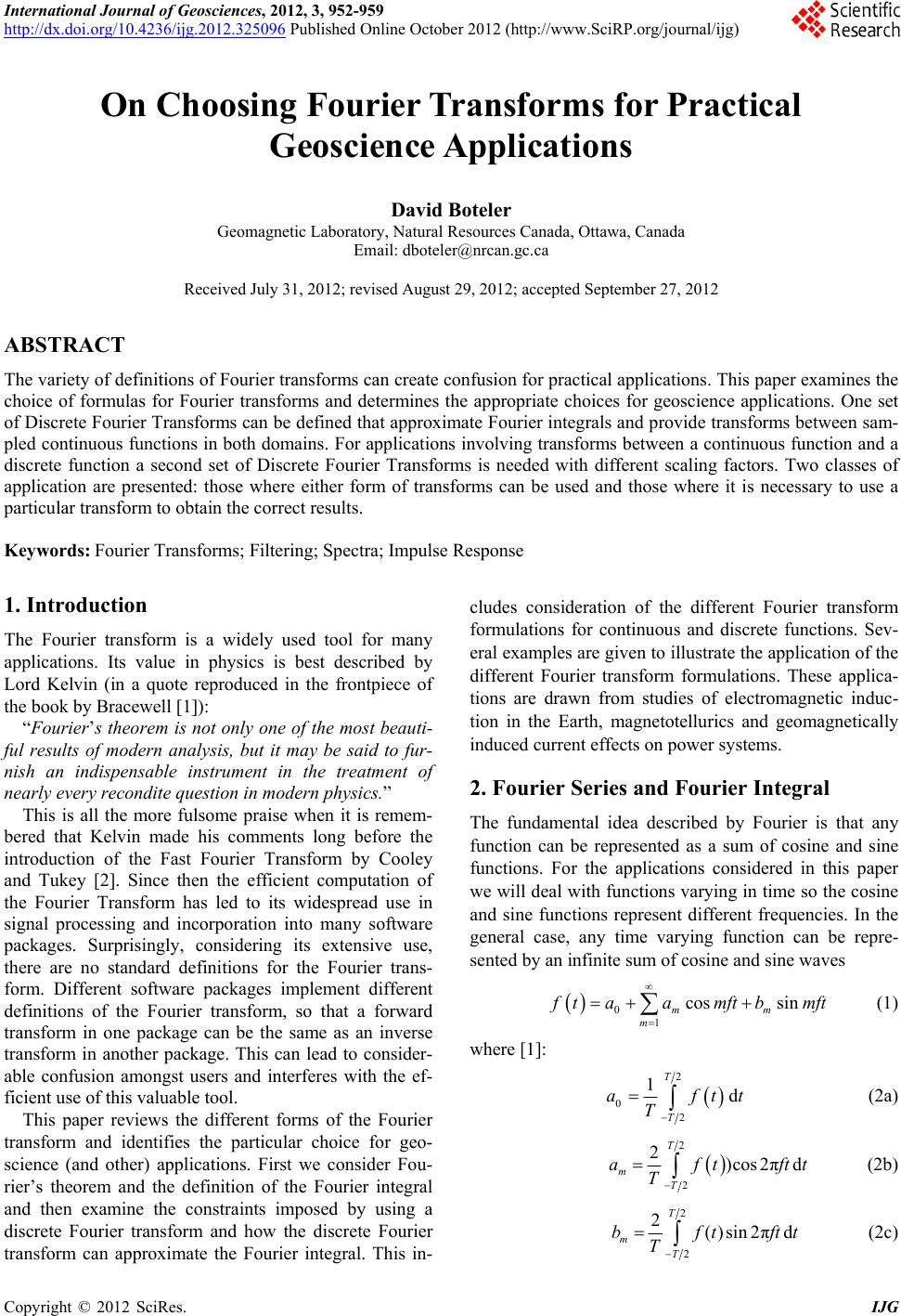International Journal of Geosciences, 2012, 3, 952-959
http://dx.doi.org/10.4236/ijg.2012.325096 Published Online October 2012 (http://www.SciRP.org/journal/ijg)
On Choosing Fourier Transforms for Practical
Geoscience Applications
David Boteler
Geomagnetic Laboratory, Natural Resources Canada, Ottawa, Canada
Received July 31, 2012; revised August 29, 2012; accepted September 27, 2012
ABSTRACT
The variety of definitions of Fourier transforms can create confusion for practical applications. This paper examines the
choice of formulas for Fourier transforms and determines the appropriate choices for geoscience applications. One set
of Discrete Fourier Transforms can be defined that approximate Fourier integrals and provide transforms between sam-
pled continuous functions in both domains. For applications involving transforms between a continuous function and a
discrete function a second set of Discrete Fourier Transforms is needed with different scaling factors. Two classes of
application are presented: those where either form of transforms can be used and those where it is necessary to use a
particular transform to obtain the correct results.
Keywords: Fourier Transforms; Filtering; Spectra; Impulse Response
1. Introduction
The Fourier transform is a widely used tool for many
applications. Its value in physics is best described by
Lord Kelvin (in a quote reproduced in the frontpiece of
the book by Bracewell [1]):
“Fourier’s theorem is not only one of the most beauti-
ful results of modern analysis, but it may be said to fur-
nish an indispensable instrument in the treatment of
nearly every recondite question in modern physics.”
This is all the more fulsome praise when it is remem-
bered that Kelvin made his comments long before the
introduction of the Fast Fourier Transform by Cooley
and Tukey [2]. Since then the efficient computation of
the Fourier Transform has led to its widespread use in
signal processing and incorporation into many software
packages. Surprisingly, considering its extensive use,
there are no standard definitions for the Fourier trans-
form. Different software packages implement different
definitions of the Fourier transform, so that a forward
transform in one package can be the same as an inverse
transform in another package. This can lead to consider-
able confusion amongst users and interferes with the ef-
ficient use of this valuable tool.
This paper reviews the different forms of the Fourier
transform and identifies the particular choice for geo-
science (and other) applications. First we consider Fou-
rier’s theorem and the definition of the Fourier integral
and then examine the constraints imposed by using a
discrete Fourier transform and how the discrete Fourier
transform can approximate the Fourier integral. This in-
cludes consideration of the different Fourier transform
formulations for continuous and discrete functions. Sev-
eral examples are given to illustrate the application of the
different Fourier transform formulations. These applica-
tions are drawn from studies of electromagnetic induc-
tion in the Earth, magnetotellurics and geomagnetically
induced current effects on power systems.
2. Fourier Series and Fourier Integral
The fundamental idea described by Fourier is that any
function can be represented as a sum of cosine and sine
functions. For the applications considered in this paper
we will deal with functions varying in time so the cosine
and sine functions represent different frequencies. In the
general case, any time varying function can be repre-
sented by an infinite sum of cosine and sine waves

0
1
cos sin
mm
m
taamft bmft


 

f
(1)
where [1]:

2
0
2
1d
T
T
aftt
T
 (2a)

2
2
2)cos2πd
T
m
T
aftftt
T
 (2b)
2
2
2()sin2πd
T
m
T
bftftt
T
 (2c)
C
opyright © 2012 SciRes. IJG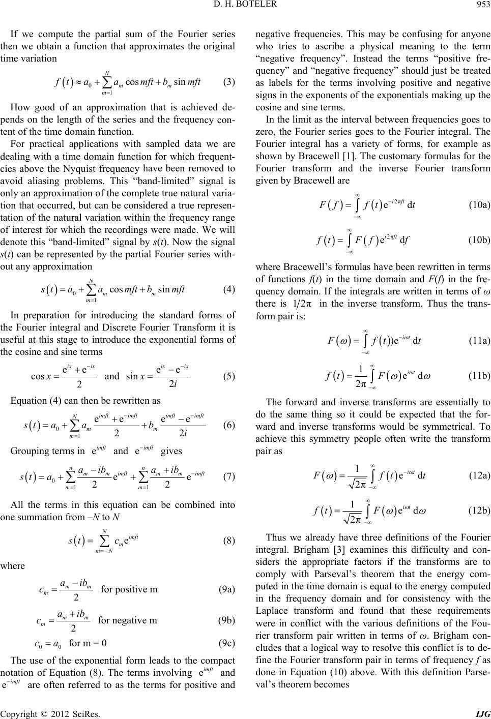

D. H. BOTELER 953
If we compute the partial sum of the Fourier series
then we obtain a function that approximates
time variation
the original

0
1
cos sin
N
mm
m
f
taamft bmft

 
 (3)
How good of an approximation that is achieved de-
pends on the length of the series and the freque
tent of the time domain function.
have been removed to
av
ncy con-
For practical applications with sampled data we are
dealing with a time domain function for which frequent-
cies above the Nyquist frequency
oid aliasing problems. This “band-limited” signal is
only an approximation of the complete true natural varia-
tion that occurred, but can be considered a true represen-
tation of the natural variation within the frequency range
of interest for which the recordings were made. We will
denote this “band-limited” signal by s(t). Now the signal
s(t) can be represented by the partial Fourier series with-
out any approximation

0
1
cos sin
N
mm
m
s
taamftb mft

 
 (4)
In preparation for introducing the standard forms of
the Fourier integral and Discrete Fourier Tra
useful at this stage to introduce the exponential forms of
th
nsform it is
e cosine and sine terms
ee
cos 2
ix ix
x


 and ee
sin 2
ix ix
xi


 (5)
Equation (4) can then be rewritten as

0
12 m
imft
ee ee
2
imft imft
N
mm
st aabi

 
 (6)
Grou erm and e gives
imft imft

ping ts in eimft

0
1m1
ee
22
nn
imft imft mm mm
m
aib aib
st a


 

(7)
All the terms in this equation can be combined into
one summation from –N to N
N
where

eimft
m
mN
st c

 (8)
2
mm
m
aib
 for positive m (9a) c
2
mm
m
aib
c  f
00
ca for m = 0 (9c)
The use of the exp
notation of Equimft
eimft are ofte
ne
the
“neg
riety of forms, for example as
sh
or negative m (9b)
onential form leads to the compact
ation (8). The terms involving e and
n referred to as the terms for positive and
gative frequencies. This may be confusing for anyone
who tries to ascribe a physical meaning to term
ative frequency”. Instead the terms “positive fre-
quency” and “negative frequency” should just be treated
as labels for the terms involving positive and negative
signs in the exponents of the exponentials making up the
cosine and sine terms.
In the limit as the interval between frequencies goes to
zero, the Fourier series goes to the Fourier integral. The
Fourier integral has a va
own by Bracewell [1]. The customary formulas for the
Fourier transform and the inverse Fourier transform
given by Bracewell are
 
2π
ed
ift
F
fft t

 (10a)

 
2π
ed
ift
f
tFf f



where Bracewell’s formulas have been rewritten in terms
of functions f(t) in the time domain
quency domain. If the integrals are written in terms of ω
(10b)
and F(f) in the fre-
there is 12π in the inverse transform. Thus the trans-
form pair is:
 
)e d
it
F
ft t



 (11a)

 
1ed
2π
it
ftF

 (11b)




The forward and inverse transforms are essentially to
do the same thing so it could be expecte
ward and inverse transforms would be symmetrical. To
ac
d that the for-
hieve this symmetry people often write the transform
pair as
 
1ed
it
2π
F
ft t



 (12a)

 
1ed
2π
it
ft F






Thus we already have three definitions
integral. Brigham [3] examines this diff
siders the appropriate factors if the transforms are to
co
(12b)
of the Fourier
iculty and con-
mply with Parseval’s theorem that the energy com-
puted in the time domain is equal to the energy computed
in the frequency domain and for consistency with the
Laplace transform and found that these requirements
were in conflict with the various definitions of the Fou-
rier transform pair written in terms of ω. Brigham con-
cludes that a logical way to resolve this conflict is to de-
fine the Fourier transform pair in terms of frequency f as
done in Equation (10) above. With this definition Parse-
val’s theorem becomes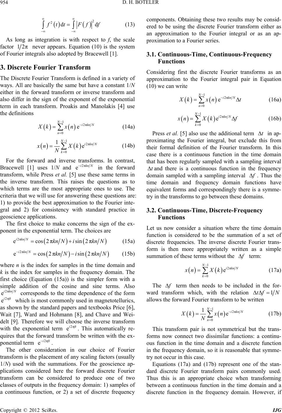

D. H. BOTELER 954
 
2
2dd
f
ttFf f

 

 (13)
As long as integration is with respect to f, the scale
factor 12π never appears. Equation (10)
of Fourier integrals also adopted by Bracewell [1].
ety of
ve a constant 1/N
se transform and
is the system
3. Discrete Fourier Transform
The Discrete Fourier Transform is defined in a vari
ways. All are basically the same but ha
either in the forward transform or inver
also differ in the sign of the exponent of the exponential
term in each transform. Proakis and Manolakis [4] use
the definitions
 
12π
0
e
NiknN
n
Xk xn


 (14a)
 
1
0
1N
k
xn N


2π eik
nN
X k
For the forward and inverse transforms. In contrast,
Bracewell [1] uses and
(14b)
1/N2π eiknN
transform, whil [5] use these same terms in
th
priate
in the forward
e Press et al.
e inverse transform. This raises the questions as to
which terms are the most approones to use. The
criteria that we will use for answering these questions are:
1) to provide the best approximation to the Fourier inte-
gral and 2) for consistency with standard practice in
geoscience applications.
The first choice to make concerns the sign of the ex-
ponent in the exponential term. The choices are

sin2 πNiknN (15a)
2π
ecos2π
iknN kn

2π
ecos2πsin2 π
iknN kn NiknN  (15b)
where n is the index for samples in the time
k is the index for samples in the frequency do
first choice (Equation (15a)) is the simpler fo
domain and
main. The
rm with a
simple addition of the cosine and sine terms. Also
2π
eiknN corresponds to the time dependence of the form
2π
eift which is most commonly used in magnetotellurics,
as shown by the standard papers and textbooks Price [6],
Wai7], Ward and Hohmann [8], and Chave and Wei-
]. Therefore we will choose the inverse transform
with the exponential term 2π
eift . This automatically re-
quires that the forward transform be written with the ex-
ponential term 2π
eift.
The other considerationour choice of Fourier
transform is the placement of any scaling factors (usually
1/N) used with thummations. For the geoscience ap-
pl
t [
delt [9
in
e s
urier transforms as an
on
ications considered here the forward discrete Fourier
transform can be considered to produce one of two
classes of outputs in the frequency domain: 1) samples of
a continuous function, or 2) a set of discrete frequency
components. Obtaining these two results may be consid-
ered to be using the discrete Fourier transform either as
an approximation to the Fourier integral or as an ap-
proximation to a Fourier series.
3.1. Continuous-Time, Continuous-Frequency
Functions
Considering first the discrete Fo
approximation to the Fourier integral pair in Equati
(10) we can write
 
1N2π
0
eik
nN
n
X
kxn t





 (16a)
 
12π
0
e
NiknN
k
x
nXkf




 (16b)
Press et al. [5] also use the additional term t

in ap-
proximating the Fourier integral, but exclude this from
their formal definition of the Fourier
case there is a continuous function in the time domain
thg
transform. In this
at has been regularly sampled with a samplininterval
t

and there is a continuous function in the frequency
domain sampled with a sampling interval
f
. Thus the
time domain and frequency domain functions have
equivalent forms and correspondingly there is a symme-
in the transforms to go between these domains.
3.2. Continuous-Time, Discrete-Frequency
Functions
Let us now consider a situation where the time do
try
main
set of
trans-
formre appropriately written as a simple
function is considered to be the summation of a
discrete frequencies. The inverse discrete Fourier
is then mo
summation of these terms without the
f
 term:
 
12π
0
e
NiknN
k
xnXk


 (17a)
The
f

term then needs to be included in the for-
ward transform which, with the relation 1tf N 
allows the forward Fourier transform to be written
 
12π
0
1e
NiknN
n
Xk xn
N


 (17b)
This transform pair is not symmetrical but the trans-
forms now connect two dissimilar functions: a continu-
ous function in the time domain and a d
in the frequency domain, so it is reasonable that symme-
try
ction in the time domain and a
di
iscrete function
not occur in this case.
Equations (17a) and (17b) represent one of the stan-
dard discrete Fourier transform pairs commonly used.
Thus this is an appropriate choice when transforming
between a continuous fun
screte function in the frequency domain. However, if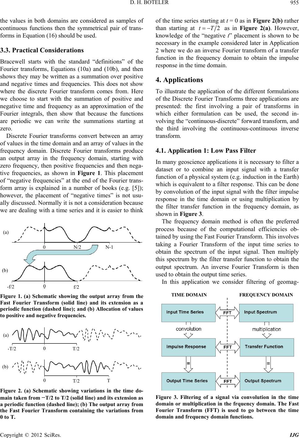

D. H. BOTELER 955
the values in both domains are considered as samples of
continuous functions then the symmetrical pair of trans-
forms in Equation (16) should be used.
3.3. Practical Considerations
Bracewell starts with the standard “definitions” of the
Fourier transforms, Equations (10a) and (10b), and then
mmation over positive
s. This does not show
tput array in the frequency domain, starting with
ze
shows they may be written as a su
and negative times and frequencie
where the discrete Fourier transform comes from. Here
we choose to start with the summation of positive and
negative time and frequency as an approximation of the
Fourier integrals, then show that because the functions
are periodic we can write the summations starting at
zero.
Discrete Fourier transforms convert between an array
of values in the time domain and an array of values in the
frequency domain. Discrete Fourier transforms produce
an ou
ro frequency, then positive frequencies and then nega-
tive frequencies, as shown in Figure 1. This placement
of “negative frequencies” at the end of the Fourier trans-
form array is explained in a number of books (e.g. [5]);
however, the placement of “negative times” is not usu-
ally discussed. Normally it is not a consideration because
we are dealing with a time series and it is easier to think
0 N/2 N-1
f/2
-f/2 0
(a)
(b)
Figure 1. (a) Schematic showing the output array from the
Fast Fourier Transform (solid line) and its extension as a
periodic function (dashed line); and (b) Allocation of values
to positive and negative frequencies.
0 T/2
T
-T/2
0
(a)
(b)
T/2
Figure 2. (a) Schematic showing variations in the time do-
main taken from −T/2 to T/2 (solid line) and its extension as
a periodic function (dashed line); (b) The output array from
the Fast Fourier Transform containing the variations from
0 to T.
of the time series starting at t = 0 as in Figure 2(b) rather
than starting at 2tT

 as in Figure 2(a). However,
knowledge of the “negative t” placement is shown to be
necessary in the example considered later in Application
2 where we do an inverse Fourier transform of a transfer
function in the fr domain to obtain the impulse
response in the time domain.
4. Applications
To illustrate the application of the different formulations
of the Discrete Fourier Transf
equency
orms three applications are
involving a pair of transforms in
lation can be used, the second in-
to combine an input signal with a transfer
function of a physical system (e.g. induction in the Earth)
his can be done
presented: the first
which either formu
volving the “continuous-discrete” forward transform, and
the third involving the continuous-continuous inverse
transform.
4.1. Application 1: Low Pass Filter
In many geoscience applications it is necessary to filter a
dataset or
which is equivalent to a filter response. T
by convolution of the input signal with the filter impulse
response in the time domain or using multiplication by
the filter transfer function in the frequency domain, as
shown in Figure 3.
The frequency domain method is often the preferred
process because of the computational efficiencies ob-
tained by using the Fast Fourier Transform. This involves
taking a Fourier Transform of the input time series to
obtain the spectrum of the input signal. Then multiply
this spectrum by the filter transfer function to obtain the
output spectrum. An inverse Fourier Transform is then
used to obtain the output time series.
In this application we consider filtering of geomag-
TIME DOMAIN FREQUENCY DOMAIN
Figure 3. Filtering of a signal via convolution in the time
domain or multiplication in the frquency domain. The Fast
Fourier Transform (FFT) is used to go between the time
domain and frequency domain functions.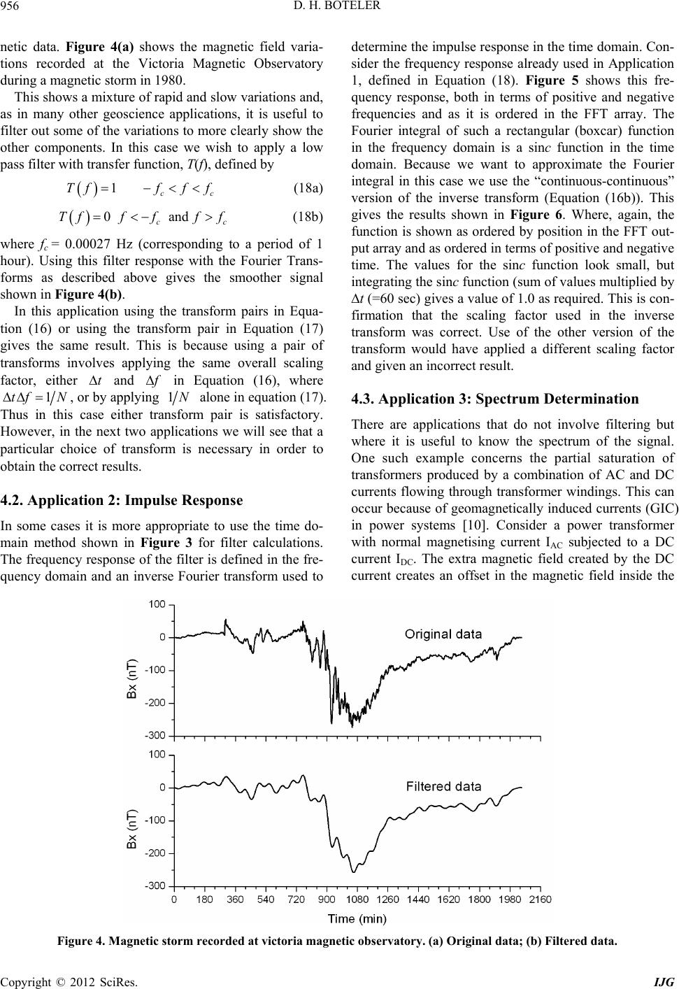

D. H. BOTELER 956
netic data. Figure 4(a) shows the magnetic field varia-
tions recorded at the Victoria Magnetic Observatory
during a magnetic storm in 1980.
This shows a mixture of rapid and slow variations and,
as in many other geoscience applications, it is useful to
filter out some of the variations to more clearly show the
other components. In this case we wish to apply a low
pass filter with transfer function, T(f), defined by
cc
ff f (18a)
0and
cc
fff  (18b)
where fc = 0.00027 Hz (corresponding to a period of
determine the impulse response in the time domain. Con-
sider the frequency response already used in Application
1, defined in Equation (18). Figure 5 shows this fre-
quency response, both in terms of positive and negative
frequencies and as it is ordered in the FFT array. The
Fourier integral of such a rectangular (boxcar) function
in the frequency domain is a sinc function in the time
domain. Because we want to approximate the Fourier
integral in this case we use the “continuous-continuous”
version of the inverse transform (Equation (16b)). This
gives the results shown in Figure 6. Where, again, the
function is shown as ordered by position in the FFT out-
put array and as ordered in terms of positive and negative
time. The values for the sinc function look small, but
integrating the sinc function (sum of values multiplied by
∆t (=60 sec) gives a value of 1.0 as required. This is con-
firmation that the scaling factor used in the inverse
transform was correct. Use of the other version of the
transform would have applied a different scaling factor
and given an incorrect result.

1Tf

Tf f
1
hour). Using this filter response with the Fourier Trans-
forms as described above gives the smoother signal
shown in Figure 4(b).
In this application using the transform pairs in Equa-
tion (16) or using the transform pair in Equation (17)
gives the same result. This is because using a pair of
transforms involves applying the same overall scaling
factor, either t and
f
 in Equation (16), where
1tf N , or by applying 1N alone in equation (17).
Thus in this case either transform pair is satisfactory.
However, in the next two applications we will see that a
particular choice of transform is necessary in or
4.3. Application 3: Spectrum Determination
There are applications that do not involve filtering but
where it is useful to know the spectrum of the signal.
One such example concerns the partial saturation of
transformers produced by a combination of AC and DC
currents flowing through transformer windings. This can
occur because of geomagnetically induced currents (GIC)
in power systems [10]. Consider a power transformer
with normal magnetising current IAC subjected to a DC
current IDC. The extra magnetic field created by the DC
current creates an offset in the magnetic field inside the
der to
obtain the correct results.
4.2. Application 2: Impulse Response
In some cases it is more appropriate to use the time do-
main method shown in Figure 3 for filter calculations.
The frequency response of the filter is defined in the fre-
quency domain and an inverse Fourier transform used to
Figure 4. Magnetic storm recorded at victoria magnetic observatory. (a) Original data; (b) Filtered data.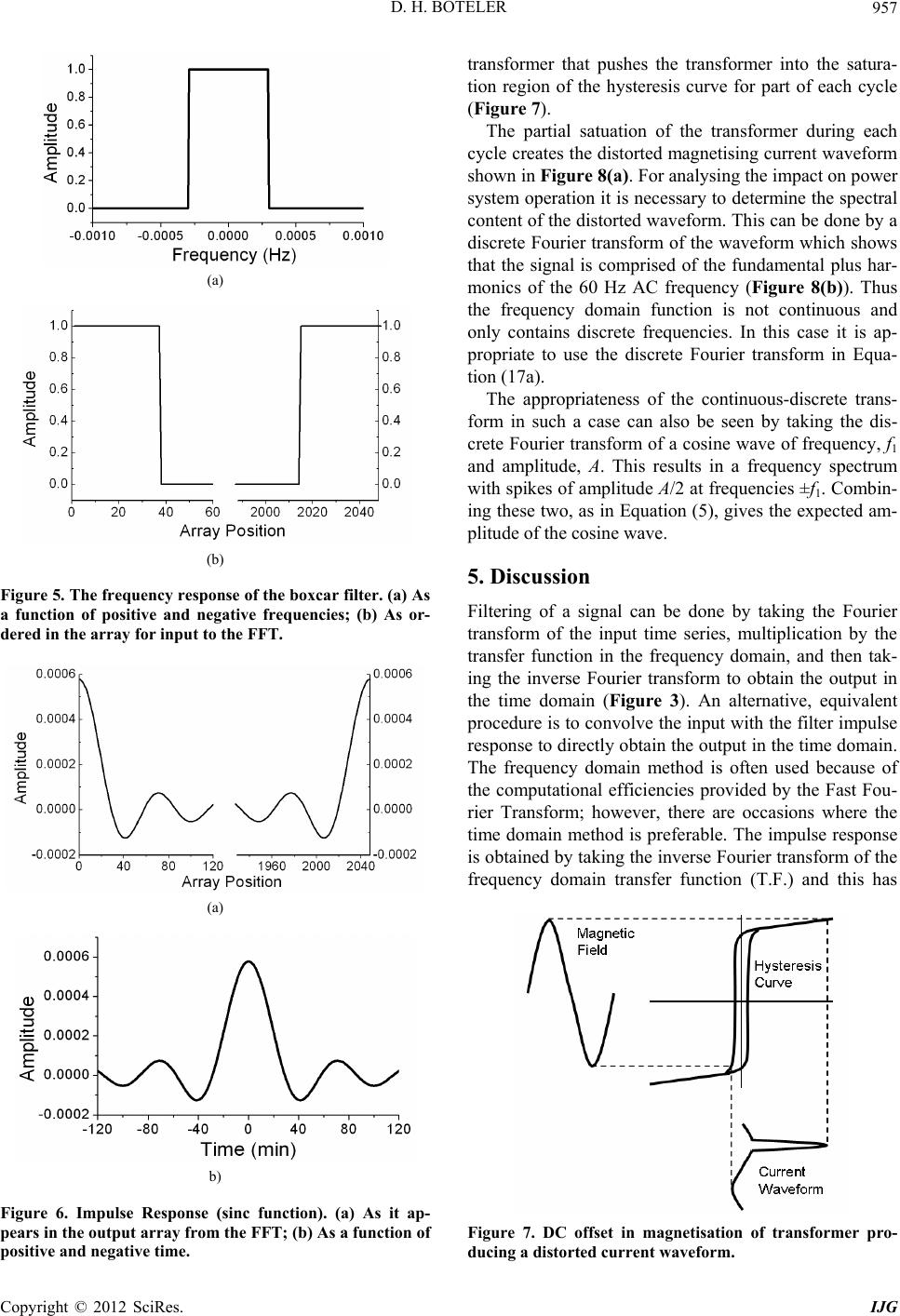

D. H. BOTELER 957
(a)
(b)
Figure 5. The frequency response of the boxcar filter. (a) As
a function of positive and negative frequencies; (b) As or-
dered in the array for input to the FFT.
(a)
Figure 6. Impulse Response (sinc function). (a) As it ap-
pears in the output array from the FFT; (b) As a function of
positive and negative time.
transformer that pushes the transformer into the satura-
tion region of the hysteresis curve for part of each cycle
(Figure 7).
The partial satuation of the transformer during each
cycle creates the distorted magnetising current waveform
shown in Figure 8(a). For analysing the impact on power
system operation it is necessary to determine the spectral
content of the distorted waveform. This can be done by a
discrete Fourier transform of the waveform which shows
that the signal is comprised of the fundamental plus har-
monics of the 60 Hz AC frequency (Figure 8(b)). Thus
the frequency domain function is not continuous and
only contains discrete frequencies. In this case it is ap-
propriate to use the discrete Fourier transform in Equa-
tion (17a).
The appropriateness of the continuous-discrete trans-
form in such a case can also be seen by taking the dis-
crete Fourier transform of a cosine wave of frequency, f1
and amplitude, A. This results in a frequency spectrum
with spikes of amplitude A/2 at frequencies ±f. Combin-
cted am-
plitude of the cosine wave.
5. Discussion
Filtering of a signal can be done by taking the Fourier
transform of the input time series, multiplication by the
transfer function in the frequency domain, and then tak-
ing the inverse Fourier transform to obtain the output in
the time domain (Figure 3). An alternative, equivalent
procedure is to convolve the input with the filter impulse
response to directly obtain the output in the time domain
The frequency domain me is often used because of
the computational efficiencies provided by the Fast Fou-
rier Transform; however, there are occasions where the
time domain method is preferable. The impulse response
is obtained by taking the inverse Fourier transform of the
frequency domain transfer function (T.F.) and this has
b)
1
ing these two, as in Equation (5), gives the expe
.
thod
Figure 7. DC offset in magnetisation of transformer pro-
ducing a distorted current waveform.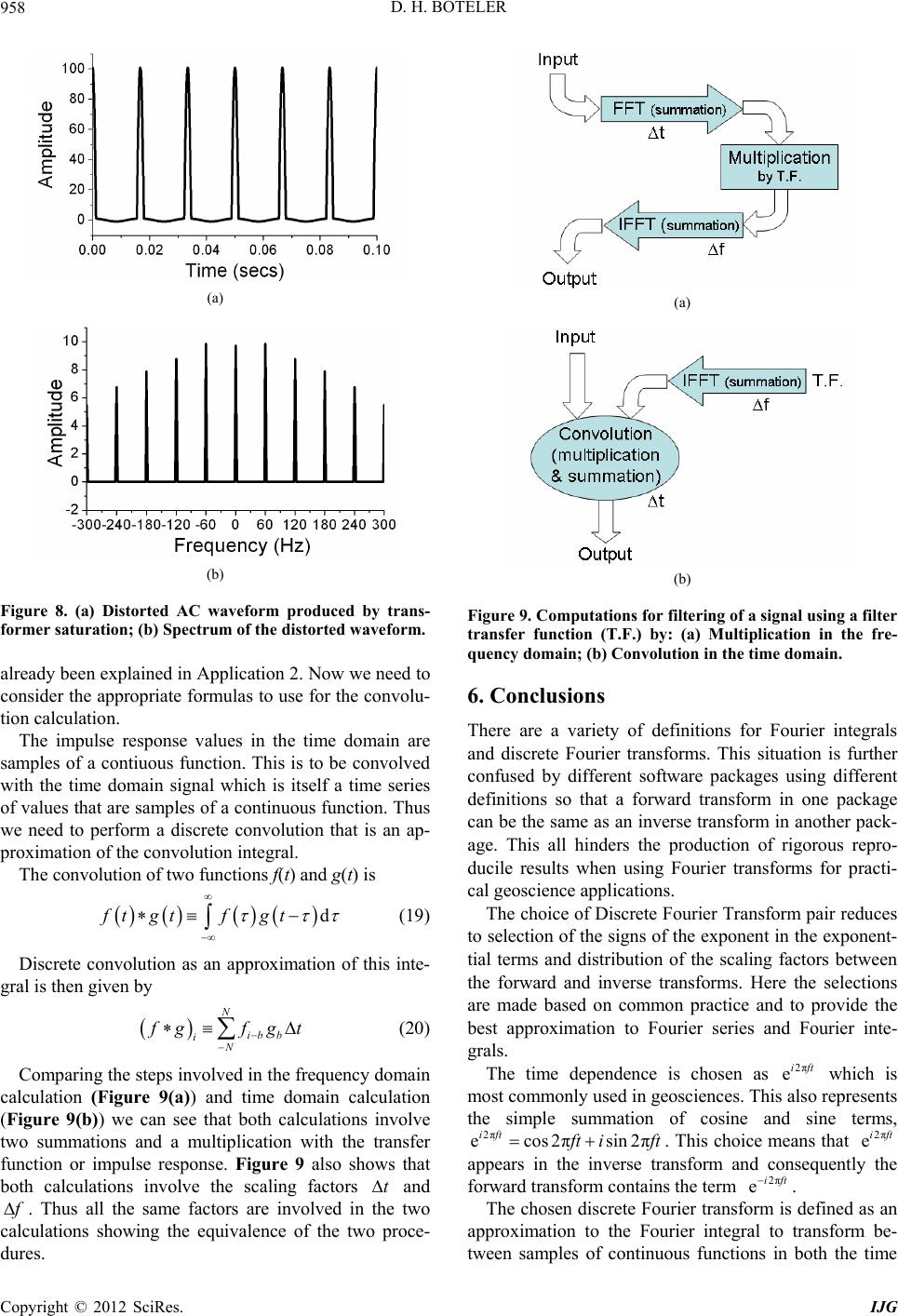

D. H. BOTELER 958
(a)
(b)
Figure 8. (a) Distorted AC waveform produced by trans-
former saturation; (b) Spectrum of the distorted waveform.
already been explained in Application 2. Now we need to
consider the appropriate formulas to use for the convolu-
tion calculation.
The impulse response values in the time domain are
samples of a contiuous function. This is to be convolved
with the time domain signal which is itself a time series
of values that are samples of a continuous function. Thus
we need to perform a discrete convolution that is an ap-
proximation of the convolution integral.
The convolution of two functions f(t) and g(t) is
 
dgt
 
ft gtf

  (19)
roximation of this inte-
gral is then given by
N
ib b
N




Discrete convolution as an app

i
f
gfgt



 (20)
Colved in the frequency domain
tions involve
two summations and a multiplication with the transfer
function or impulse response. Figure 9 also shows that
both calculations involve the scaling factors t

omparing the steps inv
calculation (Figure 9(a)) and time domain calculation
(Figure 9(b)) we can see that both calcula

and
f
. Thus all the same factors are involved in the two
calculations showing the equi of the two proce-
dures.
valence
(a)
uency domain; (b) Convolution in the time domain.
racti-
cal geoscience
The choice of Discrete Fourier Transform
to selection of the signs of the exponent in the exponent-
tia
rse transforms. Here the selections
are made based on common practice and to provide the
best approximation to Fourier series a
grals.
(b)
Figure 9. Computations for filtering of a signal using a filter
transfer function (T.F.) by: (a) Multiplication in the fre-
q
6. Conclusions
There are a variety of definitions for Fourier integrals
and discrete Fourier transforms. This situation is further
confused by different software packages using different
definitions so that a forward transform in one package
can be the same as an inverse transform in another pack-
age. This all hinders the production of rigorous repro-
ducile results when using Fourier transforms for p
applications.
pair reduces
l terms and distribution of the scaling factors between
the forward and inve
nd Fourier inte-
The time dependence is chosen as 2π eift which is
most commonly used in geosciences. This also represents
the simple summation of cosine and sine terms,
2π
ecos2πsin 2π
ift
f
ti ft . This choice means that 2π eift
appears in the inverse transform and consequently the
forward transform contains the term 2π eift.
he chosen discrete Fourier transform is defined as an
approximation to the Fourier integral to transform be-
tween s
T
amples of continuous functions in both the time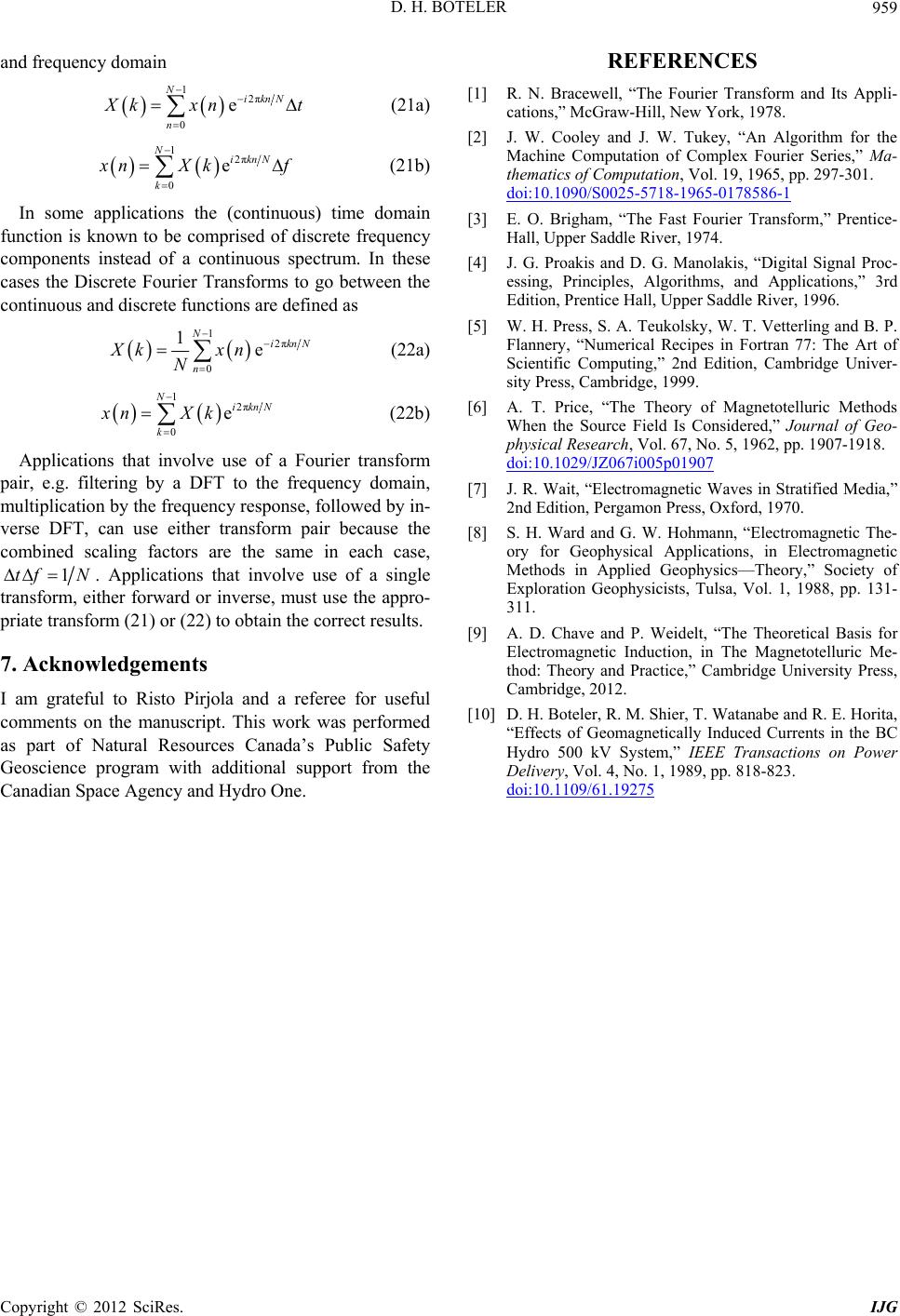

D. H. BOTELER 959
and frequency domain

1
0
N
n
2π
eik
nN
X
kx


n t


(21a)

1
0
N
k
2π
eik
nN
x
nX


k f (21b)
In some applications the (continuous) time domain
function is known to be comprised of discrete frequency
components instead of a continuous spectrum. In these
cases the Discrete Fourier Transforms to go betwe
continuous and discrete fun are defined as
en the
ctions
 
1
0
1N
n
Xk N


2π eik
nN
xn  (22a)

1
0
N
k
xn



Applications th
2π
eik
nN
X k (22b)
at involve use of a Fourier transform
pair, e.g. filtering by a DFT to the frequency domain,
multiplication by the frequency response, followed by in-
verse DFT, can use either transform pair because the
combined scaling factors are the same in each case,
1tfN. Applicationst involve use of a single
transform, either forward or inverse, must use the appro-
isto Pirjola and a referee for useful
ERENCES
[1] R. N. Bracewell, “The Fourier Transfo
cations,” McGraw-Hill, New York, 197
[2] J. W. Cooley and J. W. Tukey, “An Algorithm for the
Machine Computation of Complex F
thematics of Computation, Vol. 19, 19
doi:10.1090/S0025-5718-1965-0178586-1
REF
rm and Its Appli-
8.
ourier Series,” Ma-
65, pp. 297-301.
[3]
.
[5] W. H. Press, S. A. Teukolsky, W. T. Vetterling and B. P.
Flannery, “Numerical Recipes in Fortra
Scientific Computing,” 2nd Edition, Ca
sity Press, Cambridge, 1999.
[6] A. T. Price, “The Theory of M
When the Source Field Is Consid
physical Research, Vol. 67, No. 5, 1962, pp. 1907-1918.
E. O. Brigham, “The Fast Fourier Transform,” Prentice-
Hall, Upper Saddle River, 1974.
[4] J. G. Proakis and D. G. Manolakis, “Digital Signal Proc-
essing, Principles, Algorithms, and Applications,” 3rd
Edition, Prentice Hall, Upper Saddle River, 1996
n 77: The Art of
mbridge Univer-
agnetotelluric Methods
ered,” Journal of Geo-
doi:10.1029/JZ067i005p01907
[7] J. R. Wait, “Electromagnetic Waves in Stratified Media,”
2nd Edition, Pergamon Press, Oxford, 1970.
[8] S. H. Ward and G. W. Hohmann, “Electromagnetic The-
ory for Geophysical Applications, in Electromagnetic
s in Applied Geophysics—Theory,” Society of
Exploration Geophysicists, Tulsa, Vol. 1, 1988, pp. 131-
311.
[9] A. D. Chave and P. Weidelt, “The Theoretical Basis for
Method
, in The Magnetotelluric Me-
,” Cambridge University Press,
tha
priate transform (21) or (22) to obtain the correct results.
7. Acknowledgements Electromagnetic Induction
thod: Theory and Practice
Cambridge, 2012.
[10] D. H. Boteler, R. M. Shier, T. Watanabe and R. E. Horita,
“Effects of Geomagnetically Induced Currents in the BC
Hydro 500 kV System,” IEEE Transactions on Power
Delivery, Vol. 4, No. 1, 1989, pp. 818-823.
doi:10.1109/61.19275
I am grateful to R
comments on the manuscript. This work was performed
as part of Natural Resources Canada’s Public Safety
Geoscience program with additional support from the
Canadian Space Agency and Hydro One.