 Journal of Information Security, 2012, 3, 259-271 http://dx.doi.org/10.4236/jis.2012.34033 Published Online October 2012 (http://www.SciRP.org/journal/jis) Category-Based Intrusion Detection Using PCA Gholam Reza Zargar1, Tania Baghaie2 1GIS Department, Khuzestan Electrical Power Distributed Company, Ahvaz, Iran 2Training Center of Applied Science and Technology, Tehran Municipality Information and Communication Technology Organization, Tehran, Iran Email: zargar@vu.iust.ac.ir, baghaie@vu.iust.ac.ir Received June 16, 2011; revised August 22, 2012; accepted September 5, 2012 ABSTRACT Existing Intrusion Detection Systems (IDS) examine all the network features to detect intrusion or misuse patterns. In feature-based intrusion detection, some selected features may found to be redundant, useless or less important than the rest. This paper proposes a category-based selection of effective parameters for intrusion detection using Principal Components Analysis (PCA). In this paper, 32 basic features from TCP/IP header, and 116 derived features from TCP dump are selected in a network traffic dataset. Attacks are categorized in four groups, Denial of Service (DoS), Remote to User attack (R2L), Remote to User attack (U2R) and Probing attack. TCP dump from DARPA 1998 dataset is used in the experiments as the selected dataset. PCA method is used to determine an optimal feature set to make the detection process faster. Experimental results show that feature reduction can improve detection rate for the category-based de- tection approach while maintaining the detection accuracy within an acceptable range. In this paper KNN classification method is used for the classification of the attacks. Experimental results show that feature reduction will significantly speed up the train and the testing periods for identification of the intrusion attempts. Keywords: Intrusion Detection; Principal Components Analysis; Data Dimension Reduction; Feature Selection; Classification 1. Introduction Intrusion Detection Systems (IDS) is designed to com- plement other security measures based on attack preven- tion (firewalls, antivirus, etc.). Amparo Alonso-Betanzos et al. [1] say that “The aim of the IDS is to inform the system administrator of any suspicious activities and to recommend specific actions to prevent or stop the intru- sion”. Intrusion can be defined as an attempt to gain un- authorized access to network resources [2]. IDS is neces- sary for effective computer system protection. There are two approaches for intrusion detection, i.e. signature- based and anomaly-based intrusion detection. In signa- ture-based or misuse detection method, patterns of well known attacks are used to identify intrusions [3]. In ano- maly-based intrusion detection, network traffic is moni- tored and compared versus any deviation from the estab- lished normal usage patterns to determine whether the current state of the network is anomalous. An anomalous traffic can be flagged as intrusion attempt. Misuse detec- tion uses well defined patterns known as signatures of the attacks. Anomaly-based detection builds a normal profile and anomalous traffic is detected when the deviation from the normal model reaches a preset threshold [4]. Signature-based IDSs typically require human input to create attack signatures or to determine effective models for the normal behavior [4]. Feature selection ranking can be used in anomaly-based and signature-based intru- sion detection systems. Feature selection is an important issue in intrusion detection. The reason for it is due to the large number of features that should be monitored for the intrusion detection purpose. Elimination of useless or less relevant features will maintain accuracy of the detec- tion while speeding up its calculations. Therefore, any reduction in the number of features used for the detection will significantly improve the overall performance of the IDS. In cases where there are no useless features, con- centrating on the most important ones is expected to im- prove the execution speed of an IDS. This increase in the detection speed will not affect accuracy of the detection in a significant way. Incorrect selection of the features may not only reduce the speed of the operation but may also reduce detection accuracy [5]. This paper reports a work aimed on improving the in- trusion detection time using a category-based intrusion detection model. In Figure 1, network traffic in divided into six groups, normal, DoS, R2L, U2R, Probing and Undetermined Anomalous Behavior (UAB). The main goal in a Category-Based Intrusion Detection (CBID) is C opyright © 2012 SciRes. JIS  G. R. ZARGAR, T. BAGHAIE 260 Figure 1. Category-based separation of the network traffic. to reduce the amount of data that is less important with regard to the intrusion detection and to eliminate them. This approach has the benefit of reducing memory re- quirements for storage, reducing data transfer and pro- cessing time, and improving the detection rate [6]. IDS has to examine a very large audit data in a short period of time. Therefore, any reduction in the volume of data may save the processing time [7]. Considering certain attack categorizes, some features in the traffic data are more relevant than the rest for in- trusion detection. Feature reduction can be performed in several ways [7-10]. In this paper, the category-based approach is used to find the relevance between features extracted from the network traffic. This paper also proposes a method based on TCP/IP header parameters and derived features se- lected from TCP dump network traffic dataset. In the proposed approach, Principal Components Analysis (PCA) is used as a dimension reduction technique. KNN classi- fication method is used the detection of the intrusion at- tempts and results are reported. 2. Related Works In a reported work, Chakraborty [11] reports that the exis- tence of irrelevant and redundant features generally af- fects the performance of machine learning part of the work. Chakraborty Proves that proper selection of the feature set results in better classification performance. A. H. Sung et al. [8] have demonstrated that the elimina- tion of these unimportant and irrelevant features did not significantly reduced performance of the IDS. Chebrolu et al. [7], report that an important advantage for combining redundant and complementary classifiers is to increase robustness, accuracy and better overall generalization. Chebrolu et al. [7] have also identified important input features in building IDS that are compu- tationally efficient and effective. In their reported work, they have investigated performance of three feature se- lection algorithms, i.e. Bayesian networks (BN), Classi- fication and Regression Trees (CART) and an ensemble of BN and CART. Sung and Mukkamala [8], have explored SVM and Neural Networks to identify and categorize features with respect to their importance to detect specific kinds of attacks such as probing, DoS, Remote to Local (R2L), and User to Root (U2R). They have also demonstrated that elimination of these less important and irrelevant features did not reduce the performance of IDS signifi- cantly. Mukkamala et al. [12] have demonstrated that use of ensemble of classifiers gave the best accuracy for each category of attack patterns. In designing a classifier, their first step was to carefully construct different connectional models to achieve best generalization performance for the classifiers. Sung and Mukkamala [13] have analyzed data from a large network traffic since it causes a pro- hibitively high overhead and often becomes a major problem for the IDS. Chebrolu et al. [7] proposed CART-BN approach, where CART performed best for Normal, Probe and U2R and the ensemble approach worked best for R2L and DoS. Meanwhile, A. Abraham et al. [14] proved that en- semble of Decision Tree was suitable for Normal, LGP for Probe, DoS and R2L and Fuzzy classifier was good for R2L attacks. A. Abraham et al. [15] demonstrated the ability of their proposed Ensemble structure in modeling light-weight distributed IDS. 3. Data Reduction and Feature Selection Using PCA Principal Components Analysis (PCA) is a predominant linear dimensionality reduction technique, and it has been widely applied on datasets in many different scien- tific domains [16]. PCA allows us to compute a linear transformation that maps data from a high dimensional space to a lower dimensional space. The first principal components have the highest contribution to the variance in the original dataset. Therefore, the rest can be disre- garded with minimal loss of the information value during the dimension reduction process. Another method is to use their weights and transform data in to a new space with lower dimensions. The transformation works in the following way [17]: 11 121 21 222 12 12 ,, , N N MN M MM MN xx x xx xxx x xx x (1) Given a set of observations x1, x2, ···, xM are N × 1 vectors, where each observation is represented by a vec- tor of length N. Thus, the dataset is presented by matrix Equation (1). The mean value for each column is defined by the ex- pected value. This is explained in Equation (2). 1 1M i i x M (2) Once the mean value is subtracted from the data yields expression Equation (3). Copyright © 2012 SciRes. JIS  G. R. ZARGAR, T. BAGHAIE 261 ii x (3) C that is correlation compute from matrix 12 M A (N × M Matrix), Equation (4): 12 1M M n1 TT nn C M AA (4) Sampled N × N covariance matrix characterizes how data is scattered [18]. The eigenvalues of C: λ1 > λ2 > ··· > λN and the eigen- vectors of C: u1, u2, ···, uN have to be calculated. Since C is symmetric, u1, u2, ···, uN form a basis (i.e. any vector x or actually x can, can be written as a linear com- bination of the eigenvectors) Equation (5). 112 2 1 N Nii i xbubu bu bu (5) During the dimensionality reduction, only the terms corresponding to the K largest eigenvalues are mentioned in Equation (6) [19]. 1 ˆ K ii i where xbu KN (6) The representation of ˆ x T b into the basis u1, u2, ···, uK is thus . 12 K The linear transformation RN ⇒ RK by PCA that per- forms the dimensionality reduction is presented in Equa- tion (7). bb T 11 22 T T T KK bu bu xUxx 2 000 000 00.0 000 n bu (7) The new variables (i.e. bi’s) are uncorrelated. The co- variance matrix for the bi’s is presented in Equation (8). 1 T UCU (8) The covariance matrix represents only second order statistics among the vector values. Let n to be the dimensionality of the data. The covari- ance matrix is used to calculate UTCU that is a diagonal matrix. UTCU is sorted and rearranged in the form of 12 n so that the data exhibits maximum variance in y1, the next largest variance in y2 and so on, with minimum variance in yn [20,21]. 4. K-Nearest Neighbor Algorithm (KNN) The K-nearest neighbor (KNN) decision rule has been a ubiquitous classification tool with good scalability. Ex- perience has shown that the optimal choice of K is de- pendent on the data. This makes it difficult to tune the parameters for different applications. KNN classification algorithm tries to find the K near- est neighbors of x0 and uses a majority vote to determine the class label of x 0. Without any prior knowledge, the KNN classifier usually applies Euclidean distances as the distance metric [22]. KNN is an example of instance-based learning, in which the training data set is stored, so that, a classifica- tion for a new unclassified record may be found simply by comparing it to the most similar records in the train- ing set. The most common distance function is Euclidean dis- tance, which represents the usual manner in which hu- mans think of distance in the real world (8): 2 Euclidean ,ii i dxy xy (8) where x = x1, x2, ···, xm, and y = y1, y2, ···, ym represent the m attribute values of two records [23,24]. 5. Three Way Handshake The three-way handshake in Transmission Control Pro- tocol (also called the three message handshake) is a method used to establish and tear down network connec- tions. This handshaking technique is referred to as the 3-way handshake or as “SYN-SYN-ACK” (or more ac- curately SYN, SYN-ACK, ACK). The TCP handshaking mechanism is designed so that two computers attempting to communicate can negotiate the parameters of the net- work connection before beginning communication. This process is also designed so that both ends can initiate and negotiate separate connections at the same time. Below is a (very) simplified description of the TCP 3-way hand- shake process (Figure 2). Source sends a TCP Synchronize packet to destina- tion; Destination receives source’s SYN; Destination sends a Synchronize Acknowledgement packet; Figure 2. Three-way handshake. Copyright © 2012 SciRes. JIS  G. R. ZARGAR, T. BAGHAIE 262 Source re ; acket; ent messages are id cation between two computers ends, an ing dataset eatures are extracted from TCP/IP nting pa set represents a single flow of TC n this work are di at ar 7.1. Denial of Service (DoS) Attacks amount of re- ceives destination’s SYN-ACK; Source sends an Acknowledgement packet Destination receives an Acknowledgement p TCP connection is established. Synchronization and Acknowledgem entified by a bit inside the TCP header of the segment. TCP knows whether the network connection is opened, synchronized or established by using the Synchronization and Acknowledgement messages when establishing a network connection. When the communi other 3-way communication is performed to tear down the TCP connection. This setup and teardown of a TCP connection is part of the reason why TCP qualifies to be a reliable protocol [25]. 6. The Dataset Used in This Work The DARPA’98 dataset was used for the train in the reported work. The dataset provides around 4 giga- bytes of compressed TCP dump data [26] for 7 weeks of the network traffic [27]. This dataset can be processed into about 5 millions of connection records each about 100 bytes in size. Dataset contains payload of the packets transmitted between hosts inside and outside a simulated military base. BSM1 audit data from one UNIX Solaris host for some network sessions are also provided. DARPA 1998 TCP dump dataset [28] was preprocessed and label- ed using two class labels, e.g., normal and attack. 7. Pre-Processing In this work 32 basic f header protocols. These features are derived from TCP, IP, UDP and ICMP packet headers without inspecting the payload. The possible candidates for this feature category includes timestamp, source port, source IP, destination port, destination IP, flag, to name a few. In another data- set 116 derived features are selected from TCP dump net- work traffic dataset [28]. This dataset is intended to pro- vide a wide variety of features characterizing flows. This includes simple statistics about packet length and in- ter-packet timings, and information derived from the transport protocol (TCP) such as SYN and ACK counts. This information is extracted using all the packets trans- mitted in both directions as well as on each direction individually (server → client and client → server). Many packet statistics are derived directly by cou ckets, and packet header-sizes. A significant number of features (such as estimates of round-trip time, size of TCP segments, and the total number of retransmissions) are derived from the TCP headers. TCP trace [29] was used for this information. Each object within data P packets between client and server. All of the features that are extracted i splayed in Appendix 1, Table A.1. Wire-shark, Edit- cap and TCP trace softwares are used to analyze and minimize TCP dump files and extract features [30,31]. The dataset contains 13 different types of attacks th e broadly categorized into five groups such as DoS, U2R, R2L, Probing and anomalous behavior. Goal is categorize different intrusion methods into a number of categories. This approach aims to summarize the intru- sion method into a few similar approaches. Following the proposed approach, system will be able to deal with variations of the different attacks within each category. Considering the DARPA’98 dataset, there are five main categories of attacks proposed in this paper. The pro- posed attack categories are listed and described in the following sections. Denial of service attacks consume a large sources thus preventing legitimate users from receiving service with some minimum performance or they may prevent a computer from complying with a legitimate requests by consuming its resources [32,33]. Apache2, Back, Land, Mail bomb, SYN Flood, Ping of death, Process table, Smurf, Teardrop, Udpstorm and Neptune attacks are some examples of the Dos attack. In this work Syn flood attack is used for the experiments. Therefore, Syn flood scenario will be explained in this section: Syn flood is a DoS attack in which every TCP/IP implement- tation is vulnerable to it in some degree. Each half-open TCP connection made to a machine will cause the “tcpd” server to add a record to the data structure that stores information describing all pending connections (Figure 3). This data structure has a size limit and it may over- flow by intentionally creating too many partially-open connections. The half-open connections data structure on the victim server system will eventually fill up. Once the data structure is full, unless the table is emptied, the sys- tem will not be able to accept any new incoming con- Figure 3. Attacking a victim machine with half-open con nections. - 1Basic Security Monitoring (BSM). Copyright © 2012 SciRes. JIS 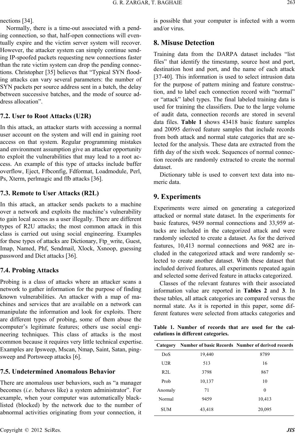 G. R. ZARGAR, T. BAGHAIE 263 nections [34]. Normally, th ing connection ere is a time-out associated with a pend- t Attacks (U2R) ccessing a normal s to a machine acks where an attacker scans a s Behavior manager etection ARPA dataset includes “list estamp, source host and port, ta. ents imed on generating a categorized tate dataset. In the experiments for th , so that, half-open connections will even- tually expire and the victim server system will recover. However, the attacker system can simply continue send- ing IP-spoofed packets requesting new connections faster than the rate victim system can drop the pending connec- tions. Christopher [35] believes that “Typical SYN flood- ing attacks can vary several parameters: the number of SYN packets per source address sent in a batch, the delay between successive batches, and the mode of source ad- dress allocation”. 7.2. User to Roo In this attack, an attacker starts with a user account on the system and will end in gaining root access on that system. Regular programming mistakes and environment assumption give an attacker opportunity to exploit the vulnerabilities that may lead to a root ac- cess. An example of this type of attacks include buffer overflow, Eject, Ffbconfig, Fdformat, Loadmodule, Perl, Ps, Xterm, perlmagic and ffb attacks [36]. 7.3. Remote to User Attacks (R2L) In this attack, an attacker sends packet over a network and exploits the machine’s vulnerability to gain local access as a user illegally. There are different types of R2U attacks; the most common attack in this class is carried out using social engineering. Examples for these types of attacks are Dictionary, Ftp_write, Guest, Imap, Named, Phf, Sendmail, Xlock, Xsnoop, guessing password and Dict attacks [36]. 7.4. Probing Attacks Probing is a class of att network to gather information for the purpose of finding known vulnerabilities. An attacker with a map of ma- chines and services that are available on a network can manipulate the information and look for exploits. There are different types of probing, some of them abuse the computer’s legitimate features; others use social engi- neering techniques. This class of attacks is the most common because it requires very little technical expertise. Examples are Ipsweep, Mscan, Nmap, Saint, Satan, ping- sweep and Portsweep attacks [6]. 7.5. Undetermined Anomalou There are anomalous user behaviors, such as “a becomes (i.e. behaves like) a system administrator”. For example, when your computer was automatically black- listed (blocked) by the network due to the number of abnormal activities originating from your connection, it is possible that your computer is infected with a worm and/or virus. 8. Misuse D Training data from the D files” that identify the tim destination host and port, and the name of each attack [37-40]. This information is used to select intrusion data for the purpose of pattern mining and feature construc- tion, and to label each connection record with “normal” or “attack” label types. The final labeled training data is used for training the classifiers. Due to the large volume of audit data, connection records are stored in several data files. Table 1 shows 43418 basic feature samples and 20095 derived feature samples that include records from both attack and normal state categories that are se- lected for the analysis. These data are extracted from the fifth day of the sixth week. Sequences of normal connec- tion records are randomly extracted to create the normal dataset. Dictionary table is used to convert text data into nu- meric da 9. Experim Experiments were a attacked or normal s basic features, 9459 normal connections and 33,959 at- tacks are included in the categorized attack and were randomly selected to create a dataset. As for the derived features, 10,413 normal connections and 9682 are in- cluded in the categorized attack and were randomly se- lected to create another dataset. With these dataset that included derived features, all experiments repeated again and selected some derived feature in attacks categorized. Classes of the relevant features with their associated information value are reported in Tables 2 and 3. In ese tables, all attack categories are compared versus the normal state. As it is reported in this paper, some dif- ferent features were selected from attacks categories and Table 1. Number of records that are used for the cal- culations in different categories. CategoryNumber of basic Records Number of derived records DoS 19,440 8789 U2R 513 16 R2L 3798 867 Prob 1 A y N1 20, 0,13710 nomal71 0 ormal9459 0,413 SUM 43,418 095 Copyright © 2012 SciRes. JIS 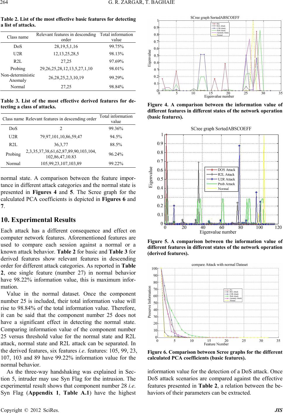 G. R. ZARGAR, T. BAGHAIE 264 Tist of the most effective basic featuetecting a list of Relevant features in descending ation able 2. L attacks. res for d Class name order value Total inform DoS 28,19,5,1,16 99.75% U2R R2L 12,13,25,28,5 27,25 98.13% 7.69%9 P 29,26,21,10 Non-d A26,9 99. robing5,28,12,13,5,27,98.01% eterministic nomaly 28,10,125,2,3,29% Normal 27,25 98.84% most effective deriv Figure 4. A comparison between the information value of different features in different states of the network operation (basic features). Tabt of the ed feat de- tectss of attacks. Total information le 3. Lisures for ing a cla Class name Relevant features in descending order value DoS 2 99.36% U2R 79,97,101,10,86,59,47 94.5% 88.5% R2L 36,3, 2,8 77 P 2,3,35,37,38,61,67,89,90,103,104, N 105,9903,89 robing 102,86,47,10.83 96.24% ormal,23,107,199.22% noate. A coeen the feapor- tance in differennd the note is presented in Figures 4 and. The Scree graph for the h attack has a different consequence and effect on ementioned features are against a normal or a .84% of the total information value. Therefore, it t shows that component number 28 i.e. Sy rmal stmparison betwture im t attack categories armal sta 5 calculated PCA coefficients is depicted in Figures 6 and 7. 10. Experimental Results Eac computer network features. Afor used to compare each session known attack behavior. Table 2 for basic and Table 3 for derived features show relevant features in descending order for different attack categories. As reported in Table 2, one single feature (number 27) in normal behavior have 98.22% information value, this is maximum infor- mation. Value in the normal dataset. Once the component number 25 is included, their total information value will rise to 98 can be said that the component number 25 does not have a significant effect in detecting the normal state. Comparing information value of the component number 25 versus threshold value for the normal state and R2L attack, normal state and R2L attack can be separated. In the derived features, six features i.e. features: 105, 99, 23, 107, 103 and 89 have 99.22% information value for the normal behavior. As the three-way handshaking was explained in Sec- tion 5, intruder may use Syn Flag for the intrusion. The experimental resul n Flag (Appendix 1, Table A.1) have the highest Figure 5. A comparison between the information value of different features in different states of the network operation (derived features). Figure 6. Comparison between Scree graphs for the different calculated PCA coefficients (basic features). t the effective features presented in Table , a relation between the be- information value for the detection of a DoS attack. Once DoS attack scenarios are compared agains 2 haviors of their parameters can be extracted. Copyright © 2012 SciRes. JIS 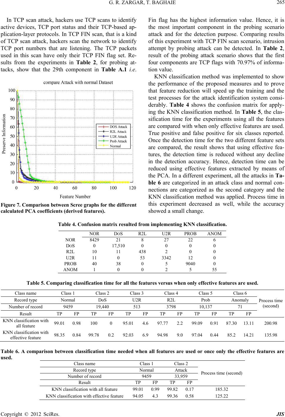 G. R. ZARGAR, T. BAGHAIE Copyright © 2012 SciRes. JIS 265 at is a kind of In TCP scan attack, hackers use TCP scans to identify active devices, TCP port status and their TCP-based ap- plication-layer protocols. In TCP FIN scan, th Fin flag has the highest information value. Hence, it is the most important component in the probing scenario attack and for the detection purpose. Comparing results of this experiment with TCP FIN scan scenario, intrusion attempt by probing attack can be detected. In Table 2, result of the probing attack scenario shows that the first four components are TCP flags with 70.97% of informa- tion value. TCP scan attack, hackers scan the network to identify TCP port numbers that are listening. The TCP packets used in this scan have only their TCP FIN flag set. Re- sults from the experiments in Table 2, for probing at- tacks, show that the 29th component in Table A.1 i.e. Figure 7. Comparison between Scree graphs for the different calculated PCA coefficients (derived features). om implementing KNN classification. DOS R2L U2R PROB ANOM KNN classification method was implemented to show the performance of the proposed measures and to prove that feature reduction will speed up the training and the test processes for the attack identification system consi- derably. Table 4 shows the confusion matrix for apply- ing the KNN classification method. In Table 5, the clas- sification time for the experiments using all the features are compared with when only effective features are used. True positive and false positive for six classes reported. Once the detection time for the two different feature sets are compared, the result shows that using effective fea- tures, the detection time is reduced without any decline in the detection accuracy. Hence, detection time can be reduced using effective features extracted by means of the PCA. In a different experiment, all the attacks in Ta- ble 6 are categorized in an attack class and normal con- nections are categorized as the second category and the KNN classification method was applied. Process time in this experiment decreased as well, while the accuracy showed a small change. Table 4. Confusion matrix resulted fr NOR NOR 8429 21 8 27 22 6 DOS 0 17,510 0 0 0 0 R2L 10 9 ANOM 11 0 438 53 2 3342 0 12 0 0 U PROB 2R11 40 38 0 5 040 0 1 0 0 2 5 55 Table 5. Compasificn timeall the features ve whenfectifeatures are used. Class name Class 2 Classss 4 Class 5Class 6 ring clasatio for rssu only efve lass 1 C 3 Cla Record type Normal DoS U2R R2L Prob Anomaly Number of record 9459 19,440 513 3798 10,137 71 TP FP TP FP TP FP TP FP TP FP TP FP rocess time (second) P Result KNNwith 99. 1000 95.06 97.72 99.0.91 871 classification all feature 01 0.98 14.72.90.30 13.1200.98 KNN clith 9 9 9991 135.98 assificati ctive feat on w effeure 8.350.84 9.780.2 2.036.9 4.989.0 7.040.44 85.2 4.21 T between classification time needed when all features are used or once only the effective features are use Class name Class 1 Class 2 able 6. A comparison d. Record type Normal Attack Number of record 9459 33,959 Process time (second) Result TP FP T P FP KNN classification with all feature 99999. 7.01 0.9820.1185.32 KNN classification with effective feature 94.05 4.3 99.360.58125.22  G. R. ZARGAR, T. BAGHAIE 266 11. Conclusions A feature selection momp nent Analysis (PCpl esults with a similar accuracy f features. The proposed approac tri s to detect intrusions. Using the results derived ction and comparing it versus both d feature sets, one can analyze the elia, M. C.-F. Félix, A. S. Classification of Computer In- trusions Using Functional Networks—A Comparative Study,” Proceeosium on Artifi [3] K. Ilgun, R. A. Kemmerer and P. A. Porras, “State Tra sition is: A Rule-Based Intrusion Detection Ap- proach,” IEEE Transaction on Software Engineering, Vol. 21, No. 3, 1995, pp. 181-:10.1109/32.372146 ethod based on Principal Co- A) for CBID is proposed and ime- mented to provide r with a smaller set o but h improved the detection speed. Feature selection reduced the total number of features in the dataset (32 basic fea- tures and 116 derived features). Due to the smaller search space, this reduction means that less data is needed for training the classifier. Paper reports a new CBID ap- proach that can produce better and more accurate results in identifying the category of the attacks instead of the precise type of the attack. This result also indicates that there are analytical solutions for the feature selection that are not based on the trial and error. The possibility and feasibility of detecting intrusions based on characteriza- tion of different types of attacks such as DoS, probes, U2R and R2L attacks is an important goal in the reported work. Results of this investigation seem to be promising. Results indicate that normal state of the network and category of the attacks can be identified using a small number of a carefully selected network features. On the other hand, it is proven that certain features have no con- bution to intrusion detection. Experimental results show that dimension reduction and identification of effective network features for category-based selection can reduce the process time in an intrusion detection system while maintaining the detection accuracy within an acceptable range. 12. Future Work Plan for the future work is to use different classification method from the intrusion dete the full and the reduce differences in their accuracy and speed. Also merging KDD Cup 99 features with 116 newly derived features to generate one single dataset and repeat all the experiment for the new dataset and to compare the result with the result reported in this paper. REFERENCES [1] A.-B. Amparo, S.-M. No Juan and P.-S. Beatriz, “ -R. dings of European Sympcial Neural Networks (ESANN), Bruges, 25-27 April 2007, pp. 579- 584. [2] R. Heady, G. Luger, A. Maccabe and M. Servilla, “The Architecture of a Network Level Intrusion Detection Sys- tem,” Technical Report, University of New Mexico, Al- buquerque, 1990. n- Analys 199. doi [4 I. and A. ElisseeIntroduction to Variable Using Feature Selection of Soft Com- ed- ] Guyonff, “An and Feature Selection,” Journal of Machine Learning Re- search, Vol. 3, 2003, pp. 1157-1182. [5] T. S. Chou, K. K. Yen and J. Luo, “Network Intrusion Detection Design puting Paradigms,” International Journal of Computa- tional Intelligence, Vol. 4, No. 3, 2008, pp. 196-208. [6] G. Zargar and P. Kabiri, “Identification of Effective Net- work Feature for Probing Attack Detection,” Proce ings of 1st International Conference on Network Digital Technologies, July 2009, pp. 405-410. doi:10.1109/NDT.2009.5272124 [7] S. Chebrolu, A. Abraham and J. Thomas, “Feature De- duction and Ensemble Design of Intrusion Detection Systems,” Computers and Security, Elsevier Science, Vol. 24, No. 4, 2005, pp. 295-307. [8] A. H. Sung and S. Mukkamala, “Identifying Important Features for Intrusion Detection Using Support Vector Machines and Neural Networks,” Proceedings of Inter- national Symposium on Applications and the Internet (SAINT), 2003, pp. 209-216. [9] R. Agrawal, J. Gehrke, D. Gunopulos and P. Raghavan, “Automatic Subspace Clustering of High Dimensional Data for Data Mining applications,” Proceedings of Acm- sigmod International Conference on Management of Data, Seattle, 1998, pp. 94-105. [10] M. F. Abdollah, A. H. Yaacob, S. Sahib, I. Mohamad and M. F. Iskandar, “Revealing the Influence of Feature Se- lection for Fast Attack Detection,” International Journal of Computer Science and Network Security, Vol. 8, No. 8, 2008, pp. 107-115. [11] B. Chakraborty, “Feature Subset Selection by Neuro-Rough Hybridization,” Lecture Notes in Computer Science (LNCS), Springer, Hiedelberg, 2005. [12] S. Mukkamala, A. H. Sung and A. Abraham, “Modeling ction Problems,” Lecture Notes in Systems,” Springer, Hiedel- . 3, 2007, pp. 1890.1401903 Intrusion Detection Systems Using Linear Genetic Pro- gramming Approach,” Lecture Notes in Computer Sci- ence (LNCS), Springer, Hiedelberg, 2004. [13] A. H. Sung, and S. Mukkamala, “The Feature Selection and Intrusion Dete Computer Science (LNCS), Springer, Hieldelberg, 2004. [14] A. Abraham and R. Jain, “Soft Computing Models for Network Intrusion Detection berg, 2004. [15] A. Abraham, C. Grosan and C. M. Vide, “Evolutionary Design of Intrusion Detection Programs,” International Journal of Network Security, Vol. 4, No 328-339. [16] C. Boutsidis, M. W. Mahoney and P. Drineas, “Unsu- pervised Feature Selection for Principal Components Analysis,” Proceedings of the 14th ACM Sigkdd Interna- tional Conference on Knowledge Discovery and Data Mining, Las Vegas, 2008, pp. 61-69. doi:10.1145/140 [17] W. Wang and R. Battiti, “Identifying Intrusions in Com- Copyright © 2012 SciRes. JIS 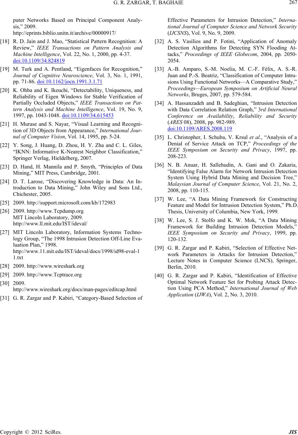 G. R. ZARGAR, T. BAGHAIE 267 puter Networks Based on Principal Component Analy- sis,” 2009. http://eprints.biblio.unitn.it/archive/00000917/ [18] R. D. Jain and J. Mao, “Statistical Pattern Recognition: A Review,” IEEE Transactions on Pattern Analysis and Machine Intelligence, Vol. 22, No. 1, 2000, pp. 4-37. doi:10.1109/34.824819 [19] M. Turk and A. Pentland, “Eigenfaces Journal of Cognitive Neuroscie for Recognition, nce, Vol. 3, No. 1, 1991 ” , pp. 71-86. doi:10.1162/jocn.1991.3.1.71 [20] K. Ohba and K. Ikeuchi, “Detectability, Uniqueness, and Reliability of Eigen Windows for Stable Veri Partially Occluded Objects,” IEEE Transaction fication of s o n Pat- tern Analysis and Machine Intelligence, Vol. 19, No. 9, 1997, pp. 1043-1048. doi:10.1109/34.615453 [21] H. Murase and S. Nayar, “Visual Learning and Reco tion of 3D Objects from gni- Appearance,” International Jour- Classification,” n-pages/editcap.html on Detection,” Interna- ournal of Computer Science and Network Security Networks, Bruges, 2007, pp. 579-584. [34] A. Hassanzadeh and B. Sadeghian, “Intrusion Detection with Data Correlation Relation Graph,” 3rd International Conference on Availability, Reliability and Security (ARES 08), 2008, pp. 982-989. nal of Computer Vision, Vol. 14, 1995, pp. 5-24. [22] Y. Song, J. Huang, D. Zhou, H. Y. Zha and C. L. Giles, “IKNN: Informative K-Nearest Neighbor Springer Verlag, Hieldelberg, 2007. [23] D. Hand, H. Mannila and P. Smyth, “Principles of Data Mining,” MIT Press, Cambridge, 2001. [24] D. T. Larose, “Discovering Knowledge in Data: An In- troduction to Data Mining,” John Wiley and Sons Ltd., Chichester, 2005. [25] 2009. http://support.microsoft.com/kb/172983 [26] 2009. http://www.Tcpdump.org MIT Lincoln Laboratory, 2009. http://www.ll.mit.edu/IST/ideval/ [27] MIT Lincoln Laboratory, Information Systems Techno- logy Group, “The 1998 Intrusion Detection Off-Line Eva- luation Plan,” 1998. http://www.11.mit.edu/IST/ideval/docs/1998/id98-eval-1 1.txt [28] 2009. http://www.wireshark.org [29] 2009. http://www.Tcptrace.org [30] 2009. http://www.wireshark.org/docs/ma [31] G. R. Zargar and P. Kabiri, “Category-Based Selection of Effective Parameters for Intrusi tional J (IJCSNS), Vol. 9, No. 9, 2009. [32] A. S. Vasilios and P. Fotini, “Application of Anomaly Detection Algorithms for Detecting SYN Flooding At- tacks,” Proceedings of IEEE Globecom, 2004, pp. 2050- 2054. [33] A.-B. Amparo, S.-M. Noelia, M. C.-F. Félix, A. S.-R. Juan and P.-S. Beatriz, “Classification of Computer Intru- sions Using Functional Networks—A Comparative Study,” Proceedings—European Symposium on Artificial Neural doi:10.1109/ARES.2008.119 [35] L. Christopher, I. Schuba, V. Krsul et al., “Analysis of a Denial of Service Attack on TCP,” Proceedings of the IEEE Symposium on Security and Privacy, 1997, pp. 208-223. [36] N. B. Anuar, H. Sallehudin, A. Gani and O. Zakaria, “Identifying False Alarm for Network Intrusion Detection System Using Hybrid Data Mining and Decision Tree,” Malaysian Journal of Computer Science, Vol. 21, No. 2, 2008, pp. 110-115. [37] W. Lee, “A Data Mining Framework for Constructing Feature and Model for Intrusion Detection System,” Ph.D. Thesis, University of Columbia, New York, 1999. [38] W. Lee, S. J. Stolfo and K. W. Mok, “A Data Mining Framework for Building Intrusion Detection Models,” IEEE Symposium on Security and Privacy, 1999, pp. 120-132. [39] G. R. Zargar and P. Kabiri, “Selection of Effective Net- work Parameters in Attacks for Intrusion Detection,” Lecture Notes in Computer Science (LNCS), Springer, Berlin, 2010. [40] G. R. Zargar and P. Kabiri, “Identification of Effective Optimal Network Feature Set for Probing Attack Detec- tion Using PCA Method,” International Journal of Web Application (IJWA), Vol. 2, No. 3, 2010. Copyright © 2012 SciRes. JIS 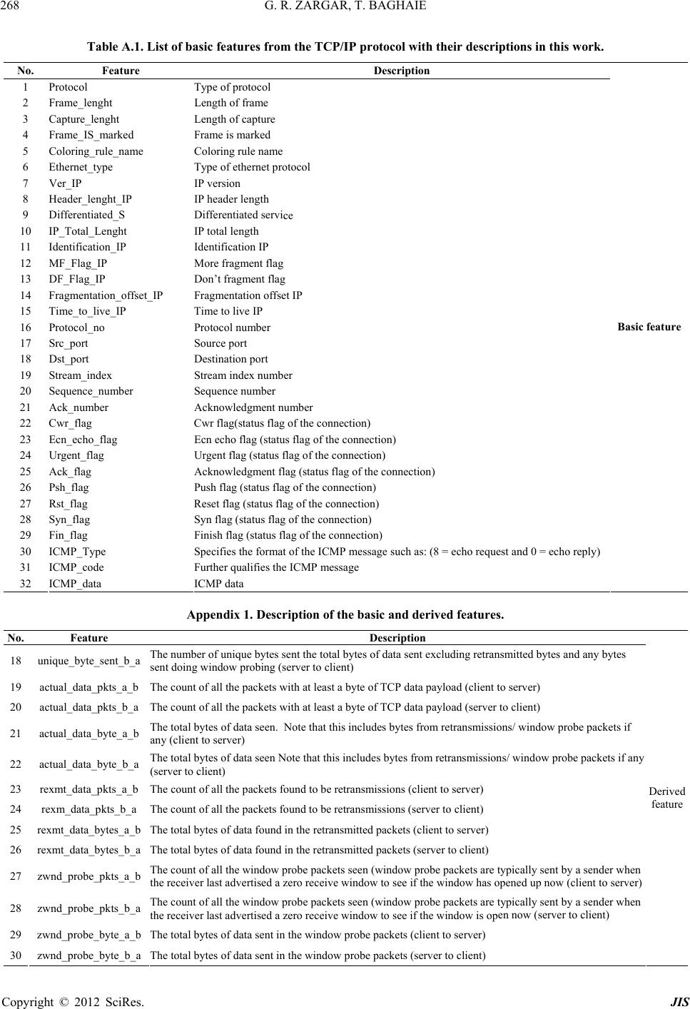 G. R. ZARGAR, T. BAGHAIE 268 Table A.1. List of basic features from the TCP/IP protocol with their descriptions in this work. No. Feature Description 1 Protocol Type of protocol 2 Frame_lenght Length of frame 3 Capture_lenght Length of capture 4 Frame_ Coloring_rule_Coloring rule name rotocol P ce et_IP set IP number the connection) _flag nection) of the connection) (status flag of the connection) n) = echo request and 0 = echo reply) e a Basic feature IS_marked Frame is marked 5 6 name pe Ethernet_ty Ver_IP Type of ethernet p IP version 7 8 Header_lenght_I Differentiated_S IP header length 9 IP_Total_Lenght Differentiated servi 10 IP total length 11 Identification_IP Identification IP 12 MF_Flag_IP More fragment flag 13 DF_Flag_IP Fragmentation_offs Don’t fragment flag Fragmentation off14 15 Time_to_live_IP Time to live IP 16 Protocol_no Protocol number 17 Src_port Source port 18 Dst_port Destination port 19 Stream_indexStream index number 20 Sequence_number Sequence number 21 Ack_number Acknowledgment 22 Cwr_flag Cwr flag(status flag of 23 Ecn_echoEcn echo flag (status flag of the con Urgent flag (statu24 Urgent_flag Ack_flag s flag Acknowledgment flag 25 26 Psh_flag Push flag (status flag of the connectio 27 Rst_flag Reset flag (status flag of the connection) Syn flag (status flag of the connection) 28 Syn_flag 29 Fin_flag Finish flag (status flag of the connection) 30 ICMP_Type Specifies the format of the ICMP message such as: (8 Further qualifies the ICMP message 31 ICMP_cod 32 ICMP_datICMP data Ac and derived features. N ppendix 1. Description of the basi Description Feature o. The numf data sent excluding retransmitted bytes and any bytes sent doin unnt_b_a 1ber of unique bytes sent the total bytes o obing (server to client) g window pr ique_byte_se8 The count of all the packets with at least a byte of TCP data payload (client to server) actual_data_pkts_a_b 19 The couclient) actual_data_pkts_b_a 20 The total bytes of data seen. Note that this incl retransmissions/ window probe packets if actual_a_b udes bytes from retransmissions/ window probe packets if any actual_data_byte_b_a 22 rexm_data_pkts_b_a 24 found in the retransmitted packets (client to server) pically sent by a sender when opened up now (client to server) e typically sent by a sender when en now (server to client) zwnd_pr Derived feature The total bytes of data sent in the window probe packets (server to client) zwnd_probe_byte_b_a 30 nt of all the packets with at least a byte of TCP data payload (server to udes bytes from any (client to server) The total bytes of data seen Note that this incl _data_byte21 (server to client) The count of all the packets found to be retransmissions (client to server) rexmt_data_pkts_a_b 23 The count of all the packets found to be retransmissions (server to client) The total bytes of data rexmt_data_bytes_a_b 25 The total bytes of data found in the retransmitted packets (server to client) The count of all th rexmt_data_bytes_b_a 26 e window probe packets seen (window probe packets are ty the receiver last advertised a zero receive window to see if the window has zwnd_probe_pkts_a_b 27 The count of all the window probe packets seen (window probe packets ar the receiver last advertised a zero receive window to see if the window is op obe_pkts_b_a 28 The total bytes of data sent in the window probe packets (client to server) zwnd_probe_byte_a_b 29 Copyright © 2012 SciRes. JIS 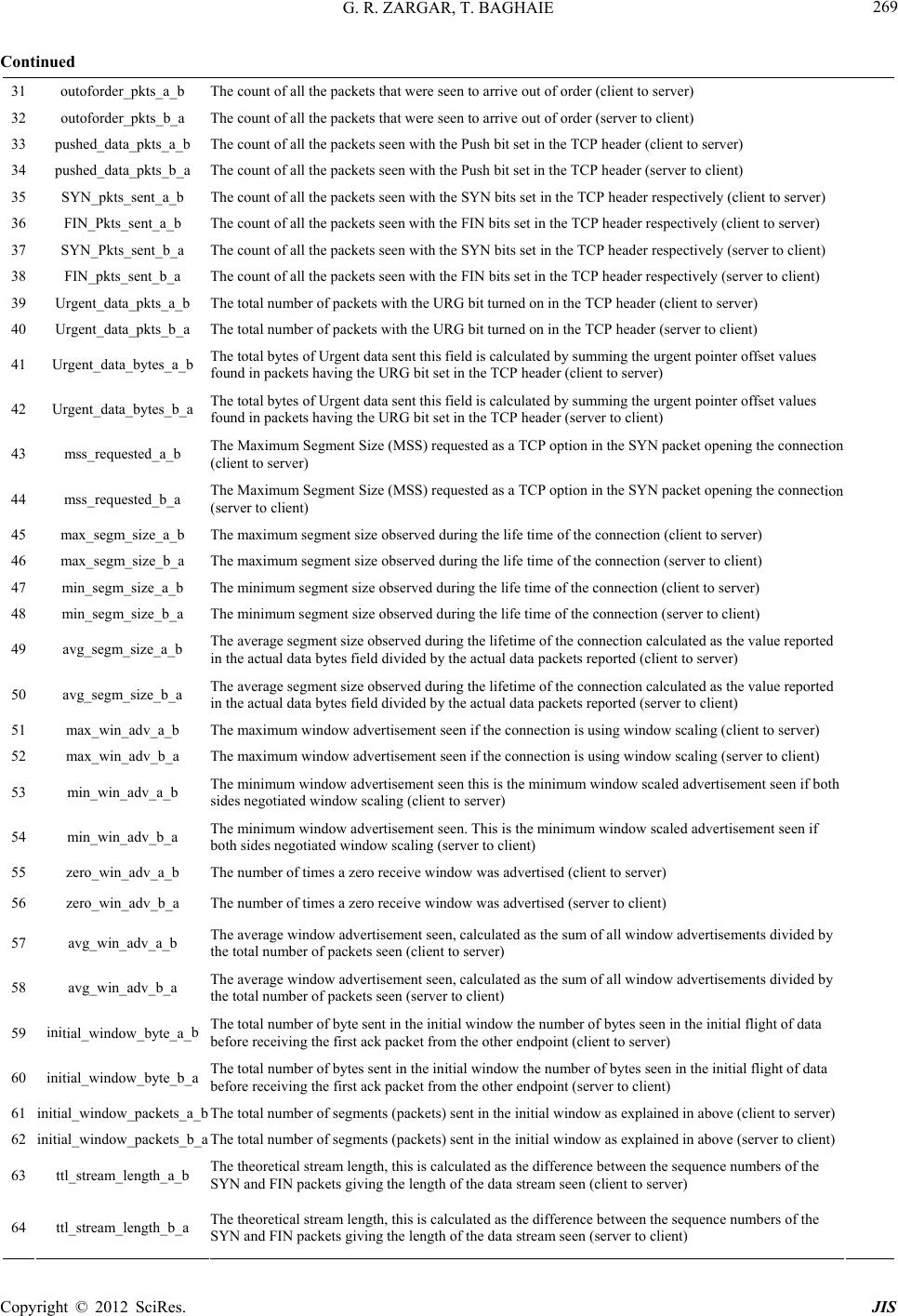 G. R. ZARGAR, T. BAGHAIE 269 Continue outoforder_pkts_a_b 31 d The count of all the packets that were seen to arrive out of order (client to server) The count of all the packets that were seen to arrive out of order (server to client) outoforder_pkts_b_a 32 The count of all the packets seen with the Push bit set in the TCP header (client to server) (server to client) The count of all the packets seen with the SYN bits set in the TCP header respectively (client to server) _pkts_sent_a_b ly (client to server) ely (server to client) er to client) ) U Ur e connection ion erver to client) ent size observed during the life time of the connection (server to client) min_segm_size_b_a 48 ytes field divided by the actual data packets reported (client to server) ue reported ver) inib ini_a initial_window_packets_a_b 61 initial window as explained in above (server to client)initial_window_pa r) pushed_data_pkts_a_b33 The count of all the packets seen with the Push bit set in the TCP header pushed_data_pkts_b_a34 SYN35 The count of all the packets seen with the FIN bits set in the TCP header respectiveFIN_Pkts_sent_a_b 36 The count of all the packets seen with the SYN bits set in the TCP header respectivSYN_Pkts_sent_b_a 37 The count of all the packets seen with the FIN bits set in the TCP header respectively (servFIN_pkts_sent_b_a 38 The total number of packets with the URG bit turned on in the TCP header (client to serverUrgent_data_pkts_a_b 39 The total number of packets with the URG bit turned on in the TCP header (server to client) Urgent_data_pkts_b_a 40 The total bytes of Urgent data sent this field is calculated by summing the urgent pointer offset values found in packets having the URG bit set in the TCP header (client to server) rgent_data_bytes_a_b41 The total bytes of Urgent data sent this field is calculated by summing the urgent pointer offset values found in packets having the URG bit set in the TCP header (server to client) gent_data_bytes_b_a42 The Maximum Segment Size (MSS) requested as a TCP option in the SYN packet opening th (client to server) mss_requested_a_b 43 The Maximum Segment Size (MSS) requested as a TCP option in the SYN packet opening the connect (server to client) mss_requested_b_a 44 The maximum segment size observed during the life time of the connection (client to server) The maximum segment size observed during the life time of the connection (s max_segm_size_a_b max_segm_size_b_a 45 46 The minimum segment size observed during the life time of the connection (client to server) The minimum segm min_segm_size_a_b 47 The average segment size observed during the lifetime of the connection calculated as the value reported in the actual data b avg_segm_size_a_b 49 The average segment size observed during the lifetime of the connection calculated as the val in the actual data bytes field divided by the actual data packets reported (server to client) avg_segm_size_b_a 50 The maximum window advertisement seen if the connection is using window scaling (client to sermax_win_adv_a_b 51 The maximum window advertisement seen if the connection is using window scaling (server to client)max_win_adv_b_a 52 The minimum window advertisement seen this is the minimum window scaled advertisement seen if both sides negotiated window scaling (client to server) min_win_adv_a_b 53 The minimum window advertisement seen. This is the minimum window scaled advertisement seen if both sides negotiated window scaling (server to client) min_win_adv_b_a 54 The number of times a zero receive window was advertised (client to server) zero_win_adv_a_b 55 The number of times a zero receive window was advertised (server to client) zero_win_adv_b_a 56 The average window advertisement seen, calculated as the sum of all window advertisements divided by the total number of packets seen (client to server) avg_win_adv_a_b 57 The average window advertisement seen, calculated as the sum of all window advertisements divided by the total number of packets seen (server to client) avg_win_adv_b_a 58 The total number of byte sent in the initial window the number of bytes seen in the initial flight of data before receiving the first ack packet from the other endpoint (client to server) tial_window_byte_a_59 The total number of bytes sent in the initial window the number of bytes seen in the initial flight of data before receiving the first ack packet from the other endpoint (server to client) tial_window_byte_b60 The total number of segments (packets) sent in the initial window as explained in above (client to server) The total number of segments (packets) sent in the ckets_b_a 62 The theoretical stream length, this is calculated as the difference between the sequence numbers of the SYN and FIN packets giving the length of the data stream seen (client to serve ttl_stream_length_a_b 63 The theoretical stream length, this is calculated as the difference between the sequence numbers of the SYN and FIN packets giving the length of the data stream seen (server to client) ttl_stream_length_b_a 64 Copyright © 2012 SciRes. JIS 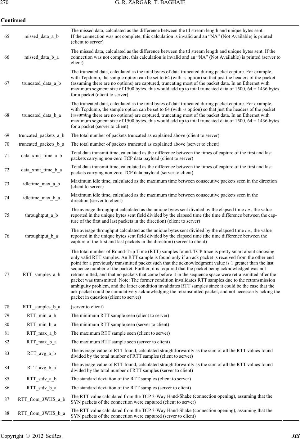 G. R. ZARGAR, T. BAGHAIE 270 C missed_data_a_b 65 ontinued The missed data, calculated as the difference between the ttl stream length and unique bytes sent. If the connection was not complete, this calculation is invalid and an “NA” (Not Available) is printed (client to server) The missed data, calculated as the difference between the ttl stream length and unique bytes sent. If the to The truncated data, calculated as the total bytes of data truncated during packet capture. For example, with Tcpdump, the sample option can be set to 64 (with -s option) so that just the headers of the packet h t to server) truncated_data_a_b 67 ng there are no options) are captured, truncating most of the packet data. In an Ethernet with tes truncated_data_b_a 68 t truncated_packets_b_a 70 data_xmit_time_a_b 71 maximum time between consecutive packets seen in the direction idletime_max_a_b 73 ackets seen in the me (the time difference between the cap- throughtput_a_b 75 t and last packets in the direction) (server to client) osing n RTT sample is found only if an ack packet is received from the other end ce space were retransmitted after the the RTT_samples_a_b 77 RTT_samples_b_a 78 RTT_min_a_b 79 RTT_max_a_b 81 RTT_max_b_a 82 culated straightforwardly as the sum of all the RTT values found mber of RTT samples (client to server) RTT_avg_a_b 83 rwardly as the sum of all the RTT values found r to client) to server) to client) nd-Shake (connection opening), assuming that the RTT onnection opening), assuming that the SYN packets of the connection were captured (server to client) RTT_from_3WHS_b_a 88 connection was not complete, this calculation is invalid and an “NA” (Not Available) is printed (server client) missed_data_b_a 66 (assuming there are no options) are captured, truncating most of the packet data. In an Ethernet wit maximum segment size of 1500 bytes, this would add up to total truncated data of 1500, 64 = 1436 bytes for a packet (clien The truncated data, calculated as the total bytes of data truncated during packet capture. For example, with Tcpdump, the sample option can be set to 64 (with -s option) so that just the headers of the packet (assumi maximum segment size of 1500 bytes, this would add up to total truncated data of 1500, 64 = 1436 by for a packet (server to client) The total number of packets truncated as explained above (client to server) The total number of packets truncated as explained above (server to client) runcated_packets_a_b69 Total data transmit time, calculated as the difference between the times of capture of the first and last packets carrying non-zero TCP data payload (client to server) Total data transmit time, calculated as the difference between the times of capture of the first and last packets carrying non-zero TCP data payload (server to client) Maximum idle time, calculated as the data_xmit_time_b_a 72 (client to server) Maximum idle time, calculated as the maximum time between consecutive p direction (server to client) idletime_max_b_a 74 The average throughput calculated as the unique bytes sent divided by the elapsed time i.e., the value reported in the unique bytes sent field divided by the elapsed ti ture of the first and last packets in the direction) (client to server) The average throughput calculated as the unique bytes sent divided by the elapsed time i.e., the value reported in the unique bytes sent field divided by the elapsed time (the time difference between the capture of the firs throughtput_b_a 76 The total number of Round-Trip Time (RTT) samples found. TCP trace is pretty smart about cho only valid RTT samples. A point for a previously transmitted packet such that the acknowledgment value is 1 greater than the last sequence number of the packet. Further, it is required that the packet being acknowledged was not retransmitted, and that no packets that came before it in the sequen packet was transmitted. Note: The former condition invalidates RTT samples due to the retransmission ambiguity problem, and the latter condition invalidates RTT samples since it could be the case that the ack packet could be cumulatively acknowledging the retransmitted packet, and not necessarily acking packet in question (client to server) (server to client) The minimum RTT sample seen (client to server) The minimum RTT sample seen (server to client) The maximum RTT sample seen (client to server) The maximum RTT sample seen (server to client) The average value of RTT found, cal RTT_min_b_a 80 divided by the total nu The average value of RTT found, calculated straightfo divided by the total number of RTT samples (serve RTT_avg_b_a 84 The standard deviation of the RTT samples (client RTT_stdv_a_b 85 The standard deviation of the RTT samples (server RTT_stdv_b_a 86 The RTT value calculated from the TCP 3-Way Ha SYN packets of the connection were captured (client to server) The RTT value calculated from the TCP 3-Way Hand-Shake (c _from_3WHS_a_b 87 Copyright © 2012 SciRes. JIS 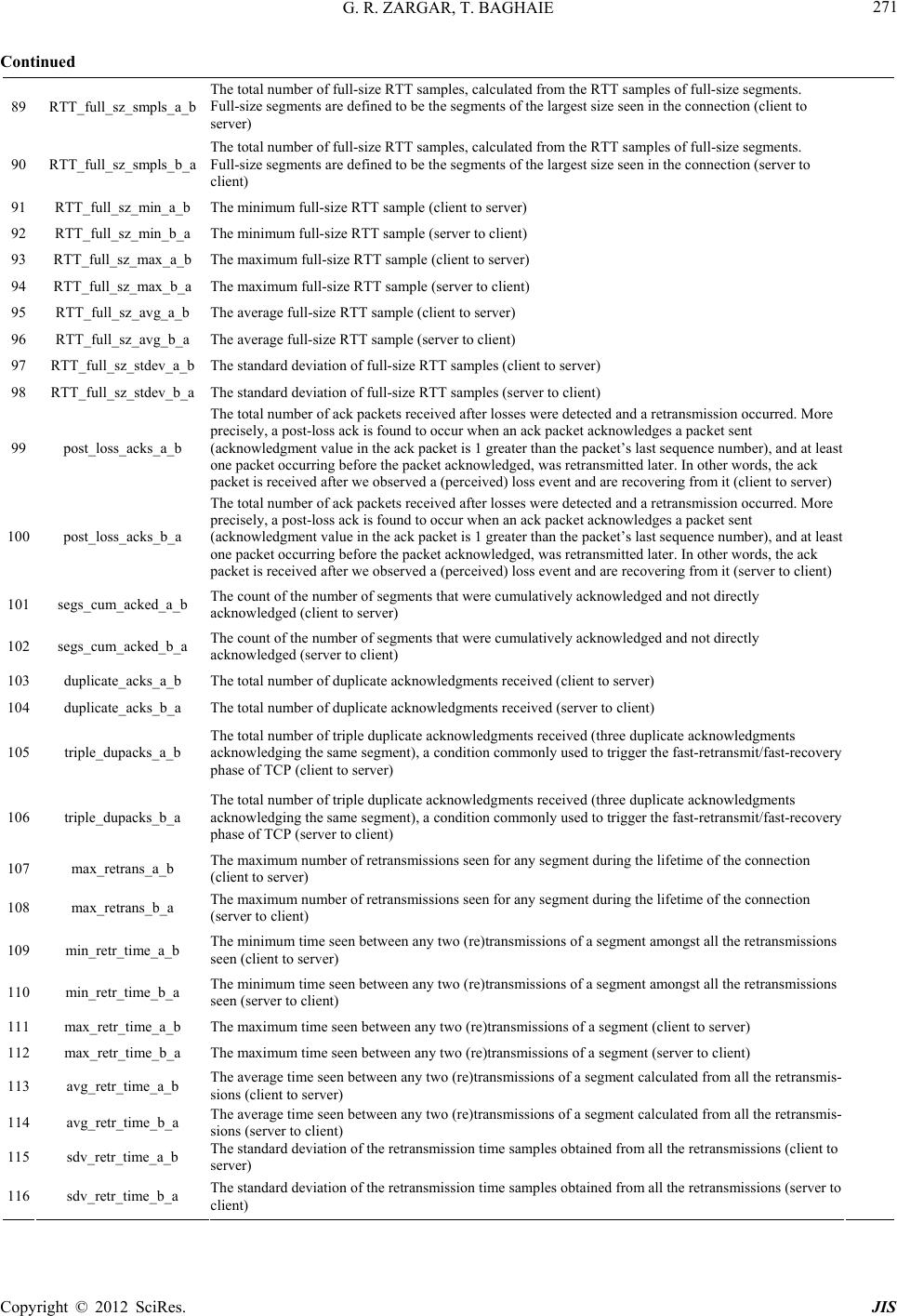 G. R. ZARGAR, T. BAGHAIE Copyright © 2012 SciRes. JIS 271 Continued RTT samples of full-size segments. t size seen in the connection (client to RTTa_b The total number of full-size RTT samples, calculated from the Full-size segments are defined to be the segments of the larges server) _full_sz_smpls_89 The total number of full-size RTT samples, calculated from the RTT samples of full-size segments. Full-size segments are defined to be the segments of the largest size seen in the connection (server to client) RTT_full_sz_smpls_b_a 90 The minimum full-size RTT sample (client to server) RTT_full_sz_min_a_b 91 The minimum full-size RTT sample (server to client) _full_sz_min_b_a RTT_full_sz_max_a_b 93 rage full-size RTT sample (client to server) RTT_full_sz_avg_a_b 95 dard deviation of full-size RTT samples (client to server) RTT_full_sz_stdev_a_b 97 r to client) re detected and a retransmission occurred. More packet acknowledges a packet sent an the packet’s last sequence number), and at least was retransmitted later. In other words, the ack event and are recovering from it (client to server) were detected and a retransmission occurred. More ck packet acknowledges a packet sent et’s last sequence number), and at least itted later. In other words, the ack e recovering from it (server to client) segs_cum_acked_a_b 101 segs_cum_acked_b_a 102 duplicate_acks_a_b 103 y triple_dupacks_a_b 105 ate acknowledgments received (three duplicate acknowledgments st-recovery ifetime of the connection ifetime of the connection max_retrans_b_a 108 min_retr_time_a_b 109 ions max_retr_time_a_b 111 is- of the retransmission time samples obtained from all the retransmissions (client to sdv_retr_time_a_b 115 of the retransmission time samples obtained from all the retransmissions (server to RTT92 The maximum full-size RTT sample (client to server) The maximum full-size RTT sample (server to client) The ave RTT_full_sz_max_b_a 94 The average full-size RTT sample (server to client) The stan RTT_full_sz_avg_b_a 96 The standard deviation of full-size RTT samples (serveRTT_full_sz_stdev_b_a 98 The total number of ack packets received after losses we precisely, a post-loss ack is found to occur when an ack (acknowledgment value in the ack packet is 1 greater th one packet occurring before the packet acknowledged, packet is received after we observed a (perceived) loss The total number of ack packets received after losses post_loss_acks_a_b 99 precisely, a post-loss ack is found to occur when an a (acknowledgment value in the ack packet is 1 greater than the pack one packet occurring before the packet acknowledged, was retransm packet is received after we observed a (perceived) loss event and ar post_loss_acks_b_a 100 The count of the number of segments that were cumulatively acknowledged and not directly acknowledged (client to server) The count of the number of segments that were cumulatively acknowledged and not directly acknowledged (server to client) The total number of duplicate acknowledgments received (client to server) The total number of duplicate acknowledgments received (server to client) The total number of triple duplicate acknowledgments received (three duplicate acknowledgments acknowledging the same segment), a condition commonly used to trigger the fast-retransmit/fast-recover duplicate_acks_b_a 104 phase of TCP (client to server) The total number of triple duplic acknowledging the same segment), a condition commonly used to trigger the fast-retransmit/fa phase of TCP (server to client) triple_dupacks_b_a 106 The maximum number of retransmissions seen for any segment during the l (client to server) The maximum number of retransmissions seen for any segment during the l max_retrans_a_b 107 (server to client) The minimum time seen between any two (re)transmissions of a segment amongst all the retransmissions seen (client to server) The minimum time seen between any two (re)transmissions of a segment amongst all the retransmiss seen (server to client) min_retr_time_b_a 110 The maximum time seen between any two (re)transmissions of a segment (client to server) The maximum time seen between any two (re)transmissions of a segment (server to client) max_retr_time_b_a 112 The average time seen between any two (re)transmissions of a segment calculated from all the retransm sions (client to server) avg_retr_time_a_b 113 The average time seen between any two (re)transmissions of a segment calculated from all the retransmis- sions (server to client) The standard deviation avg_retr_time_b_a 114 server) The standard deviation client) sdv_retr_time_b_a 116
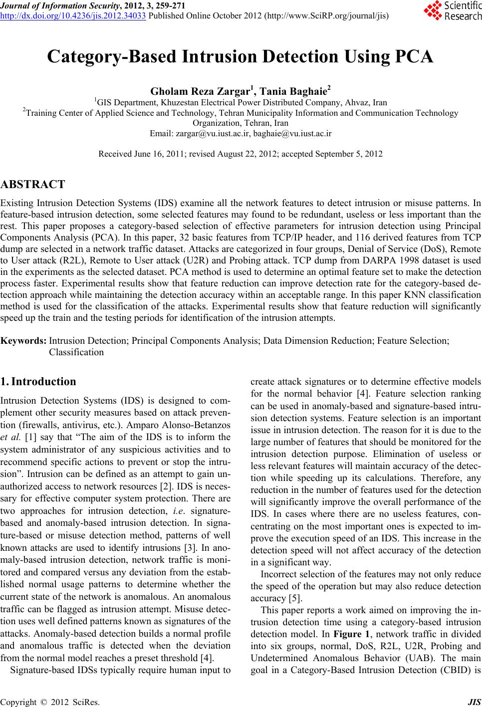
|