 International Journal of Geosciences, 2012, 3, 930-951 http://dx.doi.org/10.4236/ijg.2012.325095 Published Online October 2012 (http://www.SciRP.org/journal/ijg) Linearization of the Liouville Equation, Multiple Splits of the Chandler Frequency, Markowitz Wobbles, and Error Analysis Cheh Pan Pan Filter Technology, Saratoga, USA Email: cpan1@ix.netcom.com Received June 27, 2012; revised July 27, 2012; accepted August 29, 2012 ABSTRACT The rotation of the physical Earth is far more complex than the rotation of a biaxial or slightly triaxial rigid body can represent. The linearization of the Liouville equation via the Munk and MacDonal perturbation scheme has oversimpli- fied polar excitation physics. A more conventional linearization of the Liouville equation as the generalized equation of motion for free rotation of the physical Earth reveals: 1) The reference frame is most essential, which needs to be unique and physically located in the Earth; 2) Physical angular momentum perturbation arises from motion and mass redistribution to appear as relative angular momentum in a rotating Earth, which excites polar motion and length of day variations; 3) At polar excitation, the direction of the rotation axis in space does not change besides nutation and pre- cession around the invariant angular momentum axis, while the principal axes shift responding only to mass redistribu- tion; 4) Two inertia changes appear simultaneously at polar excitation; one is due to mass redistribution, and the other arises from the axial near-symmetry of the perturbed Earth; 5) The Earth at polar excitation becomes slightly triaxial and axially near-symmetrical even it was originally biaxial; 6) At polar excitation, the rotation of a non-rigid Earth be- comes unstable; 7) The instantaneous figure axis or mean excitation axis around which the rotation axis physically wobbles is not a principal axis; 8) In addition to amplitude excitation, the Chandler wobble possesses also multiple fre- quency-splits and is slow damping; 9) Secular polar drift is after the products of inertia and always associated with the Chandler wobble; both belong to polar motion; 10) The Earth will reach its stable rotation only after its rotation axis, major principal axis, and instantaneous figure axis or mean excitation axis are all completely aligned with each other to arrive at the minimum energy configuration of the system; 11) The observation of the multiple splits of the Chandler frequency is further examined by means of exact-bandwidth filtering and spectral analysis, which confirms the theo- retical prediction of the linearized Liouville equation. After the removal of the Gibbs phenomenon from the polar mo- tion spectra, Markowitz wobbles are also observed; 12) Error analysis of the ILS data demonstrates that the incoherent noises from the Wars in 1920-1945 are separable from polar motion and removable, so the ILS data are still reliable and useful for the study of the continuation of polar motion. Keywords: Liouville Equation; Polar Motion; Chandler Wobble; Markowitz Wobble; Error Analysis 1. Introduction It has long been known from classical mechanics that the Earth rotates like a biaxial [1,2] or slightly triaxial [3-5] rigid body. However, such a rigid model is not able to fully depict the complexity of the Earth’s rotation. The Earth is multilayered, deformable, energy-generating and dissipative. In addition to the fluidal layers of the atmos- phere, oceans and outer core, geological deformation, plate tectonics, seismicity, and volcanism observed on the Earth’s surface indicate motion and mass redistribu- tion are also to occur in the solid Earth. A renowned evi- dence for the Earth’s non-rigidity is the Chandler wobble, which is observed, as shown in Figure 1, to possess mul- tiple split-periods around fourteen months instead of a single ten-month period as predicted by the rigid model; a severe disparity. In the Eulerian equation of motion for a rigid Earth in free rotation [1,2], the Earth’s free wob- ble is due to a slight misalignment between the rotation and major principal axes; an assumed initial condition that does not physically explain, how the major principal axis of a biaxial or slightly triaxial rigid body in stable constant rotation can become misaligned with the rotation axis? The principal axis is not a vector like the rotation axis, but determined solely by matter distribution. A rigid Earth allows no motion and mass redistribution to alter its inertia for a shift of its principal axes; whereas, exter- nal torque only forces a precession of the rotation axes C opyright © 2012 SciRes. IJG  C. PAN 931 00.2 0.4 0.6 0.81 0 1 2 3 4 5 6 7 8 9 10 x 10 10 Frequenc y (c yc le/year) P ower Dens ity Sp ectra (muas **2/cpy ) P ol a r Mot ion: January 2 0, 1900 - Jan uary 20 , 20 05 x-component y-component Figure 1. The power density spectrum of polar motion of the POLE2004 series (Gross, 2005), span January 20, 1900 to January 20, 2005 at 30.4375-day intervals, where the multiple split-periods of the Chandler wobble are respec- tively, 424 days (0.861 cycle/year), 430 days (0.850 cycle/ year), 436 days (0.838 cycle/year), 442 days (0.826 cycle/ year), and 448 days (0.815 cycle/year), while the annual wobble is 365 days (1 cycle/year). The 105-year observation is not long enough to reach a full resonance cycle of the Chandler wobble. Note the presence of secular polar drift and long-period (Markowi tz) wobbles near zero-fr equency. around the invariant angular momentum axis to trace out a space cone, and not a body cone for free wobble of the rotation axis around the major principal axis. The separa- tion of the major principal axis from the rotation axis must be due to motion and mass redistribution, but which does not occur in a rigid Earth. There had been a marathon of errors in the study of polar instability [6]. Gold [7] is the first to present a con- vincing qualitative discussion on the instability of the rotation axis in an anelastic Earth. Utilizing the genera- lized Eulerian equation of motion or the Liouville equa- tion, Munk and MacDonald [8] are the first to explain the separation of the major principal axis from the rotation axis via polar excitation. Polar excitation means motion and mass redistribution are to occur in the Earth to per- turb the angular momentum, or a change in the Earth’s inertia to force the rotation axis to revolve away from the major principal axis according to the three-finger rule of the right-handed system and the law of conservation of angular momentum. This is indeed the case for a multi- layered, deformable, energy-generating, dissipative, and perpetually rotating Earth that allows motion and mass redistribution. However, as the first-time transition from a rigid rotation to a non-rigid rotation and in attempt to make the two compatible, Munk and MacDonald’s scheme [8] has oversimplified polar excitation physics, and ends up, as will see below, practically still a rigid Earth rotation but with polar excitation superimposed on independent of rotation. It hence can not predict the multi- ple splits of the Chandler frequency. The problems en- countered in the Munk and MacDonald scheme have been fragmentally investigated [9-14] and summarily discussed [15]. Geophysical problems that involve rota- tion, such as the angular momentum function of the at- mosphere, secular polar drift owing to the postglacial viscoplastic rebound, seismic excitation of the Chandler wobble, true polar wandering, and impact of a giant aste- roid or comet to the Earth, have also been re-investigated [14]. In order for a more proper depiction of the polar excitation physics, it needs a standard linearization of the Liouville equation through which the Earth’s non-rigidity is correctly represented. The present paper is a synthetic review of the linearization of the Liouville equation, as well as a systematic examination of the fundamental physics of the rotation of a non-rigid Earth that are over- simplified in the Munk and MacDonald scheme. So a thorough familiarity of the Munk and MacDonald sche- me is essential. However, non-rigidity here is still treated as what the Liouville equation allows; physical properties of the Earth are not yet added. It is an updating of fun- damental polar motion modeling to keep up with obser- vation, while the physical causes of polar excitation are not explored. Gross [16] and Gross et al. [17] identify the physical excitation of the Chandler amplitude, and Gross [18] reviewed polar motion, theory and observation, in detail. Observation of the multiple splits of the Chandler frequency is further examined here, which is consistent with the prediction of such a linearized Liouville equa- tion. However, the linearization of the Liouville equation is for free rotation of a non-rigid Earth in the absence of external torques, modeling of nutation and precession based on the Munk and MacDonald scheme [19-21] is not discussed here; related topics can be found elsewhere [13,22]. 2. Review of Rigid-Body Rotation The rotation of the Earth is conventionally cited in clas- sic mechanics as a typical case governed by the Eulerian equation of motion for a rigid body [1]; no other scien- tific models have ever lasted as long. A review of the linearization of the equation will help to see its limitation to represent the rotation of the physical Earth. For a rigid Earth, inertia tensor I is a constant and rota- tion is the only variable. The law of conservation of angular momentum requires that the rate of change of the Earth’s angular momentum in a reference frame rigidly fixed in the Earth rotating relative to an inertial frame fixed in space be equal to the external torque L exerting on the Earth; i.e., ,IL (1) Copyright © 2012 SciRes. IJG  C. PAN 932 where the over dot designates d/dt relative to the refer- ence frame fixed in the Earth. This is the well-known Eulerian equation of motion for a rigid body. Now cho- osing the Earth’s principal axes (a, b, c) as the reference frame and with constant principal inertia I = (A < B < C) and variable rotation = ( a, b, c), then, for free rota- tion of a rigid Earth at L = 0, Equation (1) expands to, –0 –0 –0. abc ac cab CB C A b BA CB A (2) Equation (2) is not linear with respect to variable so it needs to be linearized to make the equation easier to solve. Fortunately, the Earth is only slightly triaxial; i.e., C – A >> B – A and C – B >> B – A. For simplicity, let A = B; Equation (2) is then linearized as a special case for a biaxial rigid Earth in free rotation; i.e., –0 –0 ab ba CA AC , c A A (3) where is a constant. Now let CA A , or CB CAAB 0 0. ab ba . if the Earth’s slight triaxia- lity is counted [3-5], the equation further reduces to, (4) This is the equation of motion for free “Eulerian” nu- tation of a biaxial rigid Earth. Its solution gives a har- monic motion of single frequency σ, which is where the single frequency of the Chandler wobble came from. However, in the solution it needs to assume an initial condition, a slight misalignment between the rotation axis and the c-axis, to give the Chandler wobble constant amplitude. There is no physical explanation why the ro- tation axis and the c-axis of a rigid Earth in stable con- stant rotation can become separated from each other. From above brief review we see that the Eulerian equation of motion is linearized as a special case only for free rotation of a biaxial or slightly triaxial rigid Earth. If the equation is to fully represent the rotation of the phy- sical Earth, it requires: 1) The Earth has to be perfectly rigid. However, the physical Earth is a multilayered, de- formable, energy-generating, and dissipative heavenly body orbiting in space that allows motion and mass re- distribution; the Earth’s non-rigidity is totally ignored by the equation; 2) The location of the principal axes in the Earth must be known in order for the reference frame to rigidly fix to. Yet, the physical location of the Earth’s principal axes is far from certain, fixing the reference frame to them is, as Munk and MacDonald [8] have al- ready pointed out, only for mathematical simplicity. Such an idealized reference frame is inconsistent with that for observation [23]. 3) The Earth’s rotation axis and major principal axis have to be already misaligned to give con- stant wobble amplitude. However, the direction of the Earth’s rotation axis is nearly fixed in space besides nu- tation and precession, while the principal axes shift re- sponding to mass redistribution. The separation of the major principal axis from the rotation axis thus cannot occur in a rigid Earth in free rotation. 4) The Earth has to be always in stable constant rotation. On the contrary, observation shows the Earth’s rotation irregularities in- clude not only the Chandler wobble and its damping, but also secular polar drift, changes in the length of day, as well as the annual and Markowitz wobbles. All of them are not accounted for by the equation. In conclusion, the Eulerian equation of motion for a rigid body is not able to represent the complexity of the rotation of the physical Earth. It needs a generalized equation of motion, the Liouville equation, to account for the Earth’s non-rigidity, and which is what the Munk and MacDonald scheme is all after. 3. Generalized Equation of Motion: Liouville Equation Liouville equation is the generalized Eulerian equation of motion that allows motion and mass redistribution in a rotating system [8]; the physical Earth is such a rotating system, and Munk and MacDonald [8] are the first to use the Liouville equation to study the Earth’s rotation. In the equation, after the variable rotation , the inertia tensor I is also no longer a constant but subject to change, while motion and mass redistribution will induce relative an- gular momentum h. The three-finger rule of the right- handed system [2] then becomes essential. The law of conservation of angular momentum requires the rate of change of the Earth’s total angular momentum I· + h in a reference frame located in the Earth rotating relative to an inertial frame fixed in space be equal to the external torque L exerting on the Earth; i.e., Ih IhL (5) Equation (5) has three terms, h , , and × h, more than Equation (1) due to the Earth’s non-rigidity. The equation is general and the fundamental physics it represents are clear. The study of the rotation of the physical Earth is a matter of correct interpretation of the equation according to the law of conservation of angular momentum and the three-finger rule of the right-handed system. The study of the Earth’s rotation via the Liouville equa- tion needs to solve the equation. A complete solution of the equation is extremely difficult; it requires to linearize the equation for special solutions just like the Eulerian equation of motion for a rigid body in Equations (1)-(4). Copyright © 2012 SciRes. IJG  C. PAN 933 The perturbation scheme developed by Munk and Mac- Donald [8] for such a linearization laid out the founda- tion for modern Earth rotation studies [24,25]. With such a scheme, the equation is linearized to three simple first- order linear differential equations that separate the equa- torial components of the rotation from its axial compo- nent [8], just like that for the rigid Earth rotation in Equations (3) and (4). The equatorial components of the rotation can thus be mapped into a complex plan for the study of the Chandler wobble [8], while the axial com- ponent is no longer a constant as that in Equation (3) but differentiated to represent changes in the length of day. The equation explains the separation of the rotation axis from the major principal axis via polar excitation, but the axial and equatorial components of the excitation are defined not in the same dimension [8]. Such a lineariza- tion of the Liouville equation still gives the Chandler wobble a single frequency and is non-damping, while secular polar drift will not appear in the solution of the equation [23]; these are no different from what are ob- tained from Equation (4) for a rigid-body rotation, and are thus not consistent with observation [15]. What fol- lows is an exploration of these inconsistencies in the Munk and MacDonald scheme. 4. Reference Frame The reference frame is most essential, for all motions in the Earth are relative to it. For a biaxial rigid Earth, the choice is idealized: The major axis of the frame is the major principal axis, while the two equatorial axes can be aligned anywhere on the equatorial plane in the right- handed system. However, for a non-rigid Earth, as Munk and MacDonald [8] have already pointed out, it is unlikely to find a truly body-fixed frame, and frames such as Tisserand and principal axes are obvious choices for mathematical simplicity. Chao [23] examines the different theoretical frames, including Smith’s invariant frame [3], and concludes that there is an inconsistency between the frame used for observation and those for theoretical calculation. Pan [14] observes that all the conventional theoretical frames are idealized systems that are not physically located in the Earth. The frame of Mathews et al. [26] is no exception. This is because the direction of the rotation axis is not truly space-fixed ow- ing to nutation and precession; the true direction invari- ant in space is the angular momentum axis. Also, a frame cannot keep a constant rotation of its own if it is fixed to the physical Earth. Munk and MacDonald [8] align the major axis of their frame nearly parallel to the rotation axis. However, as the rotation axis traces out a body cone in the Earth, there can be an infinite number of frames with their major axis nearly parallel to the rotation axis; the frame is thus not unique. Once it is fixed to the Earth, its ap- proximation will deteriorate on the order twice the Chan- dler amplitude [12,14]. It will eventually disassociate itself from polar motion as the rotation axis revolves away to pursue after the instantaneous figure axis or mean excitation axis for polar stability. Munk and Mac- Donald [8] hence point out that their frame is not valid for polar wandering. A reference frame in the Earth should be chosen to avoid above problems; it needs to be physically located in the Earth, unique, consistent with observation, and always associated with polar motion. However, a satisfactory choice of a both theoretically and observationally practical reference frame in a rotating Earth that allows motion and mass redistribution in its different layers is most difficult. Frames may be mathe- matically transformable, but not physically. Pan [10-14] chooses a frame as that shown in Figure 2. The (a, b, c) frame is the Earth’s original principal axes prior to polar excitation, which is d iagonal; whereas, the (x, y, z) frame is the axes of the Earth’s inertia tensor that appear simul- taneously with polar excitation, which is not diagonal. The angle pair , is defined as the Earth’s axial near-symmetry, which will be further discussed below, where is the deviation angle between the c- and z-axes, and is the azimuth angle between corre- sponding equatorial axes. The frame is geocentric. Its Figure 2. The (a, b, c) frame is prior to, and (x, y, z) frame is at polar excitation. The angle pair (θ, ) is defined as the axial near-symmetry of an Earth at polar excitation. The c-axis is the original major principal axis, while z-axis is the mean excitation axis or instantaneous figure axis around which the rotation axis physically wobbles. The (x, y, z) frame is the refe rence frame. Copyright © 2012 SciRes. IJG  C. PAN 934 z-axis is the instantaneous figure axis or mean excitation axis that is aligned with the axis of reference [8] or the geographic axis [3] around which the rotation axis phy- sically wobbles. Its y-axis is along the direction of secu- lar polar drift, while x-axis is perpendicular to the y- and z-axis in the right-handed system. The Liouville equation is fully described in the frame, for it can be assumed rotating relative to an instantaneously coinciding iner- tial frame fixed in space without loss of generality [8,10, 14]. 5. Matter Perturbation and Relative Angular Momentum Physical perturbation to angular momentum arises from motion and mass redistribution in a rotating Earth. In the Munk and MacDonald scheme [8], however, first-order mathematical matter perturbation is linearly added to the principal inertia of a biaxial rigid Earth independent of rotation. Mathematically such a perturbation is legitimate but physically is unjustifiable, because it allows, as Pan [14,15] points out, the perturbed inertia to become greater than the principal inertia. If it were true, then, the Earth’s matter distribution would not be conserved, and the Earth would no longer have rotation stability. This pertains not only to internal perturbations within the Earth, but also external perturbations such as the impact of a giant meteorite or asteroid. A meteorite or asteroid becomes a part of the Earth as soon as it reaches the Earth; then, the Earth’s principal moments of inertia will again become greater than the perturbed moments of iner- tia, and the Earth’s matter distribution is still conserved. Physically, perturbing inertia appears as motion and mass redistribution about the terrestrial (x, y, z) frame rotating relative to an instantaneously coinciding inertial frame fixed in space [14]. So the differentiation operator d/dt + × applies to the whole rotating system, including h. However, in the h defined in the Munk and MacDonald scheme [8], the differentiation operator is only d/dt, which means motion is only about an inertial frame not rotating with the Earth. A single rotating system cannot have two reference frames coexisting, and motion in the system cannot bypass the rotation of the system to refer to an inertial frame that is not fixed to the system. If so, then motion in the Earth will induce no gyroscopic effect or gyricity in the Earth as is observed; this violates the three-finger rule of the right-handed system. So h has to refer to the same terrestrial (x, y, z) frame in the Earth ro- tating relative to an instantaneously coinciding inertial frame fixed in space as the whole system does. This is the fundamental physics of the rotation of a non-rigid Earth that mathematical matter perturbation is not able to represent. The motion that induces h is thus not u but u + × r, where u = (ux, uy, uz) is the motion of mass M about the (x, y, z) frame, and r = (x, y, z) is the position vector of mass M. Let be the Earth’s average rotation speed, h = (hx, hy, hz) thus becomes [10,14], , xxz yyz zz hp I hp I hp I (6) where the first term p = (px, py, pz) arises from the motion u of mass M about the (x, y, z) frame that does not in- volve rotation; i.e., d d d, y xz yxz zyx puyuzM puzuxM puxuyM 22 d d d z xz yz (7) which is identical to the relative angular momentum de- fined in the Munk and MacDonald scheme [8]. On the other hand, since the (x, y, z) frame is fixed in the Earth rotating relative to an instantaneously coinciding inertial frame fixed in space, the gyroscopic effect or gyricity from rotation to motion × r will then induce the second term in Equation (6), in which, xyM IxzM IyzM (8) are the inertia changes arising from redistribution of mass M under the gyroscopic effect or gyricity from ro- tation to motion [14,22,27]. They are named the residual moment and products of inertia by Pan [13], while Munk and MacDonald [8] define them as matter excitation. However, the mathematical matter perturbation in the Munk and MacDonald scheme [8] makes Equation (8) redundant. This forces the scheme to define the motion not to be u + ω × r but only u, bypassing the Earth’s ro- tation and directly about an inertial frame fixed in space. This is inconsistent with the whole rotating system; mo- tion in an inertial Earth is not physically feasible. The relative angular momentum in the Munk and MacDonald scheme is hence only p or Equation (7) [8], while the second term in Equation (6) or the residual inertia in Equation (8) are ignored, overlooking mass redistribution is always transported by a motion rotating with the Earth. The relative angular momentum in the scheme is thus detached from the Earth’s rotation, and is not the angular momentum perturbation arising from motion and mass redistribution in a rotating Earth as it should. This is a fundamental oversight; no motion or relative angular momentum in the physical Earth can be independent of its rotation. Pan [14] has additional discussion of the problem. The angular momentum function of the atmos- phere [15,28,30] is practically a normalized form of the relative angular momentum h in Equation (6). Fluidal Copyright © 2012 SciRes. IJG 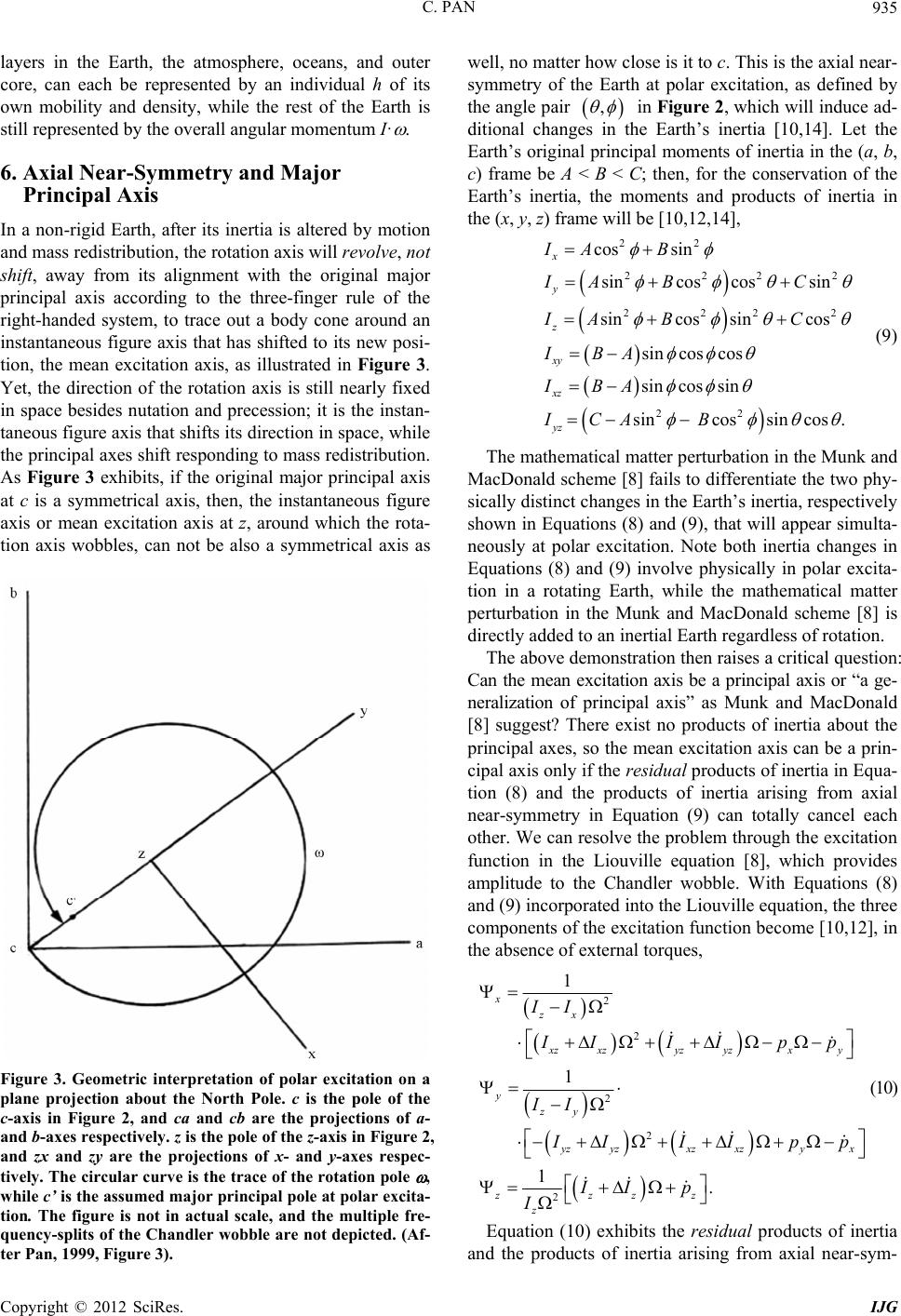 C. PAN 935 layers in the Earth, the atmosphere, oceans, and outer core, can each be represented by an individual h of its own mobility and density, while the rest of the Earth is still represented by the overall angular momentum I· . 6. Axial Near-Symmetry and Major Principal Axis In a non-rigid Earth, after its inertia is altered by motion and mass redistribution, the rotation axis will revolve, not shift, away from its alignment with the original major principal axis according to the three-finger rule of the right-handed system, to trace out a body cone around an instantaneous figure axis that has shifted to its new posi- tion, the mean excitation axis, as illustrated in Figure 3. Yet, the direction of the rotation axis is still nearly fixed in space besides nutation and precession; it is the instan- taneous figure axis that shifts its direction in space, while the principal axes shift responding to mass redistribution. As Figure 3 exhibits, if the original major principal axis at c is a symmetrical axis, then, the instantaneous figure axis or mean excitation axis at z, around which the rota- tion axis wobbles, can not be also a symmetrical axis as Figure 3. Geometric interpretation of polar excitation on a plane projection about the North Pole. c is the pole of the c-axis in Figure 2, and ca and cb are the projections of a- and b-axes respectively. z is the pole of the z-axis in Figure 2, and zx and zy are the projections of x- and y-axes respec- tively. The circular curve is the trace of the rotation pole , while c’ is the assumed major principal pole at polar excita- tion. The figure is not in actual scale, and the multiple fre- quency-splits of the Chandler wobble are not depicted. (Af- ter Pan, 1999, Figure 3). well, no matter how close is it to c. This is the axial near- symmetry of the Earth at polar excitation, as defined by the angle pair , 22 2222 2222 22 cos sin sincos cossin sincos sincos sincos cos sincos sin sin cossincos. x y z xy xz yz IA B IA BC IA BC IBA IBA ICA B in Figure 2, which will induce ad- ditional changes in the Earth’s inertia [10,14]. Let the Earth’s original principal moments of inertia in the (a, b, c) frame be A < B < C; then, for the conservation of the Earth’s inertia, the moments and products of inertia in the (x, y, z) frame will be [10,12,14], (9) The mathematical matter perturbation in the Munk and MacDonald scheme [8] fails to differentiate the two phy- sically distinct changes in the Earth’s inertia, respectively shown in Equations (8) and (9), that will appear simulta- neously at polar excitation. Note both inertia changes in Equations (8) and (9) involve physically in polar excita- tion in a rotating Earth, while the mathematical matter perturbation in the Munk and MacDonald scheme [8] is directly added to an inertial Earth regardless of rotation. The above demonstration then raises a critical question: Can the mean excitation axis be a principal axis or “a ge- neralization of principal axis” as Munk and MacDonald [8] suggest? There exist no products of inertia about the principal axes, so the mean excitation axis can be a prin- cipal axis only if the residual products of inertia in Equa- tion (8) and the products of inertia arising from axial near-symmetry in Equation (9) can totally cancel each other. We can resolve the problem through the excitation function in the Liouville equation [8], which provides amplitude to the Chandler wobble. With Equations (8) and (9) incorporated into the Liouville equation, the three components of the excitation function become [10,12], in the absence of external torques, 2 2 2 2 2 1 1 1. x zx xz xzyz yzxy y zy zyzxzxzy x zzzz z II IIII pp II IIIpp II p I (10) Equation (10) exhibits the residual products of inertia and the products of inertia arising from axial near-sym- Copyright © 2012 SciRes. IJG 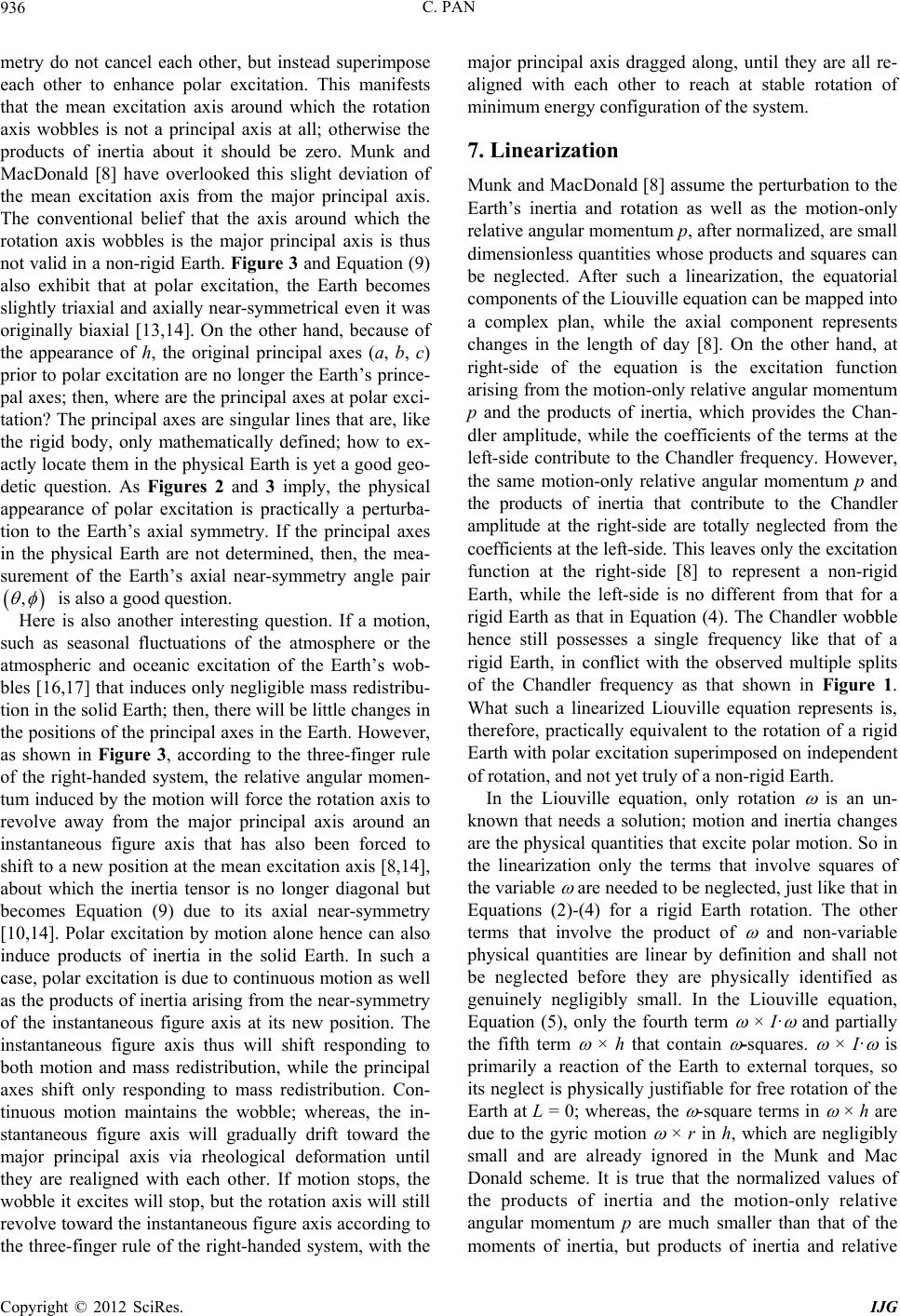 C. PAN 936 metry do not cancel each other, but instead superimpose each other to enhance polar excitation. This manifests that the mean excitation axis around which the rotation axis wobbles is not a principal axis at all; otherwise the products of inertia about it should be zero. Munk and MacDonald [8] have overlooked this slight deviation of the mean excitation axis from the major principal axis. The conventional belief that the axis around which the rotation axis wobbles is the major principal axis is thus not valid in a non-rigid Earth. Figure 3 and Equation (9) also exhibit that at polar excitation, the Earth becomes slightly triaxial and axially near-symmetrical even it was originally biaxial [13,14]. On the other hand, because of the appearance of h, the original principal axes (a, b, c) prior to polar excitation are no longer the Earth’s prince- pal axes; then, where are the principal axes at polar exci- tation? The principal axes are singular lines that are, like the rigid body, only mathematically defined; how to ex- actly locate them in the physical Earth is yet a good geo- detic question. As Figures 2 and 3 imply, the physical appearance of polar excitation is practically a perturba- tion to the Earth’s axial symmetry. If the principal axes in the physical Earth are not determined, then, the mea- surement of the Earth’s axial near-symmetry angle pair , is also a good question. Here is also another interesting question. If a motion, such as seasonal fluctuations of the atmosphere or the atmospheric and oceanic excitation of the Earth’s wob- bles [16,17] that induces only negligible mass redistribu- tion in the solid Earth; then, there will be little changes in the positions of the principal axes in the Earth. However, as shown in Figure 3, according to the three-finger rule of the right-handed system, the relative angular momen- tum induced by the motion will force the rotation axis to revolve away from the major principal axis around an instantaneous figure axis that has also been forced to shift to a new position at the mean excitation axis [8,14], about which the inertia tensor is no longer diagonal but becomes Equation (9) due to its axial near-symmetry [10,14]. Polar excitation by motion alone hence can also induce products of inertia in the solid Earth. In such a case, polar excitation is due to continuous motion as well as the products of inertia arising from the near-symmetry of the instantaneous figure axis at its new position. The instantaneous figure axis thus will shift responding to both motion and mass redistribution, while the principal axes shift only responding to mass redistribution. Con- tinuous motion maintains the wobble; whereas, the in- stantaneous figure axis will gradually drift toward the major principal axis via rheological deformation until they are realigned with each other. If motion stops, the wobble it excites will stop, but the rotation axis will still revolve toward the instantaneous figure axis according to the three-finger rule of the right-handed system, with the major principal axis dragged along, until they are all re- aligned with each other to reach at stable rotation of minimum energy configuration of the system. 7. Linearization Munk and MacDonald [8] assume the perturbation to the Earth’s inertia and rotation as well as the motion-only relative angular momentum p, after normalized, are small dimensionless quantities whose products and squares can be neglected. After such a linearization, the equatorial components of the Liouville equation can be mapped into a complex plan, while the axial component represents changes in the length of day [8]. On the other hand, at right-side of the equation is the excitation function arising from the motion-only relative angular momentum p and the products of inertia, which provides the Chan- dler amplitude, while the coefficients of the terms at the left-side contribute to the Chandler frequency. However, the same motion-only relative angular momentum p and the products of inertia that contribute to the Chandler amplitude at the right-side are totally neglected from the coefficients at the left-side. This leaves only the excitation function at the right-side [8] to represent a non-rigid Earth, while the left-side is no different from that for a rigid Earth as that in Equation (4). The Chandler wobble hence still possesses a single frequency like that of a rigid Earth, in conflict with the observed multiple splits of the Chandler frequency as that shown in Figure 1. What such a linearized Liouville equation represents is, therefore, practically equivalent to the rotation of a rigid Earth with polar excitation superimposed on independent of rotation, and not yet truly of a non-rigid Earth. In the Liouville equation, only rotation is an un- known that needs a solution; motion and inertia changes are the physical quantities that excite polar motion. So in the linearization only the terms that involve squares of the variable are needed to be neglected, just like that in Equations (2)-(4) for a rigid Earth rotation. The other terms that involve the product of and non-variable physical quantities are linear by definition and shall not be neglected before they are physically identified as genuinely negligibly small. In the Liouville equation, Equation (5), only the fourth term × I· and partially the fifth term × h that contain -squares. × I· is primarily a reaction of the Earth to external torques, so its neglect is physically justifiable for free rotation of the Earth at L = 0; whereas, the -square terms in × h are due to the gyric motion × r in h, which are negligibly small and are already ignored in the Munk and Mac Donald scheme. It is true that the normalized values of the products of inertia and the motion-only relative angular momentum p are much smaller than that of the moments of inertia, but products of inertia and relative Copyright © 2012 SciRes. IJG  C. PAN 937 angular momentum are neither in the same physical dimension nor on the same order of magnitude, and their normalized values are not necessarily negligibly small or physically insignificant in comparison to the normalized differences of the axial and equatorial moments of inertia; the latter comprises the fundamental Chandler frequency constituents. On the other hand, if motion and mass redistribution can excite the Chandler amplitude, there is no reason to assume that they are too small to affect the Chandler frequency. It is hence inappropriate to neglect them before they are physically identified indeed too small to contribute to the Chandler frequency. Take into account of above considerations and let the only mathe- matical perturbation be = (mx, my, 1 + mz), where (mx, my, mz) are dimensionless small quantities [8], the lineari- zation of the Liouville equation in the absence of external torques becomes [10,12], 2 () 2 xyxxyxy z xy xx yzxz y xz zz xx xyxy z y y x yy xy y xx yy yzxzyz x zz yy yzxz yyz xz xx zz xz yz II I mmm II IIh Imm II IIh mm II IIIh mm II IIh I Imm II II y y y xx y z Ih m I II mm I m I , z yz yz z zz hI mm m II (11) where zx y x I I and zy y x II I ,, are not inde- pendent components but the constituents of the funda- mental Chandler frequency arising from matter distribu- tion in a slightly triaxial and axially near-symmetrical Earth [12], and yz is the excitation function in Equation (10). The coefficients of left-side terms in Equation (11) provide frequencies to the Chandler wob- ble, thus not only moments of inertia but also products of inertia and motion will contribute to the Chandler fre- quency [12]. Equation (11) is three dimensional, and its x- and y-components can no longer be mapped into a complex plan mathematically as that in the Munk and MacDonald scheme [8]. The solution of Equation (11) [10,12] gives a slow damping Chandler wobble of multiple frequency-splits as well as secular polar drift, consistent with the observation that the Chandler wobble hardly changes except exhibiting a “beat” phenomenon of resonant coupled oscillations [8,12,15,31,32]. This confirms that single frequency is not the intrinsic property of the Chandler wobble, but is only for the free rotation of a biaxial or slightly triaxial rigid Earth under an assumed initial condition of a slight misalignment be- tween the rotation and major principal axes. The ob- servation of apparent single Chandler frequency is be- cause the length of data analyzed is shorter than the resonance cycle and in a time span within the modulation envelope of the oscillations [15]. The solution of Equation (11) [10,12] is very compli- cated. In the solution [12], the wobble frequency consists of a natural frequency plus or minus three small feedback frequency series that are equivalent to adding of small springs and dashpots in series with the main oscillator. Yet, the natural frequency can further be separated into a fundamental frequency attributing to the Earth’s slight triaxiality just like that of a rigid Earth, and also three small feedback frequency series that are equivalent to adding of small springs and dashpots in parallel with the main oscillator. Such a feedback mechanism causes the multiple splits of the Chandler frequency. The small feedback frequency series are due respectively to instan- taneous inertia, relative angular momentum, and inertia variation arising from the same motion and mass redis- tribution that excite the Chandler amplitude [16-18]. However, physical details of the frequency excitation are not yet identified; the Liouville equation and its solution can be further simplified if the orders of magnitude of some of the terms are physically identified to be negligi- bly small. 8. Rotation Instability The solution of Equation (11) [10,12] gives an exponen- tially damping Chandler wobble together with an ex- ponentially increasing secular polar drift, suggesting the Earth’s rotation is unstable. Secular polar drift represents the Earth’s attempt to eliminate its products of inertia, so it is always associated with the Chandler wobble that is also involved with the products of inertia [14,22]; they together constitute polar motion for the Earth to seek rotation stability. The damping relaxation time for a Chandler wobble of multiple frequency-splits is on the order of 104 to 106 years [12], and available observation [15] indicates the Chandler wobble has yet to reach a complete multiple-resonance cycle. In a multilayered, deformable, energy-generating and dissipative Earth, once the rotation, major principal, and instantaneous figure axes are separated from each other, they will no longer be able to revert back to their original position of alignment in the Earth again, while rheological equatorial bulge will migrate with secular polar drift accordingly [8]; so it is an unstable rotation. In an Earth in unstable Copyright © 2012 SciRes. IJG  C. PAN 938 rotation, secular internal torques [10,13,22], particularly those due to the gyroscopic effect or gyricity from rotation to motion [13,22,27], dominate secular global geodynamics and also cause free nutation. The Earth will reach a stable rotation via self-deformation and quadru- polar adjustment according to the law of conservation of angular momentum and the three-finger rule of the right-handed system, until its rotation, major principal, and instantaneous figure axes are all completely realig- ned with each other to arrive at the minimum energy configuration of the system [14]. Then, (mx, my, mz) = 0, , and (x, y, z) = (a, b, c). ,0 9. Chandler and Markowitz Wobbles, Secular Polar Drift Assuming the Chandler wobble to be a complex time series, Okubo [33] tests the variability of the Chandler amplitude, and concludes that it is an artifact depending on the analysis methods. Here we further examine this particular problem via direct analysis of observation, to see whether the multiple splits of the Chandler frequency are artifacts. The data used for this analysis is the 105- year POLE2004 series [15,34], which is, as error- analysis below will show, reliable and useful for the study of the continuation of polar motion. Complex Liou- ville equation [8] predicts only a non-damping single- frequency Chandler wobble with no secular polar drift, as if the Earth were rigid after an amplitude excitation. It is therefore not appropriate to map real observations into a complex plan for the analysis of the frequency excitation it does not cover; our analysis reflects Equation (11). The analysis tool is a simplest radix-2 FFT; no further assumptions or parameters are added to generate artifacts. All artifacts in an FFT are due to the finite truncation of input, and among them only the Gibbs phenomenon smears the whole spectrum; the others are uncom- pensated spectral leakages at local frequencies that will neither contaminate the signals nor transfer to the time domain to induce amplitude modulation. So after the Gibbs phenomenon is removed, no other artifacts will smear the spectra or induce amplitude modulation, while digital filtering is exact, not approximation like conven- tional filters. We start from Figure 1, the power density spectrum of the POLE2004 series from 0.0 to 1.1 cycle/year, includ- ing secular polar drift, Markowitz, Chandler, and annual wobbles as well as background noises. There is no Gibbs phenomenon in a power density spectrum, so the baseline tilting method [15,35] that removes the Gibbs pheno- menon but will introduce a near-DC component into the spectrum, is not applied. What in Figure 1 are thus either input signals/noises or uncompensated leakages due to finite truncation of the input. For the study of the Chan- dler wobble, we remove the annual wobble from polar motion, it then gives a waveform as that in Figure 4 and a power density spectrum in Figure 5. Pan [15] observes that the bandwidth of the Chandler wobble is a constant 0.79 - 0.875 cycle/year regardless of data length, data quality, time span, and time sampling rate; whereas, that of the annual wobble varies from 0.99 - 1.01 cycle/year for the 105-year (1900-2005) POLE- 2004 series at 30.4375-day intervals to a broader 0.975 - 1.025 cycle/year for the more modern 42-year (1962- 2005) COMB2004 series at daily intervals. A broad band- width consists of more than a single discrete frequency even it has only a single peak [15]. The Chandler spec- trum splits within its bandwidth with the increase of time span regardless of time sampling rate, but the annual wobble only shifts its frequency content. This exhibits that the annual wobble varies timely in response to seasonal fluctuations of the atmosphere; whereas, splits of Chandler frequency reflect the amplitude modulation cycles within the time span [15]. The Gibbs phenomenon is already removed, and spectral leakages will not contaminate the wobble frequencies, so the splits within the constant bandwidth all belong to the Chandler com- ponents that will induce amplitude modulation in the time span. To further look into it, we isolate the Chandler bandwidth; its power density spectrum is shown in Figure 6, and waveform in Figure 7 (also [15]). A com- parison of Figures 4 and 7, we can see that their dif- ference is only that Figure 4 still contains all the remain- ders of polar motion, secular polar drift, the Markowitz wobbles, and background noises except the annual wobble, while Figure 7 consists of only what is within the Chandler bandwidth. Figures 4 and 7 reflect each other; both exhibit the resonant oscillations or amplitude modulation cycles that a single-frequency wobble cannot have. However, there is a general belief that if the Chan- dler frequency is to split, it is a single split [31,32,36,37]. So one may still suspect the side-splits of the Chandler frequency are artifacts. To test this, we remove the side- splits from the Chandler frequency. This is equivalent to spectral leakages are totally compensated as if the input length were infinite, which hence will not affect the signals. Figure 8 is the power density spectrum of the main-split and Figure 9 is its waveform, which displays a typical single coupled oscillation obviously different from the multiple amplitude modulations as that in Fig- ures 4 and 7. A comparison of Figures 7 and 9, we can easily conclude that the side-splits cannot be artifacts but belong to the Chandler components, for artifacts or spectral leakages are not able to add to the main-split to induce the multiple amplitude modulations beyond a single coupled oscillationas that shown in Figure 7. For further confirmation, it is also of interest to see how the side-splits alone wil behave. Figure 10 is the l Copyright © 2012 SciRes. IJG  C. PAN Copyright © 2012 SciRes. IJG 939 1900 1910192019301940 195019601970 19801990 2000 -4 -2 0 2 4 6x 10 5 Time (year) X-Com pon en t (mu as) Polar motion with annual wobble removed: January 20, 1900 - J anuary 20, 2005 1900 1910192019301940 195019601970 19801990 2000 -4 -2 0 2 4 6x 10 5 Time (year) Y-Com p one nt (mu as) Figure 4. Polar motion of the POLE2004 series (Gross, 2005) with annual wobble removed, span January 20, 1900 to January 20, 2005 at 30.4375-day intervals. 00.20.4 0.6 0.8 1 0 1 2 3 4 5 6 7 8 9 10 x 10 10 Frequency ( cycle/year) Power Density Spe ctra (mua s**2/cpy) Polar motion wi th annual wobble r emoved: January 20, 1900 - Januar y 20, 2005 x-component y- component Figure 5. The power density spectrum of polar motion of the POLE2004 series (Gross, 2005) with annual wobble removed, span January 20, 1900 to January 20, 2005 at 30.4375-day intervals.  C. PAN 940 00.2 0.4 0.60.8 1 0 1 2 3 4 5 6 7 8 9 10 x 10 10 Frequency ( c yc le/year) Power Density Spectra (muas ** 2/cpy ) The C handler wobble only : January 20, 1900 - January 20, 200 5 x-com ponent y-component Figure 6. The power density spectrum of the Chandler wobble from the POLE2004 series (Gross, 2005), span January 20, 1900 to January 20, 2005 at 30.4375-day intervals. 1900 19101920 19301940195019601970 1980 1990 2000 -4 -2 0 2 4 6x 10 5 Time (year) X-Component (mu as) The C handler wobble only: J anuary 20, 1900 - January 20, 2005 1900 1910192019301940 1950 19601970 198019902000 -4 -2 0 2 4 6x 10 5 Time (year) Y-Component (mu as) Figure 7. The Chandler wobble from the POLE2004 series (Gross, 2005), span January 20, 1900 to January 20, 2005 at 30.4375-day intervals. Copyright © 2012 SciRes. IJG  C. PAN 941 00.20.4 0.60.8 1 0 1 2 3 4 5 6 7 8 9 10 x 10 10 Frequenc y ( cycle/yea r) Power Density S pectra (muas**2/c py) The C handler wobble mai n-split only: January 20, 1900 - J anuary 20 , 2005 x-component y- component Figure 8. The power density spectrum of the main-split of the Chandler wobble from the POLE2004 series (Gross, 2005), span January 20, 1900 to January 20, 2005 at 30.4375-day intervals. 1900 1910 1920 19301940 1950 1960 19701980 19902000 -4 -2 0 2 4 6x 10 5 Time (y ear) X-Com ponent (mu as) The C handler wobble main-split only: Januar y 20, 1900 - January 20, 2005 1900 1910 1920 19301940 1950 1960 19701980 19902000 -4 -2 0 2 4 6x 10 5 Time (y ear) Y-Compon ent (mu as) Figure 9. The waveform of the main-split of the Chandler wobble from the POLE2004 series (Gross, 2005), span January 20, 1900 to January 20, 2005 at 30.4375-day intervals. Copyright © 2012 SciRes. IJG  C. PAN Copyright © 2012 SciRes. IJG 942 0.6 0.650.70.75 0.8 0.850.9 0.95 11.051.1 0 0.5 1 1.5 2 2.5 3 3.5 4x 10 10 Frequency ( cyc le/year) Power Density Spectra (muas**2/cpy) The C handler side-splits: January 20, 1900 - J anuary 20, 2005 x-component y- component Figure 10. The power density spectrum of the side-splits of the Chandler wobble from the POLE2004 series (Gross, 2005), span January 20, 1900 to January 20, 2005 at 30.4375-day intervals. power density spectrum of the side-splits and Figure 11 is its waveform, which further exhibit that the side-splits are not leakages but components of the resonant oscilla- tions of the Chandler wobble that are missed in Figures 8 and 9. Note in Figure 10 there are two non-zero uncom- pensated leakage peaks within the original bandwidth of the main-split, but which will not contaminate the side- splits or induce amplitude modulations in the time domain. In Figure 11, the magnitude of the amplitude modulation is slowly decreasing, which may reflect the imbalances of the splits at each side of the removed main-split. We now remove both the Chandler and annual wobbles wholly to see how the remainders of polar motion will behave; Figure 12 is the power density spectrum and Figure 13 is the waveform. The remainders in Figure 12 are secular polar drift, the Markowitz wobbles, back- ground noises, as well as uncompensated leakages. How- ever, as what is shown in Figure 13, none of the re- mainders will generate resonant oscillations or amplitude modulations. This further exhibits that artifacts or uncompensated spectral leakages have nothing to do with the multiple splits of the Chandler frequency. In Figure 1 or 4 we can also find that near the zero- frequency of the power density spectrum, there exist three conspicuous and one minor spectral peaks in the x-component. The y-component is dominated by secular polar drift, but there are yet two peaks that can be identified corresponding to those in the x-component. Figure 14 plots the enlarged part of the spectrum from 0.0 to 0.3 cycle/year, and Table 1 lists the measurements of those low-frequency spectral peaks. Because of the do- mination of secular polar drift in this near-DC frequency range, only two peaks, respectively at 0.029 cycle/year (34.48 years) and at 0.047 cycle/year (21.28 years), can be commonly identified from both the x- and y- com- ponents, which are close to the Markowitz wobble. Gross [18] reports the Markowitz wobble has a period of 24 years and an amplitude of 30 mas. The wobbles in this frequency range are within or close to the bandwidth of secular polar drift; their measurements are therefore corrupted by it and are also heavily dependent on spectral resolution. The corruption of the wobbles by secular polar drift is another reason that to map polar motion into a complex plan may be misleading. However, what listed in Table 1 are yet apparent and cannot be taken too seriously. Longer observation is needed for more detailed study of these long-period wobbles. It is not yet certain whether Equation (11) will predict such long-period wobbles. If it does not, then they are not free wobbles. Finally, we can also make a glance at secular polar drift. Based on Figure 14, we pick 0.000 - 0.012 cycle/ year as its bandwidth. Then, its power density spectrum is shown in Figure 15, and waveform is plotted together with the original polar motion observation in Figure 16. 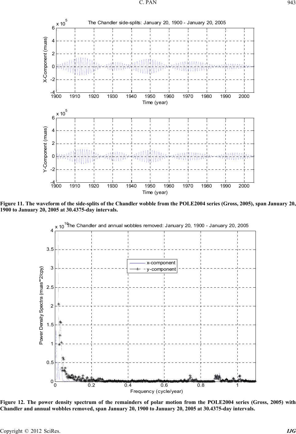 C. PAN 943 1900 19101920 19301940 195019601970 1980 1990 2000 -4 -2 0 2 4 6x 10 5 Time (y ear) X-Compon ent (mu as) The Chandler side-splits: January 20, 1900 - January 20, 2005 1900 19101920 19301940 195019601970 1980 1990 2000 -4 -2 0 2 4 6x 10 5 Time (y ear) Y-Compon ent (mu as) Figure 11. The waveform of the side-splits of the Chandler wobble from the POLE2004 series (Gross, 2005), span January 20, 1900 to January 20, 2005 at 30.4375-day intervals. 00.20.4 0.6 0.8 1 0 0.5 1 1.5 2 2.5 3 3.5 4x 10 10 Frequency ( cycle/year) Power Density Spectra (muas**2/c py) The Chandler and annual wobbles removed: J anuary 20, 1900 - J anuar y 20, 2005 x-com p onent y- component Figure 12. The power density spectrum of the remainders of polar motion from the POLE2004 series (Gross, 2005) with Chandler and annual wobbles removed, span January 20, 1900 to January 20, 2005 at 30.4375-day intervals. Copyright © 2012 SciRes. IJG 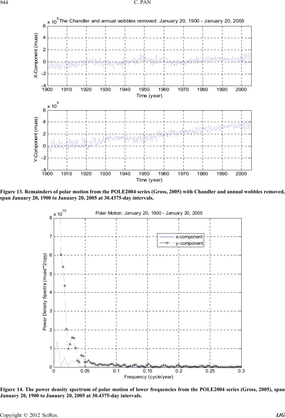 C. PAN 944 1900 191019201930 19401950 1960 1970 198019902000 -4 -2 0 2 4 6x 10 5 Time (ye a r) X-Com pon en t (mu as) The Chandler and annual wobbles removed: J anuar y 20, 1900 - J anuar y 20, 2005 1900 191019201930 19401950 1960 1970 198019902000 -4 -2 0 2 4 6x 10 5 Time (ye a r) Y-Com ponent (mu as) Figure 13. Remainders of polar motion from the POLE2004 series (Gross, 2005) with Chandler and annual wobbles removed, span January 20, 1900 to January 20, 2005 at 30.4375-day intervals. 00.05 0.10.15 0.2 0.25 0.3 0 1 2 3 4 5 6 7 8x 10 10 Frequency ( c yc le/year) Power Density Spectra (muas**2/cpy) Polar Motion: January 20, 1900 - J anuary 20, 2005 x-component y- component Figure 14. The power density spectrum of polar motion of lower frequencies from the POLE2004 series (Gross, 2005), span January 20, 1900 to January 20, 2005 at 30.4375-day intervals. Copyright © 2012 SciRes. IJG  C. PAN 945 Table 1. The long-period (markowitz) wobbles. Frequency (cycle/year) 0.006 0.018 0.029 0.047 Period (year) 166.67 55.56 34.48 21.28 x-amplitude (μas) 4.1 × 10⁵ 2.5 × 10⁵ 2.0 × 10⁵ 0.7 × 10⁵ y-amplitude (μas) 4.4 × 10⁵ 2.7 × 10⁵ 00.050.1 0.15 0.2 0.25 0.3 0.35 0.4 0 1 2 3 4 5 6 7 8 9x 10 11 Frequency ( c ycle/year) Power Density Spectra (muas**2/cpy) Sec ular Polar Dri ft: J anuary 20, 1900 - J anuary 20, 2005 x-component y -component Figure 15. The power density spectrum of secular polar drift from the POLE2004 series (Gross, 2005), span January 20, 1900 to January 20, 2005 at 30.4375-day intervals. 1900 1910 1920 1930 1940 1950 1960 1970 19801990 2000 -4 -2 0 2 4 6x 10 5 Time (y ear) X-Compon ent (muas) Polar Motion and Secular Polar Dr ift: J anuar y 20, 1900 - J anuary 20, 2005 1900 1910 1920 1930 1940 1950 1960 1970 19801990 2000 -4 -2 0 2 4 6x 10 5 Time (y ear) Y-Compon ent (muas) Polar motion Secular polar drift Figure 16. Secular polar drift and polar motion from the POLE2004 series (Gross, 2005), span January 20, 1900 to January 0, 2005 at 30.4375-day intervals. 2 Copyright © 2012 SciRes. IJG 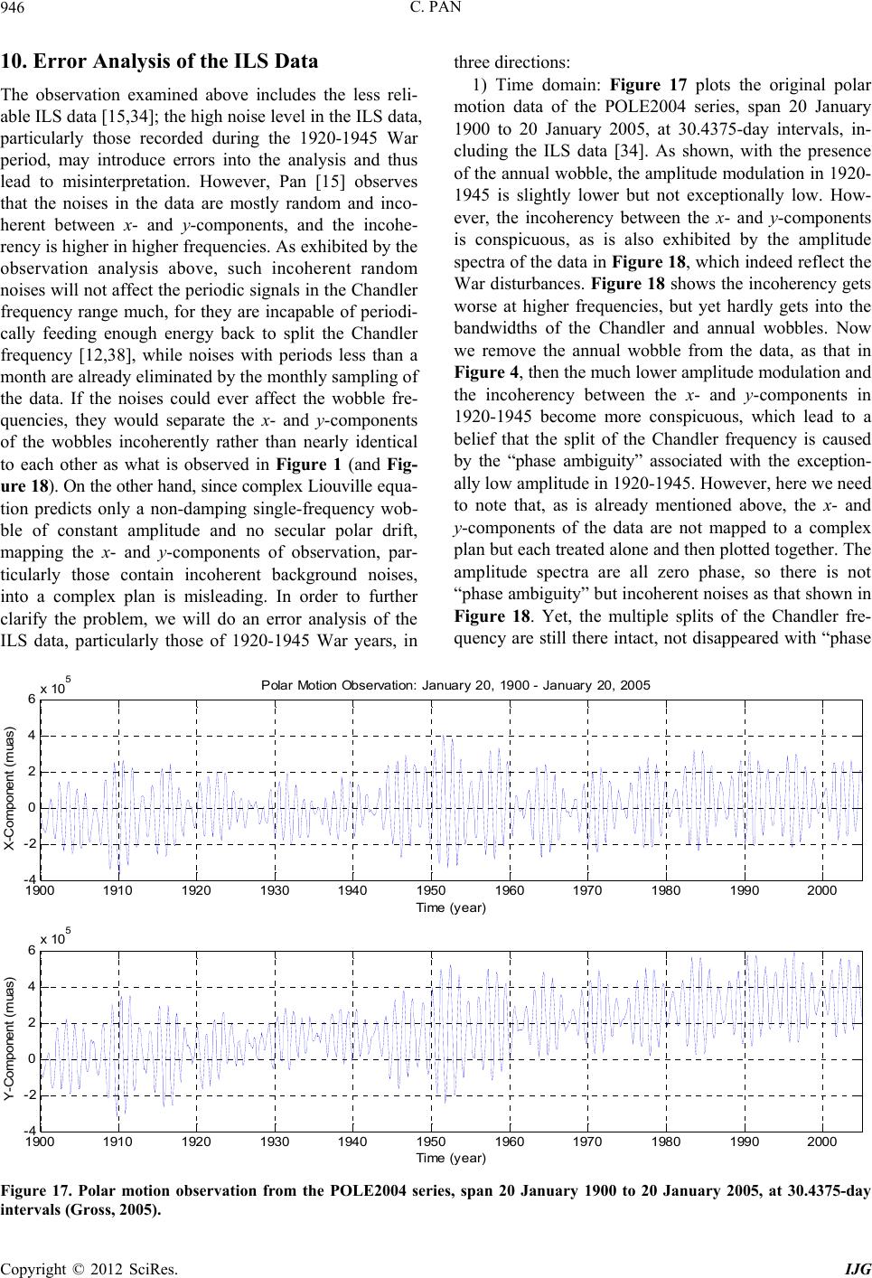 C. PAN Copyright © 2012 SciRes. IJG 946 10. Error Analysis of the ILS Data The observation examined above includes the less reli- able ILS data [15,34]; the high noise level in the ILS data, particularly those recorded during the 1920-1945 War period, may introduce errors into the analysis and thus lead to misinterpretation. However, Pan [15] observes that the noises in the data are mostly random and inco- herent between x- and y-components, and the incohe- rency is higher in higher frequencies. As exhibited by the observation analysis above, such incoherent random noises will not affect the periodic signals in the Chandler frequency range much, for they are incapable of periodi- cally feeding enough energy back to split the Chandler frequency [12,38], while noises with periods less than a month are already eliminated by the monthly sampling of the data. If the noises could ever affect the wobble fre- quencies, they would separate the x- and y-components of the wobbles incoherently rather than nearly identical to each other as what is observed in Figure 1 (and Fig- ure 18). On the other hand, since complex Liouville equa- tion predicts only a non-damping single-frequency wob- ble of constant amplitude and no secular polar drift, mapping the x- and y-components of observation, par- ticularly those contain incoherent background noises, into a complex plan is misleading. In order to further clarify the problem, we will do an error analysis of the ILS data, particularly those of 1920-1945 War years, in three directions: 1) Time domain: Figure 17 plots the original polar motion data of the POLE2004 series, span 20 January 1900 to 20 January 2005, at 30.4375-day intervals, in- cluding the ILS data [34]. As shown, with the presence of the annual wobble, the amplitude modulation in 1920- 1945 is slightly lower but not exceptionally low. How- ever, the incoherency between the x- and y-components is conspicuous, as is also exhibited by the amplitude spectra of the data in Figure 18, which indeed reflect the War disturbances. Figure 18 shows the incoherency gets worse at higher frequencies, but yet hardly gets into the bandwidths of the Chandler and annual wobbles. Now we remove the annual wobble from the data, as that in Figure 4, then the much lower amplitude modulation and the incoherency between the x- and y-components in 1920-1945 become more conspicuous, which lead to a belief that the split of the Chandler frequency is caused by the “phase ambiguity” associated with the exception- ally low amplitude in 1920-1945. However, here we need to note that, as is already mentioned above, the x- and y-components of the data are not mapped to a complex plan but each treated alone and then plotted together. The amplitude spectra are all zero phase, so there is not “phase ambiguity” but incoherent noises as that shown in Figure 18. Yet, the multiple splits of the Chandler fre- quency are still there intact, not disappeared with “phase 1900 1910 19201930 194019501960 1970 1980 1990 6x 10 5 2000 -4 -2 0 2 4 Time (ye a r) X-Com pon ent (mu as) Polar Motion Observation: January 20, 1900 - January 20, 2005 1900 1910 19201930 194019501960 1970 1980 1990 6x 10 5 2000 -4 -2 0 2 4 Time (ye a r) Y-Com pon ent (mu as) Figure 17. Polar motion observation from the POLE2004 series, span 20 January 1900 to 20 January 2005, at 30.4375-day intervals (Gross, 2005). 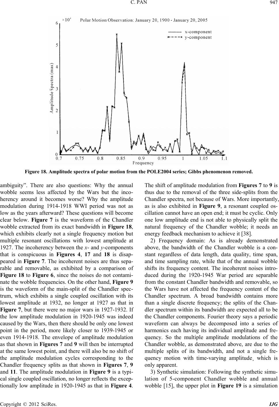 C. PAN 947 Figure 18. Amplitude spectra of polar motion from the POLE2004 series; Gibbs phenomenon removed. ambiguity”. There are also questions: Why the annual wobble seems less affected by the Wars but the inco- herency around it becomes worse? Why the amplitude modulation during 1914-1918 WWI period was not as low as the years afterward? These questions will become clear below. Figure 7 is the waveform of the Chandler wobble extracted from its exact bandwidth in Figure 18, which exhibits clearly not a single frequency motion but multiple resonant oscillations with lowest amplitude at 1927. The incoherency between the x- and y-components that is conspicuous in Figures 4, 17 and 18 is disap- peared in Figure 7. The incoherent noises are thus sepa- rable and removable, as exhibited by a comparison of Figure 18 to Figure 6, since the noises do not contami- nate the wobble frequencies. On the other hand, Figure 9 is the waveform of the main-split of the Chandler spec- trum, which exhibits a single coupled oscillation with its lowest amplitude at 1932, no longer at 1927 as that in Figure 7, but there were no major wars in 1927-1932. If the low amplitude modulation in 1920-1945 was indeed caused by the Wars, then there should be only one lowest point in the period, more likely closer to 1939-1945 or even 1914-1918. The envelope of amplitude modulation as that shown in Figures 7 and 9 will then be interrupted at the same lowest point, and there will also be no shift of the amplitude modulation cycles corresponding to the Chandler frequency splits as that shown in Figures 7, 9 and 11. The amplitude modulation in Figure 9 is a typi- cal single coupled oscillation, no longer reflects the excep- tionally low amplitude in 1920-1945 as that in Figure 4. The shift of amplitude modulation from Figures 7 to 9 is thus due to the removal of the three side-splits from the Chandler spectra, not because of Wars. More importantly, as is also exhibited in Figure 9, a resonant coupled os- cillation cannot have an open end; it must be cyclic. Only one low amplitude end is not able to physically split the natural frequency of the Chandler wobble; it needs an energy feedback mechanism to achieve it [38]. 2) Frequency domain: As is already demonstrated above, the bandwidth of the Chandler wobble is a con- stant regardless of data length, data quality, time span, and time sampling rate, while that of the annual wobble shifts its frequency content. The incoherent noises intro- duced during the 1920-1945 War period are separable from the constant Chandler bandwidth and removable, so the Wars have not affected the frequency content of the Chandler spectrum. A broad bandwidth contains more than a single discrete frequency; the splits of the Chan- dler spectrum within its bandwidth are expected all to be the Chandler components. Fourier theory says a periodic waveform can always be decomposed into a series of harmonics each having its individual amplitude and fre- quency. So the multiple amplitude modulations of the Chandler wobble, as demonstrated above, are due to the multiple splits of its bandwidth, and not a single fre- quency motion with time-varying amplitude¸ which is only apparent. 3) Synthetic simulation: Following the synthetic simu- lation of 5-component Chandler wobble and annual wobble [15], the upper plot in Figure 19 is a simulation Copyright © 2012 SciRes. IJG  C. PAN 948 of the 105-year polar motion, while the lower plot is the same simulation but with the annual wobble removed. In the plots magnitude and time span are not exact but rela- tive. By comparing these two plots respectively with Figures 4 and 17, we can find the Chandler amplitude modulation in certain time span can become conspicu- ously lower without War interruptions. On the other hand, Figure 20 shows the same simulations but free of noises. By comparing the lower plot of Figure 20 with Figures 7 and 9, we can see after the annual wobble is removed, the Chandler amplitude modulation can become excep- tionally low in certain time span, and the envelope of a resonant coupled oscillation cannot have an open end but cyclic. From above error analysis, it can be concluded that what the War disturbances during 1920-1945 introduced 5 010 20 30 40 50 60 70 80 90 100 -5 0 Time (yea r) Original Synthetic 010 20 30 40 50 60 7080 90 100 -5 0 5 Time (yea r) Annual W obble Removed Figure 19. Synthetic simulation of the 105-year polar motion of the POLE2004 series. Upper plot is the original simulation; lower plot is with the annual w obble removed. Magnitude and time span are not exactly simulated. 5 010 20 304050 6070 80 90 100 -5 0 Time (year) Original Synthetic 010 203040 50 60 7080 90 100 -5 0 5 Time (year) Annual W obble Removed Figure 20. Synthetic simulation of the 105-year polar motion of the POLE2004 series free of noises. Upper plot is the original imulation; lower plot is with the annual wobble re moved. Magnitude and time span are not exactly simulated. s Copyright © 2012 SciRes. IJG  C. PAN 949 into the ILS data are mainly incoherent noises, which are separable from polar motion and removable because they are either random or in much higher frequencies. The lower amplitude modulation around the time span 1920- 1945 is not due to the Wars but is barely a coincidence. The ILS observations are hence still reliable and useful data for the study of the continuation of polar motion, and the multiple splits of the Chandler frequency so ob- served are real. 11. Conclusion The rotation of a biaxial or slightly triaxial rigid body is not able to depict the complexity of the rotation of a multilayered, deformable, energy-generating and dissipa- tive Earth that allows motion and mass redistribution. Munk and MacDonald’s linearization of the Liouville equation to represent the rotation of a non-rigid Earth has oversimplified polar excitation physics, which ends up equivalent to a rigid Earth with polar excitation superim- posed on independent of rotation. It hence still gives a non-damping single-frequency Chandler wobble of con- stant amplitude with no secular polar drift. The problems encountered in the Munk and MacDonald scheme are reviewed, analyzed, and improved according to funda- mental physical laws. The terrestrial reference frame is most crucial, and the selection of a both theoretically and observationally practical reference frame for the study of the rotation of the physical Earth is a most difficult problem. It should be physically located in the Earth, unique, consistent with observation, and always asso- ciated with polar motion; i.e., the reference frame should be able to express the Liouville equation as the gene- ralized equation of motion for the rotation of the physical Earth. Physical angular momentum perturbation appears as a relative angular momentum arising from motion and mass redistribution about the same terrestrial frame rotating with the Earth relative to an inertial frame fixed in space as the whole system does, and cannot bypass the Earth’s rotation and directly about an inertial frame. Motion and mass redistribution in a rotating Earth is not the same as that in an inertial Earth or flat Earth. At polar excitation, the direction of the Earth’s rotation axis in space does not change besides nutation and precession around the invariant angular momentum axis, while the principal axes shift responding to mass redistribution. The rotation of the Earth at polar excitation is unstable, and the Earth becomes slightly triaxial and axially near- symmetrical even it was originally biaxial. Two physi- cally distinct inertia changes will appear simultaneously to superimpose each other at polar excitation; one is due to mass redistribution, and the other arises from the axial near-symmetry of the perturbed Earth. During polar motion, the instantaneous figure axis or mean excitation axis around which the rotation axis physically wobbles is not a principal axis. The Earth’s principal axes are to be geodetically determined, also is the Earth’s axial near- symmetry angle pair , . The Chandler wobble possesses not only a single frequency but multiple splits and is slow-damping, which exhibits the “beat” pheno- menon of resonant coupled oscillations. Secular polar drift is after the products of inertia and is always asso- ciated with the Chandler wobble; the two together con- stitute polar motion for the Earth to seek polar stability. The conventional belief that the axis around which the rotation axis wobbles is the major principal axis is not true in a non-rigid Earth.The Earth will return to its stable rotation via self-deformation and quadrupolar adjustment according to the law of conservation of angular momen- tum and the three-finger rule of the right-handed system, until its rotation, major principal, and instantaneous figure axes are all completely realigned with each other to arrive at the minimum energy configuration of the system. Multiple splits of the Chandler frequency are further confirmed by directan alysis of observation; Markowitz wobbles are also observed. Error analysis of the ILS data demonstrates that the incoherent noises from War disturbances in 1920-1945 are separable from polar motion and removable, so the ILS data are still reliable and useful for the study of the continuation of polar motion. The rotation of the physical Earth must follow fundamental physical laws; legitimate mathematics may not necessarily represent true physics. 12. Acknowledgements Thanks are due to Richard Gross and Ben Chao for their supply of the up-to-date polar motion observation and help in the analysis, which further confirmed the multiple splits of the Chandler frequency, the observation of the Markowitz wobbles, and also enabled error analysis of the ILS data. I am grateful to Steven Dickman’s reading of the manuscript. High appreciation is due to the Edi- tor-in-Chief and the four anonymous reviewers for their detailed and in-depth comments and suggestions, which greatly helped the rewriting of the manuscript. I am also grateful to Lanbo Liu and one of the anonymous review- ers of my past papers, who pointed out the need to syn- thesize an overall review and systematic examination of the linearization of the Liouville equation. REFERENCES [1] R. A. Becker, “Introduction to Theoretical Mechanics,” McGraw-Hill, New York, 1954, 420 p. [2] W. T. Thomson, “Introduction to Space Dynamics,” Wiley, New York, 1986, 317 p. [3] M. L. Smith, “Wobble and Nutation of the Earth,” Geo- physical Journal Royal Astronomical Society, Vol. 50, No. 1, 1977, pp. 103-140. doi:10.1111/j.1365-246X.1977.tb01326.x Copyright © 2012 SciRes. IJG  C. PAN 950 [4] M. L. Smith and F. A. Dahlen, “The Period and Q of the Chandler Wobble,” Geophysical Journal Royal Astrono- mical Society, Vol. 64, No. 1, 1981, pp. 223-281. doi:10.1111/j.1365-246X.1981.tb02667.x [5] S. R. Dickman, “The Rotation of the Ocean-Solid Earth System,” Journal of Geophysical Research, Vol. 88, No. B8, 1983, pp. 6373-6394. doi:10.1029/JB088iB08p06373 [6] W. H. Munk, “Polar Wandering: A Marathon of Errors,” Nature, Vol. 177, No. 4508, 1956, pp. 551-554. doi:10.1038/177551a0 [7] T. Gold, “Instability of the Earth’s Axis of Rotation,” Nature, Vol. 175, 1955, pp. 526-529. doi:10.1038/175526a0 [8] W. H. Munk and G. J. F. MacDonald, “The Rotation of the Earth,” Cambridge University Press, London, 1960, 323 p. [9] C. Pan, “Polar Wandering and the Earth’s Dynamical Evolution Cycle,” In: P. Melchior and S. Yumi, Eds., Rotation of the Earth, IAU Symposium No. 48, Reidel, 1972, pp. 206-211. [10] C. Pan, “Polar Motion of a Triaxial Earth and Dynamical Plate Tectonics,” Tectonophysics, Vol. 25, 1975, pp. 1-40. doi:10.1016/0040-1951(75)90009-8 [11] C. Pan, “The Earth’s Rotation Instability, Plate Motion, and Geodynamics of the Mantle (Abstract),” AGU Transactions, Vol. 59, 1978, pp. 1202-1203. [12] C. Pan, “The Multiple-Frequency Chandler Wobble,” Journal of Physics of the Earth, Vol. 30, No. 5, 1982, pp. 389-419. doi:10.4294/jpe1952.30.389 [13] C. Pan, “Polar Instability, Plate Motion, and Geodynam- ics of the Mantle,” Journal of Physics of the Earth, Vol. 33, No. 5, 1985, pp. 411-434. doi:10.4294/jpe1952.33.411 [14] C. Pan, “Angular Momentum Perturbation, Polar Excita- tion, and Axial Near-Symmetry,” Geophysical Journal International, Vol. 137, No. 1, 1999, pp. 139-148. doi:10.1046/j.1365-246x.1999.00782.x [15] C. Pan, “Observed Multiple Frequencies of the Chandler Wobble,” Journal of Geodynamics, Vol. 44, No. 1-2, 2007, pp. 47-65. [16] R. S. Gross, “The Excitation of the Chandler Wobble,” Geophysical Research Letters, Vol. 27, No. 15, 2000, pp. 2329-2332. doi:10.1029/2000GL011450 [17] R. S. Gross, I. Fukumori and D. Menemenlis, “Atmo- spheric and Oceanic Excitation of the Earth’s Wobbles during 1980-2000,” Journal of Geophysical Research, Vol. 108, 2003, pp. 2370-2386. doi:10.1029/2002JB002143 [18] R. S. Gross, “Earth Rotation: Long Period Variations,” In: T. A. Herring, Ed., Treatise of Geophysics, Vol. 3, El- sevier, Oxford, 2007, pp. 239-294. [19] T. Sasao, S. Okubo and M. Saito, “A Simple Theory on the Dynamical Effects of a stratified fluid core upon Nu- tational Motion of the Earth,” In: E. P. Fedorov, M. L. Smith and P. L. Bender, Eds., Nutation and the Earth’s Rotation, IAU Symposium No. 78, Reidel, 1980, pp. 165- 184. [20] T. Sasao and J. M. Wahr, “An Excitation Mechanism for the Free ‘Core Nutation’,” Geophysical Journal Royal Astronomical Society, Vol. 64, No. 3, 1981, pp. 729-746. doi:10.1111/j.1365-246X.1981.tb02692.x [21] P. M. Mathews, T. A. Herring and B. A. Buffett, “Mod- eling of Nutation and Precession: New Nutation Series for Nonrigid Earth and Insights into the Earth’s Interior,” Journal of Geophysical Research, Vol. 107, No. B4, 2002. [22] C. Pan, “Non-Rigid Rotation, Secular Global Geodynamics and Free Nutation,” Physics of the Earth and Planetary Interiors, 2012, in Press. [23] B. F. Chao, “On the Excitation of the Earth’s Free Wob- ble and Reference Frames,” Geophysical Journal Royal Astronomical Society, Vol. 79, No. 2, 1984, pp. 555-563. doi:10.1111/j.1365-246X.1984.tb02240.x [24] K. Lambeck, “The Earth’s Variable Rotation: Geophysical Causes and Consequences,” Cambridge University Press, London, 1980, 449 p. doi:10.1017/CBO9780511569579 [25] H. Moritz and I. I. Mueller, “Earth Rotation: Theory and Observation,” The Ungar Publishing Company, New York, 1988, 617 p. [26] P. M. Mathews, B. A. Buffett, T. A. Herring and I. I. Shapiro, “Forced Nutations of the Earth: Influence of In- ner Core Dynamics, 1. Theory,” Journal of Geophysical Research, Vol. 96, No. B5, 1991, pp. 8219-8242. doi:10.1029/90JB01955 [27] G. M. T. D’Eleuterio and P. C. Hughes, “Dynamics of Gyro-Elastic Continua. AIAA/ASME/ASCE/AHS,” 24th Structures, Structural Dynamics & Materials Conference, Lake Tahoe, 2-4 May 1983, 9 p. [28] R. T. H. Barnes, R. Hide, A. A. White and C. A. Wilson, “Atmospheric Angular Momentum Fluctuation, Length- of-Day Changes and Polar Motion,” Proceedings of the Royal Society, Vol. 387, No. 1792, 1983, pp. 3l-73. [29] M. J. Bell, R. Hide and G. Sakellarides, “Atmospheric Angular Momentum Forecasts as Novel Tests of Global Numerical Weather Prediction Models,” Philosophical Transactions of the Royal Society A, Vol. 334, No. 1633, 1991, pp. 55-92. doi:10.1098/rsta.1991.0003 [30] R. Hide and J. O. Dickey, “Earth’s Variable Rotation,” Science, Vol. 253, No. 5020, 1991, pp. 629-637. [31] E. M. Gaposchkin, “Analysis of Pole Position from 1846 to 1970,” In: P. Melchior and S. Yumi, Eds., Rotation of the Earth, IAU Symposium No. 48, Reidel, 1972, pp. 19-32. [32] C. R. Wilson and R. O. Vicente, “An Analysis of the Homogeneous ILS Polar Motion Series,” Geophysical Journal. Royal Astronomical Society, Vol. 62, No. 3, 1980, pp. 605-616. doi:10.1111/j.1365-246X.1980.tb02594.x [33] S. Okubo, “Is the Chandler Period Variable?” Geophysical Journal of Royal Astronomical Society, Vol. 71, No. 3, 1982, pp. 629-646. doi:10.1111/j.1365-246X.1982.tb02789.x [34] R. S. Gross, “Combinations of Earth Orientation Meas- urements: SPACE2004, COMB2004, and POLE2004,” JPL Publication 05-6, Pasadena, 2005, 20 p. [35] C. Pan, “Gibbs Phenomenon Removal and Digital Filter- ing Directly through the Fast Fourier Transform,” IEEE Copyright © 2012 SciRes. IJG  C. PAN Copyright © 2012 SciRes. IJG 951 Transactions on Signal Processing, Vol. 49, No. 2, 2001, pp. 444-448. doi:10.1109/78.902128 [36] H. Jeffreys, “The Variation of Latitude,” Monthly Notices of the Royal Astronomical Society, Vol. 100, 1940, pp. 139-155. [37] S. R. Dickman, “Investigation of Controversial Polar Motion Features Using Homogeneous International Lati- tude Service Data,” Journal of Geophysical Research, Vol. 86, No. B6, 1981, pp. 4904-4912. doi:10.1029/JB086iB06p04904 [38] P. M. Morse, “Vibration and Sound,” McGraw-Hill, New York, 1948, 468 p.
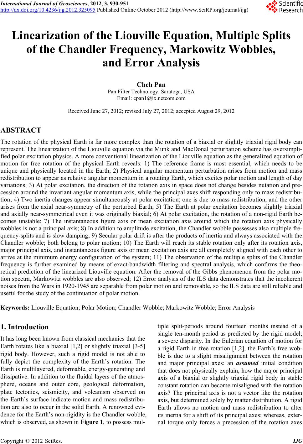
|