Journal of Information Security, 2012, 3, 245-250
http://dx.doi.org/10.4236/jis.2012.34031 Published Online October 2012 (http://www.SciRP.org/journal/jis)
Unsupervised Multi-Level Non-Negative Matrix
Factorization Model: Binary Data Case
Qingquan Sun1, Peng Wu2, Yeqing Wu1, Mengcheng Guo1, Jiang Lu1
1Department of Electrical and Computer Engineering, The University of Alabama, Tuscaloosa, USA
2School of Information Engineering, Wuhan University of Technology, Wuhan, China
Received July 21, 2012; revised August 26, 2012; accepted September 7, 2012
ABSTRACT
Rank determination issue is one of the most significant issues in non-negative matrix factorization (NMF) research.
However, rank determination problem has not received so much emphasis as sparseness regularization problem. Usu-
ally, the rank of base matrix needs to be assumed. In this paper, we propose an unsupervised multi-level non-negative
matrix factorization model to extract the hidden data structure and seek the rank of base matrix. From machine learning
point of view, the learning r esult depends on its pr ior knowledg e. In our unsuperv ised multi-level model, we construct a
three-level data structure for non-negative matrix factorization algorithm. Such a construction could apply more prior
knowledge to the algorithm and obtain a better approximation of real data structure. The final bases selection is
achieved through L2-norm optimization. We implement our experiment via binary datasets. The results demonstrate that
our approach is able to retrieve the hidden structure of data, thus determine the correct rank of base matrix.
Keywords: Non-Negative Matrix Factorization; Bayesian Model; Rank Determination; Probabilistic Model
1. Introduction
Non-negative matrix factorization (NMF) was proposed
by Lee and Seung [1] in 1999. NMF has become a
widely used technique over the past decade in machine
learning and data mining fields. The most significant
properties of NMF are non-negative, intuitive and part
based representative. The specific applications of NMF
algorithm include image recognition [2], audio and acou s-
tic signal processing [3], semantic analysis and content
surveillance [4]. In NMF, given a non-negative dataset
M
N
VR

, the objective is to find two non-negative fac-
tor matrices
M
K
WR and
K
N
H
R 
..0, 0VW
HstW H

. Here W is
called base matrix and H is named feature matrix. In ad-
dition, W and H satisfy
(1)
K is the rank of base matrix and it satisfies the inequality
K
MN MN.
For NMF research, the cost function and initialization
problems of NMF are the main issues for researchers.
Now the rank determination problem becomes popular.
The rank of base matrix is indeed an impor tant parameter
to evaluate the accuracy of structure extraction. On the
one hand, it reflects the real feature and property of data;
on the other hand, more accurate learning could help us
get better understanding and analyzing of data, thus im-
proving the performance in applications: recognitio n [5,6]
surveillance and tracking. The main challenge of rank
determination problem is that it is p re-defined. Therefore,
it is hard to know the correct rank of base matrix before
the updating process of components. As the same as the
cost function, there are no more priors added to the algo-
rithm in previous methods. That is why the canonical
NMF method and traditional probabilistic methods (ML,
MAP) cannot handle the rank determination problem.
Therefore in this paper, we propose an unsupervised
multi-level model to automatically seek the correct rank
of base matrix. Furthermore, we use L2-norm to show the
contribution of hyper-prior in correct bases learning pro-
cedure. Experimental results on two binary datasets dem-
onstrate that our method is efficient and robust.
The rest of this paper is organized as follows: Section
2 provides a brief review of related works. In Section 3,
we describe our unsupervised multi-level NMF model in
details. The experimental results of two binary datasets
are shown in Section 4. Section 5 concludes the paper.
2. Related Work
As we mentioned above, rank determination problem is a
new popular issue in NMF research. Actually, there are
few literatures discussing this issue. Although the author
in [7] proposed a method based on sampler selection, it
C
opyright © 2012 SciRes. JIS

Q. Q. SUN ET AL.
246
needs to pass through all the possible values of rank of
base matrix to choose the best one. Obviously, this method
is not impressive enough for unsupervised learning. In
[8], the author proposed a rank determination method
based on automatic relevan ce determination. In this m e t hod,
a parameter is defined relevant to the columns of W.
Then using EM algorithm to find a subset, however, this
subset of bases is not accurate to represent true bases.
Actually, the nature of this hyper-parameter is to affect
the updating procedure of base matrix and f eature matrix,
thus affect the components’ distributions.
The only feasible solution is fully Bayesian models.
Such kind of methods have been proposed in [9]. In this
paper, the author addresses an EM based fully Bayesian
algorithm to discover the rank of base matrix. EM based
methods are an approximation solution. In comparison, a
little more accurate solution is Gibbs sampling based
methods. Such approach is utilized to find the correct
rank in [10]. Although such kinds of methods are flexible,
it requires successively calculation of the marginal like-
lihood for each possible value of each rank K. The
drawback is too much computation cost involved. Addi-
tionally, when such methods are applied to real time ap-
plication or some large scale dataset based applications,
the high computation load is impractical. Motivated by
the current condition, we propose a low computation,
robust multi-level model for NMF to solve rank deter-
mination problem. Our unsupervised model with multi-
lever priors only calculate once of the rank of base ma-
trix and is able to successfully find the correct rank of
base matrix given a large enough rank K. Therefore, our
method involves less computation. This will be discussed
in details in next section.
3. Unsupervised Multi-Level Non-Negative
Matrix Factorization Model
In our unsupervised multi-level NMF model, we intro-
duce a hyper-prior level. Hence, there are three levels in
our model: data model, prior model, hyper-prior model.
The model structure is shown in Figure 1. We will seek
Figure 1. Unsupervised multi-level non-negative matrix fac-
torization model.
the solutions through optimizing the maximum a poste-
rior criterion. Our approach could be depicted by the
following equation, here c

denotes equality up to a
constant,

is the prior of both W and H.








,, loglog
log log
c
MAPp p
pp





WHVWH W
H (2)
The difference between our approach and the tradi-
tional MAP criterion is that in traditional one there is no
hyper-prior added to the model. Moreover, in our model
we attempt to update the hyper-priors recursively, but not
just set it as a constant.
3.1. Model Construction
In NMF algorithm, the updating rules are based on the
specific data model. Therefore, the first step is to set a
data model for our problem. Here, in our experiment we
assume that the data follows Poisson distribution. Con-
sequently, the cost function of our model will be gener-
alized KL-divergence. So given a variable x, which fol-
lows Poisson distribution with parameter

, we have




1
x
px ex




. Thus, in NMF algorithm,
given dat a s et V, we have the likelihood


 
1pe



V
WH
VWHWHV (3)
The generalize d KL-divergence is given by:

 
log mn
KLmnmn mn
mn mn
v
Dv vwh
wh



 





VWH(4)
Thus, the log-likelihood of the dataset V can be re-
written as:




log
1loglog1
KL
mn mnmn
mn
p
D
vv v



 


VWH
VWH (5)
From (2) and (5) we could conclude that maximizing a
posterior is equivalent to maximizing the log-likelihood,
and maximizing the log-likelihood is equivalent to mini-
mizing the KL-divergence. Thus, maximizing a posterior
is equivalent to minimizing the KL-divergence. Therefore,
it is possible to find a base matrix W and a feature matrix
H to approximate the dataset V via maximizing a poste-
rior criterion.

In data model

pVWH we regard WH as the pa-
rameter of data V. With respect to the base matrix W and
the feature matrix H, we also introduce a parameter

as a prior to them. Moreover, we define an independent
Exponent distribution for each column of W and each
row of H with prior k

because exponent distribution
has sharper performance. It is no doubt that we can
choose other exponential family distributions such as

Q. Q. SUN ET AL. 247
Gaussian distribution, Gamma distribution, etc. There-
fore, the columns of W and rows of H yield:

kmk
w
pw e




mk k k (6)

kn k
ph kkn
h
ke



 (7)
Then the log-likelihood of the priors cou
te ld be rewrit- n as:



kkmk
pw    (8) log log
mk
  W

log log
kn
  H
Compare to setting

kkkn
ph    (9)

as a constant, the diversity of
k

and recursively updting of k a

enable the inference
ocedure to converge at the stationary point. Through
calculating the L2-morm of each column of base matrix
W, we could discover that the data finally emerges to two
clusters. One cluster contains the points of which the
L2-norm are much larger than 0, whereas in the other
cluster the L2-norm values are 0 or almost 0.
In order to find the best value for k
pr

, here we intro-
duce hyper-prior for k

. Since k

ishe parameter of
Exponent distributione defink
t
e , w

follows Gamma
distribution which is the conjugaterior for Exponent
distribution. p


,e
xp
kk
b   (10)
k kr-priors of k
1
1
() k
a
kkk k
a
k
pab ab 


Here a and b are the hype

. Thus,
thoe log-llihood f ike

is given as:

 
og kkk
b
 (11)
3.2. Inference
hment of data model and the deduction
log p 
loglog1 l
kkk k
kab a a 
After the establis
of log-likelihood of each prior, we can gain the maxi-
mum a posterior equation:


 




 
log1 log1
log
log
loglog1 log
mn mnmn
mn
KLk mkk
mk
kkn k
kn
kkkkk kk
k
vv v
Dw
h
aba bab




 





 

 
,,MAP


VW
H(12)
Since the first factor in (12) has nothing to do with the
pri
 WH
ors, and we have discussed the relationship between
the posterior probability and KL-divergence, here we
minimize the second factor to seek the solutions for this
criterion. In our paper, we choose gradient decent updat-
ing method as our updating rule. Although multiplicative
method is simpler, it has no detailed deduction about
why the approach works. On the contrary, gradient de-
cent updating will give us clear deduction about the
whole updating procedure. We utilize this method to in-
fer the priors W and H, as well as the hyper-priors

and b. First we find the gradient of the parameters:
TT
f
W




VHH
WH (13)
TT
f
H


 


V
WW
WH (14)

11
mkkn kk
mn
k
fwhbNMa




 (15)
2
kk
kk k
a f
bb b
  
 (16)
Then we utilize gradient coefficient to get rid of the
subtraction operation during the updating procedure for
W and H to guarantee the non-negative constrain. The
parameters k

and k b are updated by zeroing.
The updating rules listed as follows: are

mn
vkn
n
mn
mk mk kn k
n
h
wh
ww h







 (17)

mn
mk
mmn
kn knmk k
m
v
wwh
hh w




 

 (18)
1
1
k
kmkkn k
mn
MNa
whb




 (19)

k
kk
a
b


 (20)
Then we find the correct bases and determine the order
of the data model by:
1
RB (21)
where B is defined as


22
,0
kk
ww
(22)
R is the rank of base matrix.
4. Experimental Results and Evaluation
B
In this section, we apply our unsupervised multi-level
NMF algorithm on two binary datasets. One is fence
dataset, and the other is famous swimmer dataset. Both
of the experiment results demonstrate the efficacy of our
method on the rank determination issue.

Q. Q. SUN ET AL.
248
4.1. Fence Dataset
We first performed our experiments on fence dataset.
f
ra
Here I defined the data with four row bars (the size is 1 ×
32) and four co lumn bars (the size is 32 × 1). The size of
each image is 32 × 32 with zero-value background, and
the value of each pixel in eight bars is one. Each image is
separated into five parts in both horizontal direction and
vertical direction. Additionally, in each image the num-
ber of row bars and the number of column bars should be
the same. For instance, there are two row bars in a sam-
ple image, then there should be two column bars in this
image. Hence, the total number of the fence dataset is N =
69. The samples of Fence dataset are shown in Figure 2.
Here, we set the initial rank K = 16 (the initial value o
nk K needs to be larger than the value of real rank of
base matrix), the hyper-parameter a = 2,


1
0.05 0.05
k
K
b . Figure 3 shows t
learned via our unsupervised multi-
level NMF approach, we could see that the data is sparse,
especially the base matrix. In both images, the color parts
denote the effective bases or features, and the black parts
denote irrelevant bases or features there. In addition,
from image processing perspective, we can conclude that
compared to the values of effective bases and features,
the values of irrelevant bases and features are very small,
since the color of such pixels are very dark. We could
clearly find that there are eight color column vectors in
the first image. Additionally, among the eight color vec-
tors, four are composed of several separated color pixels,
whereas the other four are composed of assembly pixels.
Actually, the former four vectors are row bars, and the
latter four vectors are column bars. We resize the dataset
in columns during factorization procedure. Hence the
row bars and column bars have different structures. Fur-
thermore, there are also eight rows in the second image,
which are the corresponding coefficients of the bases.
he base matrix
ure matrix and feat
Figure 2. Sample images of fence dataset.
Figure 3. Base matrix W anature matrix H learned via
how the bases clearly, we draw the bases
in
4.2. Swimmer Dataset
tial rank is set to K = 25,
th
d fe
our algorithm.
In order to s
Figure 4. Since we set the initial rank of base matrix K =
16, however, only eight images have non-zero values.
Moreover, the eight images show 4 row bars and 4 col-
umn bars appearing in different positions. The results are
perfectly consistent to the design of Fence dataset.
Therefore, we could get the conclusion that our algorithm
is very powerful and efficient to find the real basic com-
ponents and the correct rank.
The other dataset we used is the swimmer dataset.
Swimmer dataset is a typical dataset for feature extrac-
tion. Due to the clearly definition and composition of 16
dynamic parts, it is quite appropriate to the unique char-
acteristic of NMF algorithm, which is to learn part-based
data. As we know, however, the swimmer dataset is a
gray-level image dataset. In our experiment, we focus on
binary dataset, so first we need to convert this gray-level
dataset to binary dataset. Then apply our approach to
perform inference. In this swimmer dataset, there are 256
images totally, each of which depicts a swimming ges-
ture using one torso and four dynamic limbs. The size of
each image is 32 × 32. Each dynamic part could appear
at four different positions. Figure 5 shows some sample
images of the swimmer dataset.
In this experiment part, the ini
e initial values of hyper-parameters are a = 2,


1
0.05 0.05
k
K
b

. Figure 6 shows the experiment
Figure 4. The bases obtained by our algorithm on fence
dataset.
Figure 5. Sample images of the swimmer dataset.

Q. Q. SUN ET AL. 249
resul
ages and the
co
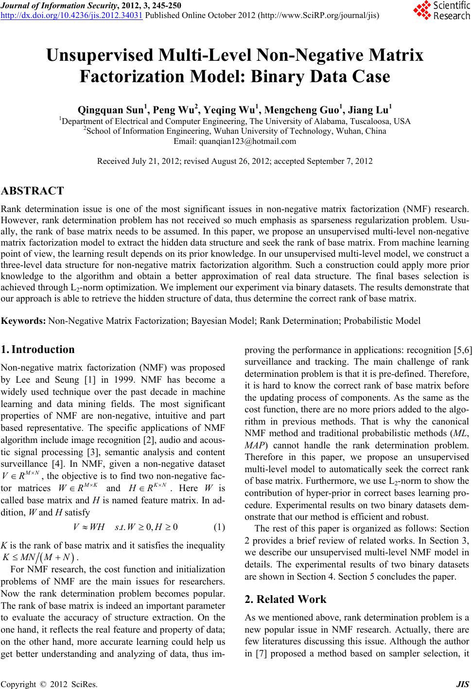
ts for the swimmer dataset. It could be observed that
as for this dataset, we also could find out the correct
bases via our algorithm. In this figure there are 25 base
images. The black ones correspond to irrelevant bases,
and the other 17 images depict the torso and the limbs at
each possible position. We can see that the correct torso
and limbs are discovered successfully.
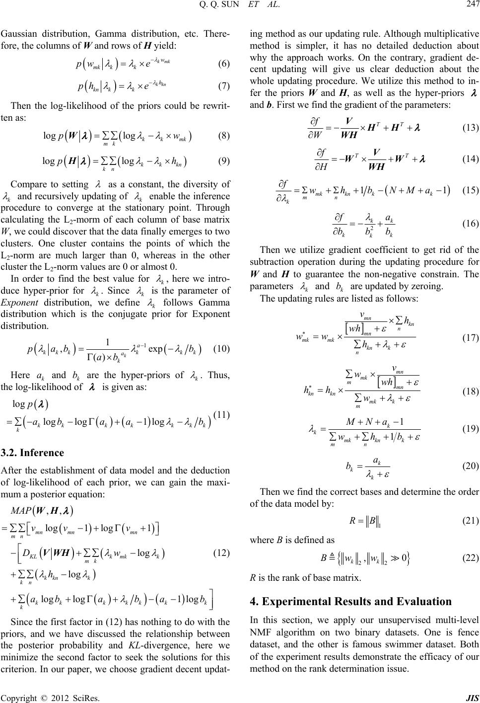
The differences between the black im
rrect base images are shown in Figure 7. Figure 7
depicts L2-norm of each column of the base matrix. The
total number of points in this figure is the same to the
initial rank. Obviously, the points are classified into two
clusters. One is zero-value cluster, and the other is lar-
ger-value cluster. Thus the rank of base matrix in swim-
mer dataset is 117RB. The results of L2-norm of
base matrix not ow we could find the correct
bases, but also tell us how we could determine the correct
rank of base matrix.
only tell us h
Figure 6. The bases of swimmer dataset learned by our al-
gorithm.
05 10 15 20 25
0
0.1
0.2
0.3
0.4
0.5
0.6
0.7
0.8
0.9
1
Base ve ctor inde
x
Norm alized L2 nor m
Normalized L
2
norm
Figure 7. L2-norm of base vectors.
supervised multi-level non-
[1] D. D. Lee andhe Parts of Objects
5. Conclu
We have presented an un
sion
negative matrix factorization algorithm which is power-
ful and efficient to seek the correct rank of a data model.
This is achieved by introducing a multi-prior structure.
The experiment results on binary datasets adequately
demonstrate the efficacy of our algorithm. Compare to
the fully Bayesian method, it is simpler and more con-
venient. The crucial points of this method are how to
introduce the hyper-priors and what kind of prior is ap-
propriate to a certain data model. This algorithm also
could be extended to other data models and noise models.
Although our experiment is based on binary dataset, this
algorithm is suitable to other datasets such as gray-level
dataset, colorful dataset, etc.
REFERENCES
H. S. Seung, “Learning t
by Non-Negative Matrix Factorization,” Nature, Vol. 401,
No. 6755, 1999, pp. 788-791. doi:10.1038/44565
[2] Z. Yuan and E. Oja, “Projective Non-Negative Matrix
urrieu, “Non-Negative
Factorization for Image Compression and Feature Extrac-
tion,” Springer, Heidelberg, 2005.
[3] C. Fevotte, N. Bertin and J. L. D
Matrix Factorization with the Itakura-Saito Divergence,”
With Application to Music Analysis. Neural Computation,
Vol. 21, No. 3, 2009, pp. 793-830.
doi:10.1162/neco.2008.04-08-771
[4] M. W. Berry and M. Browne, “Email Surveillance Using
Non-Negative Matrix Factorization,” Computational and
Mathematical Organization Theory, Vol. 11, No. 3, 2005,
pp. 249-264. doi:10.1007/s10588-005-5380-5
[5] Q. Sun, F. Hu and Q. Hao, “Context Awareness Emer-
ile Targets Region-of-
“Clustering-
06
gence for Distributed Binary Pyroelectric Sensors,” Pro-
ceeding of 2010 IEEE Conference on Multisensor Fusion
and Integration for Intelligent Systems, Salt Lake City,
5-7 September 2010, pp. 162-167.
[6] F. Hu, Q. Sun and Q. Hao, “Mob
Interest via Distributed Pyroelectric Sensor Network:
Towards a Robust, Real-Pyroelectric Sensor Network,”
Proceeding of 2010 IEEE Conference on Sensors, Wai-
koloa, 1-4 November 2010, pp. 1832-1836.
[7] Y. Xue, C. S. Tong and Y. C. W. Chen,
Based Initialization for Non-Negative Matrix Factoriza-
tion,” Applied Mathematics and Computation, Vol. 205,
No. 2, 2008, pp. 525-536.
doi:10.1016/j.amc.2008.05.1
utomatic Rank Determi-
ative Ma-
[8] Z. Yang, Z. Zhu and E. Oja, “A
nation in Projective Non-Negative Matrix Factorization,”
Proceedings of 9th International Conference on LVA/ICA,
St. Malo, 27-30 September 2010, pp. 514-521.
[9] A. T. Cemgil, “Bayesian Inference for Non-Neg
trix Factorization Models,” Computational Intelligence
and Neuroscience, Vol. 2009, 2009, Article ID: 785152.
doi:10.1155/2009/785152
[10] M. Said, D. Brie, A. Mohammad-Djafari and C. Cedric,

Q. Q. SUN ET AL.
250
“Separation of Nonnegative Mixture of Nonnegative
Sources Using a Bayesian Approach and MCMC Sampl-
ing,” IEEE Transactions on Signal Processing, Vol. 54,
No. 11, 2006, pp. 4133-4145.
doi:10.1109/TSP.2006.880310