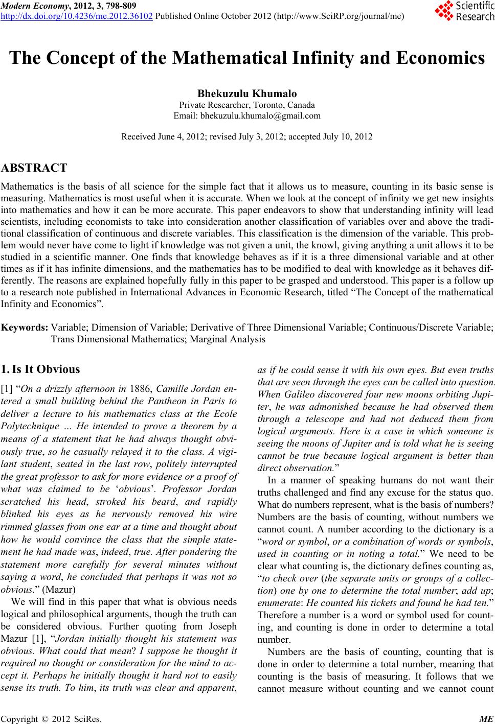Modern Economy, 2012, 3, 798-809
http://dx.doi.org/10.4236/me.2012.36102 Published Online October 2012 (http://www.SciRP.org/journal/me)
The Concept of the Mathematical Infinity and Economics
Bhekuzulu Khumalo
Private Researcher, Toronto, Canada
Received June 4, 2012; revised July 3, 2012; accepted July 10, 2012
ABSTRACT
Mathematics is the basis of all science for the simple fact that it allows us to measure, counting in its basic sense is
measuring. Mathematics is most useful when it is accurate. When we look at the concept of infinity we get new insights
into mathematics and how it can be more accurate. This paper endeavors to show that understanding infinity will lead
scientists, including economists to take into consideration another classification of variables over and above the tradi-
tional classification of continuous and discrete variables. This classification is the dimension of the variable. This prob-
lem would never have come to light if knowledge was not given a unit, the knowl, giving anything a unit allows it to be
studied in a scientific manner. One finds that knowledge behaves as if it is a three dimensional variable and at other
times as if it has infinite dimensions, and the mathematics has to be modified to deal with knowledge as it behaves dif-
ferently. The reasons are explained hopefully fully in this paper to be grasped and understood. This paper is a follow up
to a research note published in International Advances in Economic Research, titled “The Concept of the mathematical
Infinity and Economics”.
Keywords: Variable; Dimension of Variable; Derivative of Three Dimensional Variable; Continuous/Discrete Variable;
Trans Dimensional Mathematics; Marginal Analysis
1. Is It Obvious
[1] “On a drizzly afternoon in 1886, Camille Jordan en-
tered a small building behind the Pantheon in Paris to
deliver a lecture to his mathematics class at the Ecole
Polytechnique … He intended to prove a theorem by a
means of a statement that he had always thought obvi-
ously true, so he casually relayed it to the class. A vigi-
lant student, seated in the last row, politely interrupted
the great professor to ask for more evidence or a proof of
what was claimed to be ‘obvious’. Professor Jordan
scratched his head, stroked his beard, and rapidly
blinked his eyes as he nervously removed his wire
rimmed glasses from one ear at a time and thought about
how he would convince the class that the simple state-
ment he had made was, indeed, true . After pondering the
statement more carefully for several minutes without
saying a word, he concluded that perhaps it was not so
obvious.” (Mazur)
We will find in this paper that what is obvious needs
logical and philosophical arguments, though the truth can
be considered obvious. Further quoting from Joseph
Mazur [1], “Jordan initially thought his statement was
obvious. What could that mean? I suppose he thought it
required no thought or consideration for the mind to ac-
cept it. Perhaps he initially thought it hard not to easily
sense its truth. To him, its truth was clear and apparent,
as if he could sense it with his own eyes. But even truths
that are seen throug h th e eyes can be ca lled into qu e stion.
When Galileo discovered four new moons orbiting Jupi-
ter, he was admonished because he had observed them
through a telescope and had not deduced them from
logical arguments. Here is a case in which someone is
seeing the moons of Jupiter and is told wha t he is seeing
cannot be true because logical argument is better than
direct observation.”
In a manner of speaking humans do not want their
truths challenged and find any excuse for the status quo.
What do numbers represent, what is the basis of numbers?
Numbers are the basis of counting, without numbers we
cannot count. A number according to the dictionary is a
“word or symbol, or a combination of words or symbols,
used in counting or in noting a total.” We need to be
clear what counting is, the dictionary defines counting as,
“to check over (the separate units or groups of a collec-
tion) one by one to determine the total number; add up;
enumerate: He counted his tickets and found he had ten.”
Therefore a number is a word or symbol used for count-
ing, and counting is done in order to determine a total
number.
Numbers are the basis of counting, counting that is
done in order to determine a total number, meaning that
counting is the basis of measuring. It follows that we
cannot measure without counting and we cannot count
C
opyright © 2012 SciRes. ME

B. KHUMALO 799
without numbers. Being able to count, 2 cups, 3 baskets,
6 antelope, we are basically measuring. Every culture,
humans to survive need a basic pattern to recognize a
way to measure, two moons ago, my stomach is full be-
cause I ate so much of an antelope. Then a human be-
cause they can measure will understand portions, not the
whole leg, but if you divide that leg into 5 equal parts,
one of those parts will fill me up. From counting we can
understand portions, very important because how else
would humans share and reward each other. A portion is
a measurement.
Measurement is the basis of scientific thought, so
much iron plus so much titanium and the alloy will be so
strong, GNP is equal to so much is basically a tally,
counting, what others think as more sophisticated meth-
ods of counting, but counting nonetheless. Counting is
counting be one using fingers or fancy notation. One
sitting in an air conditioned office in downtown Manhat-
tan counting billions of dollars in revenue is no different
from a Babylonian merchant, or Mwenemutapa merchant
in ancient times counting his revenue, or a Cavemen
counting an antelope herd, they are all taking a tally, it is
just counting.
Given that numbers arose from our need to measure,
once they existed they existed. It is when people settled
down that they had time to do something more with
numbers. Quoting from Dirk Struik [2], “little progress
was made in understanding numerical value and space
relations until the transition occurred from the mere
gathering of food to its actual production, from hunting
and fishing to agriculture … Fisherman and hunters
were in large part replaced by primitive farmers. Such
farmers remaining in one place as long as the soil was
fertile, began to build more permanent dwellings …”
This is not a paper on mathematical history, but hope-
fully one understands that with settlements people had
time to look more carefully at the numbers and find rela-
tionships between numbers, multiplication instead of
addition, then division, things that nomads would not
have for example found the time for.
With more understanding of relationships the notation
could become more abstract, but was accepted as long as
it was logically sound. Take the relationship a + b = c. It
is just a relationship and breaks no laws of logic or
mathematics. a and b can be any numbers, and their sum
is equal to c. But though very abstract, the relationship
still represents just counting, one is tallying a and b.
All mathematical relationships essentially, in one way
or another, represent measuring, r2 = A is the area of a
circle, this is a relationship between  and r, where  is pi,
r is the radius of the circle and A is the area of the circle.
R, the radius of the circle, is not limited, it can be 1 cm or
1 billion km, but we can get to the area because we un-
derstand the relationship that determines the area of a
circle. It is here for example that we enter into the di-
lemma of infinity. The area of a circle is being used here
because it is assumed that anybody capable of reading
and deciphering this paper was taught this relationship in
their early teenage years. But first let us make sure we
understand the concept of infinity in the mathematical
sense.
2. Cantor’s Logic
[3] “It was Georg Cantor, a Russian-German mathema-
tician, who resolved these seeming paradoxes that cir
cled the notion of infinity. It was a brilliant piece of work.
He defined infinity through infinite collections. Such col
lections were characterized by the fact that you could
subtract a finite number of elements from them without
changing the size of the collection. You could even sub-
tract an infinite numb er …” (Kaplan)
Cantor’s logic was unique and correct, this paper does
not seek in any manner to even suggest Cantor was
wrong, he was right. The paper merely seeks to make
clear the application of Cantor’s logic in the practical
rather than in the abstract where Cantor’s logic remains.
Cantor’s logic is great even today [3], “This proof—as
simple and subtle as a ll great art—throws open the gates
to what Hilbert called Cantor’s paradise.” (Kaplan).
Being simple it is easy to understand.
The application of Cantor’s logic outside the abstract
can be found in Cantor’s thought and how he saw the
world, in particular how the concepts of the continuum
was looked at. [4] “Basic to the progress of all science,
he felt was an acceptable concept of continuity. It’s na-
ture and properties had always stimulated passionate
controversy and great differences of opinion, though he
was certain that the roots of were east to identify. Un-
derlying the concept of the continuum, different features
had always been stresses, but no exact or complete defi-
nition had ever been given. He assigned original blame
to the Greeks, who had been the first to study the prob-
lem but in such ambiguous terms that myriad interpreta-
tions were left open to later doxographers and commen-
tators. For example, Cantor believed that Aristotle and
Epicurus represented polar opposites on the subject of
the continuum and its consistency. On the one hand, Ar-
istotle and his followers believed in a continuum com-
posed of parts which were divisible without limit. Epicu-
rus by contrast, developed the atomist position and re-
garded the continuum as somehow synthesized from atom
which were imagined as finite entities.” (Dauben)
Cantor did not agree with those who wanted a middle
ground between the two, though at the end though Cantor
would have been loath to agree, Cantor ultimately was
closer to Aristotle than he was to Epicurus, though ulti-
mately he agreed with neither. He for example did not

B. KHUMALO 800
agree with Aristotle’s viewpoint that infinite numbers
could “annihilate” finite numbers.
Cantor’s proof is widely accepted, but there are always
those dissenters though few in number who do not agree
with Cantor’s proof. [5] “Mathematicians feel that
mathematical existence is established only when one of
the objects whose existence is in question is actually
constructed and exhibited. The above proof does not es-
tablish the existence of transcendental numbers by pro-
ducing a specific example off such a number.” (Eves).
Transcendental numbers are non algebraic numbers.
Though Cantor did not come up with such a number his
theory was proved in a logical and systematic manner.
To understand Cantor’s logic it would be wise to read the
book by the Kaplan couple entitled, “The art of the Infi-
nite.”
3. Is Infinity Practical Outside Pure
Mathematics
Cantor might have came out with an acceptable proof of
infinity, one should read Chapter nine of the book, “The
Art of the Infinite”. At the beginning of the Chapter the
authors quote Galileo, [3] “In 1638 Galileo argued that
“equal”, “greater”, and “less” can’t apply to infinite
quantities because a line segment contains an infinity of
points, so a longer line segment would have to contain
more than that infinity, which is impossible.” Cantor
would disprove this line of thinking by using set theory,
sets of infinity within infinity, but infinity posses huge
dilemma’s outside pure mathematics that Galileo perhaps
was possibly anticipating, maybe often, equal, greater
and less cannot apply to ‘infinite’ quantities.
A twelve year old or even a six year old with reason-
able mathematical abilities understands that numbers go
on forever and any number followed by a decimal also
goes on for ever, for example we can have
0.134. ···9···n··· just as numbers run from 1, 2, 3 ··· n···,
n being a very large number. Technically speaking, a
radius of a circle can for example be 1 m, 1.5 m, 1.5333
m, 1.533336777···m depending on the accuracy of our
measuring instruments, what is important is that it is pos-
sible. Therefore r follows the logic established by Cantor,
r can be divided into infinite parts after the decimal for
example. The radius say it falls between 1 and 2 m or cm,
it can be for exams 1.5 cm or 1.59 cm or 1.599···cm, this
cannot be debatable.
Throwing a stone in the air, it will return to the ground.
[6] We can for example with proper instruments know
how far the stone is from the ground as illustrated in
Figure intro.
Does the concept of infinity hold in the example of the
stone, say the stone is of the ground for n seconds. The
stone after all cannot logically be of the ground for ever,
0 n
Time
Figure intro: Throw i ng stone from ground.
there is the force of gravity therefore n, the number of
seconds that the stone is off the ground cannot be forever
whilst the radius of a circle can logically be infinitely
large or at the least as big as the universe, a stone how-
ever will normally come down in a matter of seconds,
therefore logically speaking n cannot be infinitely large.
Let us say that n is 4 seconds, therefore at anytime be-
tween 0 and 4 seconds the stone is off the ground and in
motion. It follows that at 3 seconds the stone is still in
motion even at 3.9 seconds or 3.999, 3.99999, or
3.999··· seconds the stone is still in motion. It follows
that Cantor’s logic holds with the stone been thrown in
the air. The stone is in constant motion until it hits the
ground after n seconds, however each second that it is in
the air can be split into as many parts as instrumentation
allows us to measure, at 2.5 seconds the stone is off the
ground, at 2.51 seconds the stone is of the ground, at
2.511, 2.5111, 2.51111... seconds the stone is still of the
ground and seconds logically can be split into infinite
parts. Time is truly a continuous phenomenon and like
distance can be broken into infinite parts. It is the quality
of the continuous that allowed calculus to be discovered.
Reading Dewdney’s book “A Mathematical Mystery
Tour”, one will understand the logic of how Leibniz dis-
covered calculus. Some claim Newton discovered calcu-
lus but hid it for twenty years, but that is for Newton’s
defenders, why hide your work and when somebody else
publishes their work claim to already know that. When
Leibniz discovered calculus he could do so because of
the nature of the continuous.
By seeing how far the stone is off the ground, with
calculus we can see the rate of change, that is to say the
velocity of the stone in this case. It works perfectly be-
cause time follows Cantor’s logic and can be divided into
infinite parts. Therefore at 2.2 seconds we can know the
rate of change of the stone, to be more specific the veloc-
ity as well as at 2.22 or 2.2267788 seconds we can know
the rate of change of the stone because of the nature of
time 2.2267788 seconds does exist logically and practi-
cally. In fact differential calculus is very important in
today’s world. [7] “The new calculus came to be applied
to just about every conceivable type of motion or change

B. KHUMALO 801
in the ph ysical wo rld . Often math ema ticians or ph ysicists
would begin with an equation that involved differentials,
moving by integration to an actua l formu la of positio n, ...
Such equations called “differential equations”, have
dominated physics ever since. They appear in Schrod-
inger’s equation of the hydrogen atom and in Einstein’s
theory of general relativity.” (Dewdney)
The “new calculus” came to be applied to just about
every conceivable type of motion or change because the
changes being measured were/are seemingly instantane-
ous, this seemingly instantaneous change is supported by
and itself supports Cantor’s assertions on the concepts of
the mathematical infinity. A stone thrown in the air and
in 4 seconds hits the ground again it will be in motion in
2 seconds, it will be in motion in and at all parts between
2 and 3 seconds, because seconds can be broken into
infinite parts. This seemingly instantaneous change de-
pends on a large part on the unit.
4. The Unit
Cantor’s abstract conceptualization of the infinite seem-
ingly defended the non abstract concept of a stone
thrown into the air. Truly understanding the abstract con-
cept laid down by Cantor is itself stretching the imagina-
tion, but often it is easily applied in the real world. That
between 0 and 1 there are infinite numbers as well be-
tween 0 and 0.1. Between each real number there is a set
of infinite sets, countless, but can this affirmation always
be applied in the real world.
Take a piece of wood say 10 cm wide, 10 cm high, and
3 meters long. It is cut into two pieces, each piece 10 cm
wide, 10 cm high but different lengths. One is 2 meters
long the others is 1 meter long. Using Cantor’s abstract
conceptualization that say there are infinite parts between
0 and 1, 0 and 2, and, 0 and 3, infinity is everywhere in
Cantor’s abstract, seemingly true with the variables such
as time and distance but can it be true when we cut the
two wood blocks above that have same height, and width
but different lengths. Wood is basically made up of mo-
lecules. It follows that the larger block of wood has more
molecules than the smaller block of wood, though the
molecules are similar since the two blocks where origi-
nally one block that was cut into two blocks of varying
sizes. The larger block has to have more molecules and
they have to be a finite number, therefore Cantor’s ab-
stract conceptualizations do not hold in this case. You
can not break the molecules into infinite parts, once the
molecules are broken it is no longer wood.
The illustration above regarding wood does not follow
Cantor’s mathematical abstraction of infinity in two very
specific ways:
1) With the wood the larger block has more parts, (the
basic part being a molecule), than the smaller block;
2) Both blocks being built by molecules have finite
parts that they can be broken down to.
The logic that there are infinite parts breaks down in
the reality where molecules of wood are concerned for
example.
5. Why Cantor’s Mathematical Infinity
Often Fails in the Material
Why Cantor’s abstraction often fails is because of the
nature of the material, for this it will be easier understand
if we go and understand an acceptable scientific theory
concerning the beginnings of the universe, we must go to
the “Big Bang” theory. “The Big Bang theory is an effort
to explain what happened at the very beginning of our
universe. Discoveries in astronomy and physics have
shown beyond a reasonable doubt that our universe did in
fact have a beginning. Prior to that moment there was
nothing; during and after that moment there was some-
thing: our universe [8] ... According to the standard the-
ory, our universe sprang into existence as ‘singularity’
around 13.7 billion years ago ... The pressure is thought
to be so intense that finite matter is actually squished into
infinite density.” (All About Science). The usually cliché
is that the universe started as a small dot, what is impor-
tant is the matter was finite contained in that small dot.
There is so much matter in the universe, the matter might
be transformed but it remains finite. One of the first real
lessons one learns in science is that energy cannot be
destroyed only transformed, you cannot increase the
amount of energy in the universe, because it is finite, all
those many billions of years ago contained in a small
“dot”.
Assuming all the energy in the universe amounted to N,
you therefore cannot have more than or less than N
amounts of energy. However one can count to N + 1, or
N + 100, but N + 1 and N + 100 are just abstractions, the
universe cannot have that amount of energy, there is a
limit, just as a piece of wood is limited into how much it
can be broken down, one will end up smashing mole-
cules and atoms and getting completely different materi-
als.
The universe might be expanding but it has finite en-
ergy and therefore how much matter it can contain and
matter cannot always be broken into infinite parts. Num-
bers were invented by human beings to aide counting and
measuring, that we can find relationships in numbers
aides in the measuring process. But because of nature
itself we cannot apply the same logic to every variable in
those relationships. Some variables will follow the logic
of the infinite as expressed in mathematics and devel-
oped by Cantor, variables like time, some will not, vari-
ables like wood.
Independent variables that follow Cantor’s obvious

B. KHUMALO 802
logic, that is to say can be broken into infinite parts such
as time, distance, been able to be broken into infinite
parts can have change that is seemingly instantaneous in
say differential calculus. Change from 3 seconds to 4
seconds for example is meaningless, because there is
something occurring at 3.5 seconds, 3.6 seconds, 3.9
seconds, 3.99... seconds, the rate of change because of
the nature of an independent variable such as time can be
measured at exactly or near exactly 4 seconds.
What however is the rate of change say not if the in-
dependent variable is not so divisible, that is to say can-
not be broken into infinite parts like time, or distance,
what if the independent variable is addition of atoms of a
certain element adding them from 3 to 4. We cannot have
3.99... atoms, or 3.5 atoms it is illogical, Cantor’s logic
cannot hold, the instantaneous change has a different
meaning, in the case of the atom because it is an indivisi-
ble variable, the instantaneous change is the resultant
change from 3 atoms to 4 atoms.
In economics a major variable is labor, add so much
labor and output increases by so much for example. La-
bor is not like time or liters that can be broken into infi-
nite parts, a human is just that a human, we cannot have
half a laborer, a laborer cannot be broken into parts let
alone infinite parts. How then can the formulae/differen-
tial calculus for rate of change for labor output where the
variable labor cannot be broken into infinite parts, be the
same as when time is the independent variable, whilst
time can be broken into infinite parts, it should be obvi-
ous that the differential calculus needs to be modified.
The calculus invented by Gottfried Wilhelm Leibniz
needs to be modified to deal with variables that cannot be
broken into infinite parts. If the variable can be broken
into infinite parts like time, there is without doubt no
need to modify Leibniz’s work. It is mandatory to make
these changes otherwise independent variables be they be
able to be broken into infinite parts or not are being
treated the same, that is misguided logic.
Before moving further let us go back to the indivisible
atom and indivisible laborer. Now there are people who
will talk of atoms been divided and broken up, the atom
bomb and nuclear power stations being the great exam-
ples, however when atoms are broken up they become
different elements, in theory if one for example had a
way to add or subtract protons, neutrons and electrons
they could literally create water from uranium, gold from
lead, but adding or subtracting protons, neutrons, and
electrons creates a different isotope or element.
Returning to the indivisible laborer and atom, the cal-
culus discovered by Leibniz has shortcomings if such
variables were independent variables, however that can-
not be true if they are dependent variables. If time is an
independent variable for example and labor a dependent
variable, the calculus of Leibniz must hold, because it
will show a change at that particular moment. It is not
illogical for example to say labor growth is predicted to
grow at 1.5 laborers per day. True it is impossible to have
0.5 of a laborer, but one can understand that every 2 days
3 laborers are hired as the economy grows. It is the na-
ture of the independent variable that is crucial in our de-
bate. It is because a growth of 1.5 laborers per day on
average is understandable, but what 1.5 laborers can
produce is utter nonsense in the real material sense, the
world, universe we exist in.
Clearly there are different classes of the continuity, a
mathematical expression or equation can represent two
classes of the continuity depending on the quality of the
independent variable. Take an equation like Y = X2, it is
obviously continuous, for any number X no matter how
large there is a Y value. However, if X represents a vari-
able that can be divided like time and distance, it behaves
very different to say if X represents labor or atoms, we
shall discuss this further towards the end of the paper.
6. The Rate of Change with Indivisible
Variables: The Khumalo Derivative
The equation Y = Xn illustrates a number relation, for
every X, Y increases to the power of n of X. The deriva-
tive of this equation, Y = nXn–1, is itself a number rela-
tion and no more. It is a number relation that tells us the
rate of change for Y for every value of X of the original
equation, Y = Xn. But we know that there are different
classes of the continuous, the instantaneous change has
different qualities, whilst some instantaneous changes are
there at the moment say at 4 because of the nature of the
continuous, it is not true for all, because we cannot have
for example half a human being representing labor.
The Khumalo derivative is the modification of the
Leibniz derivative, at this stage, strictly concerning itself
with polynomials. It is a modification concerning the
derivative when the independent variable cannot follow
Cantor’s logic like labor, labor cannot be broken into
infinite parts, it is strictly a whole unit. A variable like
labor can only be counted as natural numbers, whilst a
variable like time can be split into infinite parts, and with
a variable like time that can be split I to infinite parts, the
Leibniz derivative needs no modification.
Therefore in the original paper where the Khumalo de-
rivative appeared entitled [6] “Revisiting the Rate of
Change”, the author, though the mathematics was correct,
was wrong to say in his conclusion that, “it is more pru-
dent to use


fX

k, it is correct”, where


fX

k is the
Khumalo derivative. Evidently with greater insight,


fX

k can only be used when the independent variable
is indivisible at it’s basic unit like labor, an atom, mole-
cules, and in many instances capital. What is half a ma-
chine, let us say somebody owned a laundry business,

B. KHUMALO 803
what is half of a washing machine, it is then illogical to
use the traditional derivative as discovered by Leibniz,
the traditional derivative in symbolic form dy/dx or
. Notation after all is a way for all to understand,
one fixated with correct notation form is not likely to be
a true scientist, will not discover laws of the material,
that is more important than being fixated on correct nota-
tion, comma’s, and semi colons, it does not make sense.

fX


n1
fX R




fX


fX 

fX

This paper was not written in order to lay out the
Khumalo derivative, that paper has already been written,
this paper is written in order for us to appreciate the con-
cept of infinity and its limitations in science, the material
world outside abstractions, especially in this context in
economics. The Khumalo derivative is merely a modifi-
cation of the Leibniz derivative calculus, merely to cor-
rect for indivisible independent variables, units. The Khu-
malo derivative is left as a number series but need not be
so, as one will understand on further reading.
For example, we know from the paper [9] “Revisiting
the Rate of Change”, that the Khumalo derivative
k
to compensate for an in-
dependent variable being indivisible. being the
traditional derivative. One truly gets different results. We
can pick up any book on calculus to illustrate the point.
 
k
fX=fX

Take the function f(X) = X3 – 4X2 + 3X + 7. Let us say
that X represents time and f(X) an increasing phenome-
non over time. What is the rate of change say at 5. Time
can be divisible into infinite parts, it follows and is
backed by Cantor’s view of the infinite, of the continu-
ous. The rate of change at 5 can be viewed as happening
at 5, the traditional view as expressed by Leibniz, the
only way to solve this is of course using the traditional
derivative, . It follows that the relationship of
numbers defining the rate of change, that is to be more
scientific like, the derivative is = 3X2 − 8X + 3.
What is the rate of change at 5 seconds, it is


f5

=
3(5)2 – 8(5) + 3 = 38.
On the other hand, what if the function f(X) = X3 –
4X2 + 3 X + 7, was changed so the X represented labor
and f(X) output in some production. What is the change
of output at 5. Labor cannot be broken into infinite parts,
the change logically can only be from 4 - 5. We have to
use the Khumalo derivative. . From reading “Re-
visiting the Rate of Change”, we know that for the above
function, is:

fX


k
f



X


2
k
2
fX = 3X3X + 1
= 3X11X + 8 =
 


8X4 + 3
28.


k
fX


fX

This is because:
of X3 = 3X2 – 3X + 1
k
The properties of labor and time are different, the dif-
ferentiation cannot be the same, hopefully one can ap-
preciate these differences, the rest of the acceptance is
not scientific but ideological and this paper is not dealing
with that.
of 4X2 = 4[2X – 1] = 8X – 4
7. Understanding the Continuous,
Understanding Classes of the Continuous
Looking carefully at the khumalo derivative, kd, we no-
tice it is a complex way of showing a simple logic, it is a
relationships of number, and should be left as it is [9].
However, we will now try to explain the continuous fur-
ther so that we understand that what the expression for
the rate of change for one continuous variable cannot be
the same as another, we have clearly identified two types
of independent variables, ones that can be broken into
infinite parts and others that just cannot as it will be
meaningless. Logic must still apply in our analysis of
variables.
Take Figure 1, of Y = X2. It is obvious that Y = X2 is
a continuous function, it goes on forever, when X = ∞,
then Y = ∞2, if ∞2 can exist or mean anything. The idea
is that we understand that Y = X2 is a continuous func-
tion by any standard of the word continuous. Figure 1,
just goes up to X = 3 because that is all we need for the
purposes of these demonstration. When X = 3, obviously
Y = 9. Figure 2 shows the same function, Y = X2, but it
allows us to see only what is happening between X = 2,
and 3. We have not yet defined X, X and Y can be any
variables, obviously X being the independent variable.
What happens when we define X and Y?
Let X represent time and Y change in some phenome-
non due to increasing time. Let us say X represents time
in seconds, it could be hours or days, the properties of
time will not change. This is represented by Figure 3.
We can know what is happening at 2.5 seconds, s.s5
seconds or even at 2.9 seconds. We merely look at cal-
culus and we know the derivative for Y = X2 is Y = 2X.
At 2.25 the rate of change of the phenomenon that
changes over time is 2(2.25) = 4.5, and at 2.9 it is 2
Y
X
Figure 1. Y = X2.

B. KHUMALO 804
(2.9) = 5.8. That is the rate of change, the speed so to say.
What if X represented labor as in Figure 4 ?
We really do have a problem in logic, we cannot have
2.25 of a laborer, or 2.5 or 2.75. We could just ignore this
fact as most economists have done because of the battle
is economics a science. To be a science one must use
tools other scientists use even though the tools obviously
sometimes do not make logical sense. This is the di-
lemma economists find themselves to be accepted, they
must quote the “natural” sciences with no deviation lest a
mathematician or physics says economics is not a science.
But when economists look at a problem through scientific
eyes, using tools of science, it is obvious that one cannot
2 3 X
11
11
10
9
8
7
6
5
4
Y
Figure 2. Y = X2: between 2 and 3.
X
Y
3
Figure 3. Y = X2: between 2 and 3 for X = Time.
X
Y
Figure 4. Y = X2: between 2 and 3 for X = labour.
treat time and labor the same for instance, though the
relationship Y = X2 remains continuous be X represent-
ing time or labor. Let us look at Y = X2 again from a dif-
ferent perspective as illustrated in Figure 5.
Figure 5 is exactly the same Y = X2 as illustrated in
Figure 1 except that it has been graphed differently.
Figure 6 is the imposition of Figure 1 on Figure 5,
however it is Figure 5 that we are interested in. In Fig-
ure 5, it is understood from one’s teen years that every
point between say 1 and 2 represents 2, any point greater
than 1 but less than or equal to 2, represents 2. In the
early years of one’s mathematics we are taught there a
different ways of showing the same information accord-
ing to how one wants to present their illustration. One
can go further and say there are different ways of showing
Y
X
Figure 5. Y = X2.
Y
X
Figure 6. Y = X2.

B. KHUMALO 805
information according to the characteristics of the inde-
pendent variable. Figure 5 would suite representing la-
bor as the independent variable because we cannot have
say 1.5 laborers. The next number of laborers after 1 is 2,
and Figure 5 clearly shows that. It looks more scientific
to use Figure 1, but it is scientifically wrong to use Fig-
ure 1 and then interpret it like time, using Figure 5 one
cannot make that mistake, if however one understands
the different classes of the infinite, even using Figure 1
they will not make that mistake. We can understand this
phenomenon better by looking at Figure 7.
Figure 7 shows what is happening between 2 and 3
when X represents an independent variable like labor, or
variables with the same kind of continuous, that is to say
they cannot be divided into infinite parts. Between 2 and
3 there is nothing, because nothing can exist, we cannot
have 2.4 laborers, it is a factual impossibility, that is why
after 2, and less than or equal to 3, all values are nine.
Putting a line is merely connecting the points as illus-
trated in Figure 6, but, one must understand the nature of
the variable. One can see the point been laid across even
in Figure 7, after 2 all points are 9, but there is a line that
can be placed uniting 2 and 3, it is just a line depending
on how one wants to present their information. The line
is meaningless until it is equal to 9 or 4, it is for illustra-
tive purposes. The mistake made is when one believes
there is something there and starts finding the rate of
change for 2.6 laborers, most unscientific.
8. Classes of the Continuous
To understand what the khumalo derivative, kd, really
represents, and what is meant when one says it can only
be used with a certain class of variables, with variables
that cannot be divided into infinite parts but can be ex-
pressed in an infinite series like when we take X as labor
in the equation Y = X2. We need to modify Figure 7 to
Figure 8. What is the rate of change from 2 to 3 in Fig-
ure 7 or Figure 5, obviously there is no tangent to guide
us, and a tangent cannot be found, it is impossible.
X
Y
Figure 7. Y = X2: between 2 and 3 for X = labour.
Looking at Figure 8 we see the rate of change, and it
is instantaneous but, we can only understand this instan-
taneousness from the nature of the graph. Every value
greater than 2 but less than or equal to 3 is 9. That is to
say 2 < X ≤ 3 = 9. This is because anything after 2 is 3.
But in reality there is nothing in-between 2 and 3 hence
the notation 2 < X ≤ 3 is itself misleading. To understand
these we will have to look at the set of numbers, basic
number lines should help us understand. The mind is also
aided by visualization, visualization can help simplify
what otherwise would be complex explanations. It is how
we present say, a number line that affects in some part
our understanding of numbers and therefore of infinity.
Take Figure 9 as an example.
Figure 9 shows a number line showing positive inte-
gers, 0 has been included. Figure 9 shows the number
line up to 8 however we know it goes all the way into
infinity. When we look at the number line we see there
are spaces between every number, and we know that
there are fractions and that the fractions fill up those
spaces. In fact in those spaces there are infinite sets.
Figure 10 illustrates what is happening in between 2
and 3 on the number line.
As we can see from Figure 10, in between 2 and 3
there infinite sets, the number line can continuously be
broken, this is infinity in mathematics as we generally
understand it, it is this concept that backs up the work of
mathematical models in most sciences. Hence we have a
second for example that can be broken into infinite parts,
we have a meter that also can be broken into infinite
parts. What of those variables that can logically not agree
Y
X
Figure 8. Y = X2: between 2 and 3 for X = labour.
Figure 9. Set of positive integers.
2 3
Figure 10. Set between 2 and 3.

B. KHUMALO 806
with the number line as represented in Figure 10, though
Figure 10 is true. Our visualization of the number line
does not allow us to understand that the number line
above as represented in Figures 9 and 10 is only one
class of the infinite, what if we changed Figures 10 and
11, hopefully now we can understand another class of
infinity, mathematics must also follow reality, reality
must define mathematics not the other way round.
Figure 11 shows part of a number line where there are
no spaces between 2 and 3, in this number line you can-
not have 2.2 or 2.9, you have 2 and 3. Figure 12 shows
the number line for this class of numbers with this prop-
erty. There are no spaces between the integers. Figures
11 and 12 visually illustrate what is happening in Fig-
ures 5 and 8. Figures 11 and 12 illustrate the reality of
certain variables like labor that cannot be divided into
infinite parts. Because the number line in Figures 11 and
12 cannot be broken into infinite parts, the calculus de-
veloped by Leibniz cannot possibly work because there
are no tangents that can exist as illustrated in Figures 5-
8.
Therefore returning to Figure 8 above, the rate of
change for adding one more laborer at 2 to get to three is
5 given the function Y = X2. Surely no sensible answer
exists except that, and the Leibniz derivative would give
you 6, that is clearly wrong from the clarification of the
infinite given above. In the real world, there are at least
two classes of the infinite as represented by Figure 9 and
12, one can only hope that this paper has shed some light
on this interesting subject matter. It does not matter what
anybody says, or what ideology they are infested with,
you cannot break labor into infinite parts though you can
do it with time and distance.
Having established the fact that there are two classes
of the infinite known to mankind we can name them. The
first class as expressed by Cantor and Indian Mathemati-
cians centuries before him including Bhaskara who pre-
dates Leibniz by 500 years. Bhaskara used a form of
calculus long before Leibniz. The class of infinity as
2 3
Figure 11. Set between 2 and 3.
Figure 12. Another class of positive integers.
known by Cantor, Leibniz and Bhaskara would be the
infinite of the one dimensional, like time, and distance.
One would use the differential as illustrated by Leibniz.
The second class of the infinite covers the three di-
mensional, these variables can not be broken into infinite
parts. One would use a derivative as illustrated by Bhe-
kuzulu Khumalo.
9. Trans-Dimensional Mathematics
Now we know the differential behaves differently ac-
cording to the dimension of independent variable, a 3
dimensional independent variable has a different rate of
change to a 1 dimensional independent variable. Inci-
dentally, for those who have read knowledge economics
and understood the properties of knowledge, they will
understand that the rate of change of adding units if
similar quality concerning knowledge there is no change
at all. One must clearly understand that the rate of change
is affected by the characteristics of the independent vari-
able; this is the beginning of understanding of what is
called trans-dimensional mathematics, a courtesy of stu-
dying knowledge economics in the proper context.
The above paper has outlined the beginnings of trans-
dimensional mathematics. We must modify the differen-
tial for changes in dimensions of the independent vari-
able.
 Leibniz differential for 1 dimensional independent
variables.
 Khumalo differential for 3 dimensional independent
variables.
 ? for 4 dimensional independent variables
 ? for 5 - ∞ dimensional variables.
Understanding the trans-dimensional properties and
the differential for example, we understand that the
higher the dimension of an independent variable the rate
of change slows down, the rate of change is not as great
as independent variables with lower dimensions. The
derivative created by Leibniz and Bhaskara for example
is not suitable for 3 dimensional independent variables,
but then it follows the khumalo differentiation itself
though suitable for 3 dimensional independent variables
is not suitable for 4 dimensional independent variables.
Therefore if one was to study a 4 dimensional phenome-
non, they would need to modify the Leibniz differentia-
tion for 4 dimensional phenomenon. Therefore to study
existence as a whole, the existence we know, the 4 di-
mensional universe of matter and time, one will never get
the correct answer and proper analysis unless they mod-
ify derivative mathematics to suite 4 dimensional phe-
nomenon, and they will find the changes are not as rapid
as they believe the changes are. But one can use the de-
rivative for lesser dimensions to study phenomenon wi-
thin the 4 dimensions we exist in.

B. KHUMALO 807
The wonder of knowledge is that it exhibits properties
of 1 dimension, 3 dimensions and infinite dimensions.
But mostly it exhibits properties of 3 dimensions and
infinite dimensions. It exhibits properties of infinite di-
mensions in that we can add the same knowledge and the
result will be the same knowledge. I am assuming that is
infinite dimensions because there is no change therefore
dx/dy = 0 no matter how much similar knowledge you
add from different people. It is the study of knowledge
economics that has led us to understanding the need for
different derivatives depending on the nature of the in-
dependent variable, and we have called these qualities
trans-dimensional mathematics.
In mathematical notation, for those who prefer
mathematics, we take a polynomial function f(x) = Xn,
then derivative is:

f X
n1
i
= nXR

n1
nX 

n1
fX = nX


k
fX


n1
k
f XR



f
f
n1
nX = 0


f
f
where R is the residue i the number of dimensions a
variable has the core derivative.
 For 1 dimensional independent variables Ri = R1 = 0
therefore the derivative is:
 and this is equal to derivative of
Bhaskara and Leibniz.
 For 3 dimensional independent variables Ri = R3 =
n1 R , therefore the derivative is:
n1
3k
f = f = nX

where 3 = derivative of third dimensional independent
variable or the Khumalo derivative.
k
 For an independent variable with infinite dimensions
R∞ =

fX
 therefore the derivative is:
n1
¥
f = nX
, there is no change.
 For a 4 dimensional independent variable the deriva-
tive would be expressed as 4
f and this derivative
has not been discovered. The residual would be de-
scribed as R4.
It should be clear that the statement i and Ri, the i
in this case stands for the dimension of the independent
variable. The independent variable for example is 5

it
follows the residual will be symbolized as R5 and the
independent variable is of 5 dimensions, and so on.
One can be sure that the same rules would apply to in-
tegration, but that has not been analyzed further.
10. What Is Trans-Dimensional Mathematics
Laid out above is the basic premise of transdimensional
maths, transdimensional mathematics can be very simply
defined as study of mathematics in different dimensions
and comparing the results. It is clear from above that
with increase of dimensions, the rate of change actually
slows down, it has been proved. But there is a simple tool
to prove it, take knowledge, if people know the same
thing, there is no increase in knowledge when adding up
knowledge, however, if they know different things, when
you add up knowledge there is an increase in knowledge,
because in one instance knowledge is behaving as a
variable with infinite dimensions, therefore 1 + 1 = 1,
meaning no rate of change, and in the other instance
knowledge is behaving as a three dimensional variable,
less than infinite dimensions, and 1 + 1 + 2 meaning
there is a rate of change.
Obviously above it is only the foundation there is still
much work, we still need to calculate three dimensional
variable derivative using logarithmic functions, exponen-
tial functions, as well as all the other functions, as well as
working on the theoretical base of the integral function as
dimensions get higher.
Hopefully it is understood, the higher the dimension of
an independent variable, the smaller the rate of change,
the smaller the derivative, even if the equation is exactly
the same.
When considering transdimensional mathematics it
will be easier, (talking about future as the discipline is in
its very infancy), it will be easier to consider the Ɖ factor.
The Ɖ factor can be considered as the quotient that de-
termines the rate of change as we move to higher dimen-
sions. Once the Ɖ factor can be found we can find the
rate of change at any dimension. In mathematical nota-
tion the Ɖ factor can be expressed as:


nn1
fX = DfX


where
0 < Ɖ < 1
There are two scenario’s of Ɖ’s possible behaviour, Ɖ
factor simply being the dimension factor. The first possi-
bility is that Ɖ is a constant, a constant like say π.
Secondly Ɖ could be decreasing at a predictable rate,
this is because there must be a time when Ɖ is zero, be-
cause at infinite dimensions the rate of change is zero. In
this scenario Ɖ can be notational represented as:
0 ≤ Ɖ < 1
Ɖ factor however will be explored in future mathe-
matical papers, this is an economics paper.
11. Mathematics and Economics
This problem came about because of analyzing knowl-
edge as a commodity, a field I call knowledge economics.
Having given knowledge a unit, the knowl, in order to
study it in an appropriate scientific manner, one finds
knowledge behaving as a 3 dimensional variable and a
variable with infinite dimensions, this brought about the
concerns about infinity. Economics is a science and
should be treated as such. This problem would never
have been found without treating economics as a science.
As economics becomes and aspires to be more scien-
tific, mathematics will be used more and more as a sup-

B. KHUMALO 808
porter of arguments. There is the premise by some that if
you can not measure it, it is not science. But as econo-
mists we need to be careful that mathematics does not
obscure economic theory and more importantly that
mathematics is not used wrongly just for the sake of
making economics look scientific, it already is scientific
enough. Economists like Hayek rightly did not trust the
overuse of mathematics in economics.
Mathematics does not make anything more scientific
or less scientific. Science is merely the demonstration of
the laws of existence, science as defined by diction-
ary.com, “knowledge, as of facts or principles; knowl-
edge gained by systematic study”. Therefore it is a mis-
guided concept that mathematics makes something more
scientific, especially when it is used wrongly. But this
does not mean there is no room for mathematics, usually
to solve a problem and to have a definite prove, mathe-
matics will be always crucial. Misuse of mathematics
include saying from the blue that stocks behave like
gases and using those equations for gases to predict the
stock market, what is the assumption behind saying
stocks behave like gases. Would it not be better to find
out how stocks behave in general and then find an equa-
tion that defines that, that stocks are a result of human
behavior, it means their behavior is natural and have their
own laws that determine them rather than laws specifi-
cally for gases, we are just been lazy.
Economics is essentially about demand and supply,
mathematics will always be needed to give us a view of
complex demand and supply conditions, and to allow us
a guide of when supply will stop flowing and when de-
mand will slow down given certain prices in the market.
Dealing with the concepts laid out in this paper, the
derivative is concerned with marginal concepts in eco-
nomics, and these can be considered the basis of modern
scientific economic theory by many. This paper should
show that depending on the dimension of the independ-
ent variable, the derivative has to be altered, therefore the
marginal value will be affected. If labor for example is
the independent variable, the marginal increase given the
same function will not be the same as if time was the
independent variable. Therefore the mathematics pre-
sented in this paper should prove crucial to economics in
the long run.
However, it must always be remembered that mathe-
matics in economics can give greater accuracy, but can
never be dead accurate, it gives us a trend, and trends are
more important to economics as they give the general
direction of the economy. Trying to be super accurate
might end up in a model being too complex as there
would be too many variables to include. What we need as
economists is an accurate trend rather than a dead on
figure, and using mathematics that suites the occasion
will lead to more accurate trends.
12. Economics Is a Science
When treated properly I hope I have proved to many
naysayers that economics is indeed a science. This prob-
lem of the dimension of a variable was discovered whilst
studying and researching knowledge economics. Though
discovered whilst researching knowledge economics, this
mathematics is applicable to all sciences and fields that
deal with mathematics. Economics has given back to
science as a whole.
13. Thanks
Thanks to Guido Travaglini whose encouragement led
me to show the whole series of what I called the Khu-
malo derivative, he immediately understood what the
theory being postulated was all about.
14. Books of Influence in Paper
There are of course other writings that have directly
helped in this paper though not quoted directly including
[10] Benacerraf’s Philosophy of Mathematics, [11] Fati-
coni’s mathematics of infinity, [12] Dantzig’s Number:
Language of Science, [13] Zaslavsky’s Africa counts,
and, [14] Benson’s moment of proof.
REFERENCES
[1] J. Mazur, “Euclid in the Rainforest: Discovering Univer-
sal Truth in Logic and Math,” Penguin Books, New York,
2005.
[2] D. J. Struik, “A Concise History of Mathematics,” Dover
Publications, New York, 1967.
[3] R. Kaplan and E. Kaplan, “The Art of the Infinite: The
Pleasures of Mathematics,” Oxford University Press,
New York, 2003.
[4] J. W. Dauben, “Georg Cantor: His Mathematics and Phi-
losophy of the Infinite,” Princeton University Press, New
Jersey, 1979.
[5] H. Eves, “Foundations and Fundamental Concepts of
Mathematics,” PWS-Kent Publishing Company, Boston,
1990.
[6] B. Khumalo, “Revisiting the Derivative: Implications on
the Rate of Change Analysis,” 2009.
http://www.repec.org./
[7] A. K. Dewdneyy, “Discovering the Truth and Beauty of
the Cosmos: A Mathematical Mystery Tour,” John Wiley
& Sons, New York, 1999.
[8] All About Science, “Big Bang Theory,” 2009.
http://www.allaboutscience.com/
[9] B. Khumalo, “The Concept of the Mathematical Infinity
and Economics (Research Note),” International Advances
in Research Economics, Vol. 17, No. 4, 2011, pp. 484-
485
[10] P. Benacerraf and H. Putnam, “Philosophy of Mathemat-
ics: Selected Readings,” Cambridge University Press,

B. KHUMALO 809
New York, 1983.
[11] T. G. Faticoni, “The Mathematics of Infinity: A Guide to
Great Ideas,” John Wiley & Sons, New Jersey, 2006.
[12] T. Dantzig, “Number: The Language of Science Pearson
Education,” New York, 2005.
[13] C. Zaslavsky, “Africa Counts: Number and Pattern in
African Culture,” Lawrence Hill Books, Chicago, 1973.
[14] D. C. Benson, “The Moment of Proof: Mathematical Epi-
phanies,” Oxford University Press, New York, 1999.