Modern Economy, 2012, 3, 780-785
http://dx.doi.org/10.4236/me.2012.36099 Published Online October 2012 (http://www.SciRP.org/journal/me)
Labor Productivity Parity vs Trend of Exchange Rate
Marcin Jedrzejczyk
Accounting Department, Cracow University of Economics, Cracow, Poland
Received September 18, 2012; revised October 13, 2012; accepted October 20, 2012
ABSTRACT
Translation, understood as a process of restating the value from a particular currency to another currency, is based on
the market exchange rate. So in practice, almost every value in terms of goods, assets, liabilities, and wages is converted
to US dollars according to the current exchange rate. A fundamental method of translation was originated by Balassa
and Samuelson in 1964 who explained that the main driver of the exchange rate is productivity, which is higher in de-
veloped countries and lower in poor countries. That is why these differences must be eliminated in order to make the
exchange rate useful. However, different research verifying the Balassa-Samuelson approach, especially in the long run,
had revealed some inconsistencies. Recently the Balassa-Samuelson theory has been enriched by more precise determi-
nation of productivity; specifically, an appropriate ratio for the translation procedure has appeared labor productivity Q
defined as quotient of real GDP to cost of labor. The main aim of the paper is to present statistical verification of labor
productivity parity as the main driver of the exchange rate. In the research, there will be an estimation of parameters of
linear function in which the dependent variable represents the average exchange rate for the period between a particular
country and the USA, and the independent variable is the average hourly pay quotient modified by labor productivity
parity. If the linear function parameters describe the y = x relation, the theory of labor productivity as the determinant of
exchange rate behavior will be confirmed.
Keywords: Exchange Rate; Labor Productivity; Conversion; Translation
1. Introduction
Contemporary practice of the translation process is based
on the exchange rate, understood as the equilibrium point
on the foreign trade market between supply and demand
for a particular currency. On the other hand, the ex-
change rate could be defined as the relationship between
two money units. In practice, one can go to the exchange
and buy one US dollar for 3 Polish zlotys. In the analysis
of the exchange rate behavior, scientists rarely explain
the nature of the monetary unit, whose value mainly de-
termines the rate of exchange between currencies. This
relationship, however, is widely used in economic prac-
tice by economists and practitioners to translate prices of
goods, costs of living, wages, or in some cases GDP or
GDP per capita. The dilemma we face is whether it is
possible to use the relationship between two monetary
units to the conversion of economic values and if the
value received in this process can be treated as objective
and fair.
What is worth mentioning is that the consolidation
process in the case of international capital groups uses
the exchange rate to translate all assets, liabilities, reve-
nues, and expenses to functional currency as stated in
accounting standards IAS 21 and FAS 52. In the latest
papers [1], it was proved that direct use of the exchange
rate in the consolidation process is problematic and pro-
duces misleading results.
In everyday life, there are also some symptoms of
misunderstanding the role and nature of the exchange
rate. In the news we sometimes hear that the inhabitants
of several poor countries must live on half a dollar a day.
Could this be true, or has the wrong procedure of inter-
national comparisons been applied? For reasonable eco-
nomists, comparing remunerations with the direct use of
the exchange rate does not produce any useful informa-
tion. However, most people still use the exchange rate for
this purpose, and what is worse, they formulate their
wage expectations by multiplying the wages from abroad
by the current market exchange rate.
The direct use of the exchange rate can easily be re-
futed through simple examples concerning two countries
with different labor productivity. Let us consider two
electrical engines with the same technical characteristics
and same utility matters [2]. The chosen engines have
power of 1.5 kW and are produced and sold in the US by
Baldor Electric and in Poland by S. A. Tamel. The tech-
nical data has been provided in Table 1.
This example presented two electric engines, one pro-
duced in Poland by Tamel Company and the other pro-
C
opyright © 2012 SciRes. ME

M. JEDRZEJCZYK 781
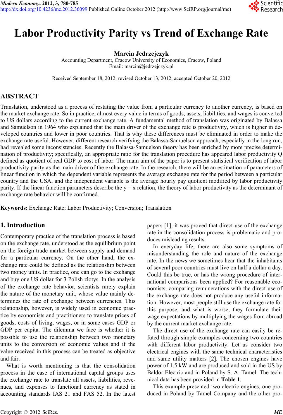
Table 1. Comparative analysis of the 1.5 kW engines manu-
factured in Poland and the USA.
TAMEL (Poland) BALDOR ELECTRIC (USA)
Power 1.5 kW
Sg 90 L-4
B3
400 V
50 Hz
Insulation class F
1200 rpm
Power 1.5 kW
4 Pole
B3 Mounting
460 V
50 Hz
Insulation class F
1140 rpm
SALE PRICE:
424.00 zł $ 637
AFTER TRANSLATION (CONVERSION):
$193 1399.2 zł
duced in the USA by Baldor Electric Co. The end cus-
tomer use of the above-mentioned engines may be con-
sidered the same in spite of the slight differences in pa-
rameters. Table 1 presents the technical specifications of
the engines and selling prices on the domestic markets.
The exchange rate was assumed at the market level of
3.3 zloty per one dollar, according to the conducted
market observation1. If we try to compute the value of
the engine in Polish zloty, we will discover a huge dif-
ference in the resulting amounts. The American price for
the product and the exchange rate between the US dollar
and the Polish zloty gives us a total of 1399.2 zł. There-
fore, preliminary analysis shows great inconsistencies
with the law of one price, which states that the price of
the same or almost the same goods in the different mar-
kets should be equal. We might add that the law of one
price is applied in every methodology specifying conver-
sion rules, but is not necessarily a written law. Using the
exchange rate, which fluctuates but still remains on a
similar level, we can say that the law of one price does
not work in this case at all. This means that the values on
the international scale are incomparable. This was con-
firmed as well by Pakko and Pollard in 1996 on the
BigMac example [3].
It should also be stressed that the US Financial Ac-
counting Standards Board believes that “for an enterprise
operating in multiple currency environments, a true sin-
gle unit of measure does not, as a factual matter, exist”
[4]. In the passage that follows, we read, “the temporal
method obscures the fact of multiple units by requiring
all transactions to be measured as if the transactions oc-
curred in dollars.” The above mentioned method seems
to be treated as the best of all known algorithms. “The
most relevant information about the performance and
financial position of foreign entities is provided by the
functional currency financial statements of those entities.
Using the current exchange rate to restate those func-
tional currency financial statements in terms of their cur-
rent dollar equivalent preserves that most relevant infor-
mation” [4]. These quotes lead one to conclude that the
one and only method of translation in the consolidated
financial statements is based on the exchange rate.
In many published papers, for example W. Kołodko
and others, there is a noticeable tendency to avoid the
exchange rate in international comparisons [5]. Instead of
using the exchange rate, the authors use the so-called
Purchasing Power Standard (PPS), which represents the
equal bundle of goods and services in each country that
underlies the comparison. So, according to the above-
mentioned methodology, GDP is shown in one artificial
currency, which constitutes an attempt to avoid including
the exchange rate in the comparison.
However, there are many aspects of the translation
process, in which noticeable inconsistencies take place.
Therefore, the most important matter is to clarify the
essence of the money and monetary unit value and their
determinants in the international context. In the forth-
coming sections of the paper, labor productivity as the
determinant of the monetary unit value will be formally
presented.
2. Labor Productivity as a Determinant of
Money Value in the International Context
There are many theories describing the exchange rate
behavior. The fundamental assumption is Law of One
Price, formulated by English economist Keith Pilbeam,
stating that equal goods should have the same price on
different markets in the absence of transport costs and
barriers to trade [6]. So-called absolute Purchasing Po-
wer Parity (PPP) is based directly on the Law of One
Price and estimates the exchange rate as the value rela-
tionship between two identical goods on different mar-
kets. For instance, if the bundle of goods costs 200 zł in
Poland and $100 in the US, the exchange rate as defined
as zlotys per dollar should be 200 zł/$100 = 2 zł/$. Thus
the absolute version can be described with the following
simple formula:
P
A
q
ER q ,
where ER = exchange rate, qP = value on the Polish
market, and qA = value on the American market.
The relative PPP argues that the exchange rate adjusts
for inflation differences between two countries:
%∆S = %∆P – %∆P*,
where %∆S = percentage change of the exchange rate,
%∆P = domestic inflation rate, and %∆P* = the foreign
exchange rate. The long-run testing of the relative PPP
had shown many inconsistencies and finally has not been
1The exchange rate has oscillated around 3.3 zloty per one dollar in the
first half of 2012.

M. JEDRZEJCZYK 782
confirmed. For instance, K. Kasa (1995) came to the con-
clusion that PPP explains the dollar-mark exchange rate
trend at 60% but dollar-yen at 20% only [7].
Productivity and its relationship with the exchange rate
were first described in the famous Balassa-Samuelson
research in 1964 [8,9]. The authors argued that direct use
of the exchange rate to convert values in inapplicable.
They drew much attention to productivity differences
between developed countries and poor countries. The au-
thors stated that rich countries have higher productivity
than poor countries, which is why simply multiplying the
foreign prices by the market exchange rate is wrong. To
prove this point, they separated traded goods from un-
traded goods. As Balassa and Samuelson claim, prices of
similar baskets of both traded and untraded goods are
translated into chosen currency, and then the aggregate
price indices will be higher in rich countries than in poor
ones. So it is possible to buy more for one dollar in Po-
land than in the US. Balassa and Samuelson’s research
positively proved the role of productivity in international
comparisons, but had not defined productivity and its
sources. Yet in 1990, M. Dobija [10] has enriched the
Balassa-Samuelson research and stated that this repre-
sents not just productivity, but also labor productivity
differences.
The new approach to the production function, which is
not econometric, but natural, explains the determinants of
wage productivity Q:






QexpAF HexpAFpLexp TF
where A = end-of-period value of assets, H = human
capital, L = constant basic pay (L = p × H), p = the
constant of potential growth (0.08), T = technical equip-
ment of work, and F = level of management. The re-
lationship comes from the transformation of production
function P, since Q is a quotient of production P and cost
of labor W [11]:
AMp
L
PWe
where W = cost of labor, A = assets, L = remuneration
level, and p = economic constant of the potential growth.
In terms of a macroeconomic approach, labor produc-
tivity signed by coefficient Q means the quotient of GDP,
which represents the outcome of global production and
costs of labor (W). The simplest formula for labor pro-
ductivity has been provided below [12]:
GDP
QW 
CCC
GDPW Q
,
where Q = labor productivity and W = cost of labor.
In order to formally present the method of estimating
labor productivity ratio Q using observed values of the
market exchange rate and to present relationships be-
tween coefficients, we take the real GDP, which repre-
sents the nominal GDP expressed in the last years’ prices
for a chosen country and the USA. We consider the GDP
to be a product of wage (cost of labor) W and real pro-
ductivity coefficient (Q). The subscript C denotes a given
country, and subscript A is the American wage and real
productivity. Thus the equations can be written as fol-
lows:


AAA
GDPW Q


After dividing the above equations:
CCC
AAA
GDPW Q
GDPW Q


.
Then reformulating following formula can be obtain-
ed:

CC
CA
AA
WQ
GDP złGDP $
WQ
.
The above formula shows some applications of the
exchange rate. Therefore, we write a subsequent formula,
where f(ER) denotes some function of the exchange rate.




CA
GDP złf(ER) GDP$

Dividing labor cost W by number of employees, we
obtain a formula in which (AP) represents average pay
and E is the number of employees of the given countries:

CC C
CA
AA A
AP EQ
GDP złGDP $
AP EQ


.
Dividing GDP by number of employees E, we get the
equation:

CC
CA
AA
AP Q
GDPE złGDPE $
AP Q
 ,
where GDPE = GDP per one employee. So the funda-
mental relationship is:
CA
AC
WQ
WQ




,
and it can be treated as an equalizing mechanism for
countries with different productivity.
For instance, the value of coefficient Q for Poland in
2010 accounted for 1.9 and for USA 3.45. This means
that, in Poland, 1 zloty of labor cost generated 1.9 GDP,
and in the US, 1 dollar generated 3.45 dollars of GDP.
This shows a noticeable difference in productivity be-
tween the two countries. That is why, by comparing
minimum wages in Poland (10 zlotys per hour) and in the
USA ($7.25 per hour), it is impossible to estimate the
real exchange rate, which is now about 3.3 zlotys per one
dollar. On the other hand, direct use of the exchange rate
for translating American minimum wage to Polish zloty

M. JEDRZEJCZYK 783
will bring 25 zlotys per hour, which is highly improbable
in Poland. This happens because the direct use of the
exchange rate is inapplicable to the conversion of wages
because of the previously mentioned differences in wage
productivity. Table 2 shows the rates of the Q factor for
several countries, starting from the year 2006 and ending
in 2011.
Now it is clear that the direct use of the exchange rate
is theoretically possible only in the case of countries with
similar Q factors; for instance, the USA, the UK, Japan,
and Germany. In other presented cases, the direct use of
the exchange rate to convert values between countries
will fail and bring the wrong results. However, knowing
the value of Q coefficient, it is possible to modify the
equation that assumes the equality of the considered
economic systems:
CA
AC
QER
WQ

W
where Wc = average pay in particular country, WA =
American average pay, Qc = wage productivity of par-
ticular country, QA = American wage productivity, and
ER = average exchange rate.
The above equation constitutes the basics for statistical
verification of the linear model designed in the forth-
coming part of the paper.
3. Market Exchange Rate and Labor
Productivity—The Model
Research comparing the market exchange rate trend and
the exchange rate estimated with the relationship of
hourly cost of labor modified by the quotient of labor
productivity factor Q between the USA and the selected
country needs to be based on a set of countries with the
available market floating exchange rates to the US dollar.
The US dollar has been chosen as the base currency in
the research, as all international comparisons are made
after translation to the US dollar, and the American eco-
nomic system has been always treated as a base for other
countries. What is more important is that the sample
Table 2. Value of Q factor for chosen countries in years
2006-2011.
2006 2007 2008 2009 2010 2011
Poland 1.881 1.992 1.854 1.869 1.903 1.935
Switzerland 3.534 3.645 3.748 3.65 3.509 3.498
UK 3.204 3.517 3.444 3.082 3.095 3.216
USA 3.458 3.47 3.56 3.5 3.4523.648
Japan 3.069 3.093 3.186 3.433 3.279 3.448
Germany 3.305 3.38 3.389 3.276 3.169 3.158
must consist of countries with different labor productive-
ity to prove the main thesis.
The needed data to conduct the statistical analysis has
been collected from official statistical sources of consid-
ered countries. The average hourly wage estimates of
selected countries have been provided in Table 3.
Since, as mentioned above, the direct use of the ex-
change rate in the case of countries with different pro-
ductivity is inapplicable, two data streams have been
chosen for linear regression. The first data stream is the
trend of the exchange rate between selected countries,
and the second stream is the trend of labor cost relation-
ship. The function form for estimating parameters a and
b has been provided below. The results confirming the
tested theory would be the best if parameter a were close
to 1 and parameter b were close to 0.
CA
AC
WQ
ER ab
WQ





The forthcoming tables are calculations of the rela-
tionship


cA
WW (Table 4),

QQ
AC
(Table 5) and




WWQQ
CA AC
(Table 6) that lead finally to the
estimation of a and b parameters of linear function. The
most expected result is a close to 1 and b close to 0.
Table 7 shows average market exchange rates for
years 2006-2010 to the US dollar collected. The data
come from the OANDA exchange rate website [13].
The chosen linear regression method is based on the
ordinary least squares estimation (OLS), since the me-
thod is quite simple and easy to interpret. The results
Table 3. Estimated average hourly pay in years 2005 to
2010 (estimates for 2011 are still unavailable).
Country 2005 2006 2007 2008 2009 2010
Poland [zł] 23.220 24.420 27.000 28.000 31.000 33.000
UK [£] 9.4909.84010.140 10.540 10.990 11.090
USA [$] 16.120 16.750 17.430 18.080 18.620 19.075
Japan [¥] 2028 2078 2112 1990 1975 2083
Germany [€]16.716.55 17.61 18.11 18 17
Table 4. Estimated quotient between hourly pay in a par-
ticular country to the US hourly pay from 2006 to 2010.
Country 2006 2007 2008 2009 2010
Poland [zł/$] 1.457911.54905 1.54867 1.664871.73001
UK [£/$] 0.587460.58175 0.58296 0.590220.58138
USA 1 1 1 1 1
Japan [¥/$] 124.059 121.170 110.0664 106.0687 109.2005
Germany [€/$]1.03598 0.98806 1.010327 1.001659 0.966702

M. JEDRZEJCZYK 784
Table 5. Estimated quotient between labor productivity Q
in the US to the particular country between years 2006 to
2010.
Country 2006 2007 2008 2009 2010
Poland 1.838384 1.741968 1.920173 1.872659 1.813978
UK 1.079276 0.986636 1.033682 1.135626 1.115347
USA 1 1 1 1 1
Japan 1.126751 1.121888 1.117389 1.019516 1.05276
Germany 1.046293 1.026627 1.050457 1.068376 1.089303
Table 6. Estimated product of quotient between hourly pay
in particular country to US hourly pay and the quotient
between labor productivity Q in the US to the particular
country during years 2006 to 2010.
Country 2006 2007 2008 2009 2010
Poland [zł/$] 2.68019 2.698402.97371 3.11774 3.13820
UK [£/$] 0.6340 0.573980.6026 0.6702760.648451
USA 1 1 1 1 1
Japan [¥/$] 139.78 135.936 122.986 108.138 114.961
Germany [€/$] 1.0839 1.014361.061305 1.0701491.053032
Table 7. Average exchange rates to the US dollar during
years 2006 to 2010.
Country 2006 2007 2008 2009 2010
Poland [zł/$] 3.10357 2.765612.40784 3.117573.01639
UK [£/$] 0.54346 0.499800.54481 0.641030.64742
USA 1 1 1 1 1
Japan [¥/$] 116.315 117.792103.442 93.596187.8064
Germany [€/$] 0.796905 0.730715 0.68331 0.719055 0.75476
of the linear function parameters estimation have been
provided below.
a = 0.8348, b = 0.0795
thus, the estimated functional relationship between the
exchange rate and proposed equation

CA A
Q

C
WWQ can be formulated as follows:
C
W
ER0.8348 WQ 
A
AC
Q0.0795




Table 8 presents the results for all tested time periods,
starting from the year 2006 and ending at 2010. In every
case, the parameter a value is close to one and b is close
to 0.
The parameter a according to the OLS method equals
0.8348 and b is 0.0795 for all data sets gathered during
the research, which is very close to the expected results.
As parameter a is close to 1 and b is close to 0, we can
formulate the general motion:
CA
AC
WQ
ER WQ




Table 9 presents the parameters of stochastic structure,
which also confirms accurate adjustment of variables to
the gathered empirical data.
The model describes well the tested dependence be-
tween the average exchange rate (ER) and the proposed
indicator




WWQ Q
CA AC
. Variance S2 equals
5.4687, and the standard deviation S: 2.33 and deter-
mination ratio (φ2) are very close to zero and equal 0.25%,
which is more than satisfactory. However, the variation
coefficient (V) is a bit higher, because the dependent
value is distorted by the exchange rate of Yen to US dollar
(more than 100), which is much higher than other rates
belonging to the range of 0.5 to 3.
4. Conclusion
For the empirical assessment of the labor productivity
bias hypothesis, certain countries with different labor
productivity (Q) value have been chosen. The model is
an example of the linear regression function, which has
confirmed the usefulness of the labor productivity (Q)
factor in estimating the exchange rate as the quotient of
average hourly pay. Empirical results, especially the sto-
chastic structure parameters, suggest that labor pro-
ductivity bias hypothesis holds for all countries during
the entire period considered. The linear model proves that
the relationship between the average exchange rate and
the formula




WWQ Q
CA AC
can be described as a
y = x function, which sacrifices the tested hypothesis and
fully enables the possibility of using the formula in the
Table 8. Estimation of a and b parameters for the years
2006 to 2010.
Parameter
estimates 20062007 2008 2009 2010 Overall 2006-2010
a 0.8630.7610.8419 0.865 0.831 0.8348
b 0.2120.247−0.098 0.097 0.1278 0.0795
Table 9. Stochastic structure of the linear regression model
based on chosen OLS method.
Parameters2006 2007 2008 2009 2010 Overall
2006-2010
S2 0.5010.1630.012 0.98 0.067 5.4687
S 0.2510.40450.11 0.3131 0.259 2.3385
φ2 0.01%0.01%0% 0% 0% 0.25%
V 2.05% 1.76% 0.41% 1.02% 0.86% 8.66%

M. JEDRZEJCZYK 785
international comparisons. It is worth emphasizing that
the hypothesis holds firm in the case of countries with
different Q factors and similar Q factors, what can be
treated as a full confirmation of the labor productivity
parity approach. The research also confirms Balassa-
Samuelson research in a way, because the value of labor
productivity indicator (Q) is higher for rich countries and
lower for developing countries. However, even more
important is that this procedure will enable one to con-
duct truthful and fair translation processes and will show
the adequate value in international comparisons for
wages and prices. So far, GDP or GDP per Capita has
been used to measure economic development and the
welfare of societies, and surely it can be replaced by
productivity coefficient Q. What is more, Q is unrated
value and is very easy to interpret.
REFERENCES
[1] M. Jedrzejczyk, “Value Translation in Consolidated Fi-
nancial Statements of the International Capital Groups,”
Polskie Towarzystwo Ekonomiczne, Cracow, 2009.
[2] M. Jedrzejczyk, “Towards the Best Procedure of Transla-
tion,” In: I. Górowski, Ed., General Accounting Theory,
Evolution and Design for Efficiency, Wydawnictwa Aka-
demickie i Profesjonalne, Warsaw, 2008.
[3] M. Pakko and P. Pollard, “For Here or To Go? Purchas-
ing Power Parity and the Big Mac,” Review of the Fed-
eral Reserve Bank of Saint Louis, Vol. 78, No. 1, 1996,
pp. 3-21.
[4] Financial Accounting Standards Board, “Original Pro-
nouncements 1998/1999 Edition,” John Wiley and Sons,
Hoboken, 1998.
[5] W. G. Kołodko, “About Fixing Our Finance,” TNOiK,
Toruń, 2004.
[6] K. Pilbeam, “International Finance,” 3rd Edition, Mac-
Millan Business, London, 2006
[7] K. Kasa, “Understanding Trends in Foreign Exchange
Rates,” FRBSF Weekly Letter, Vol. 95, No. 22, 1995.
[8] B. Balassa, “The Purchasing Power Party Doctrine: A
Reappraisal,” Journal of Political Economy, Vol. 72, No.
6, 1964, pp. 584-596.
[9] P. Samuelson, “Theoretical Notes on Trade Problems,”
Review of Economics and Statistics, Vol. 46, No. 2, 1964,
pp. 145-154.
[10] M. Dobija, “Labor Productivity vs Minimum Wage Le-
vel,” Modern Economy, Vol. 2, No. 5, 2011, pp. 780-787.
doi:10.4236 /me.2011.25086
[11] M. Dobija, “Abstract Nature of Money and the Modern
Equation of Exchange,” Modern Economy, Vol. 2, No. 2,
2011, pp. 142-152. doi:10.4236/me.2011.22019
[12] M. Dobija and M. Jędrzejczyk, “Conversion of Values to
One Money Unit in Consolidation Process,” Emergo:
Journal of Transforming Economies and Societies, Vol.
11, No. 4, 2004.
[13] http://www.oanda.com