Discretionary Fiscal Policy and the European Monetary Union

doi:10.4236/me.2012.36095

Paper Menu >>

Journal Menu >>

Modern Economy, 2012, 3, 742-751

http://dx.doi.org/10.4236/me.2012.36095 Published Online October 2012 (http://www.SciRP.org/journal/me)

Discretionary Fiscal Policy and the European

Monetary Union

Jason Jones

Department of Economics, Furman University, Greenville, USA

Email: jason.jones@furman.edu

Received August 10, 2012; revised September 17, 2012; accepted September 26, 2012

ABSTRACT

A model of circumstances that can lead to changes in the way a fiscal authority conducts policy after joining a monetary

union is presented and empirically tested for the euro area. According to the model consolidation fatigue, shock asym-

metry, or differences in the relative weight placed on output/price stabilization between the new and old monetary au-

thority can lead to greater reliance on fiscal policy. Empirical evidence suggests that there has been a change in the

conduct of fiscal policy in the euro area which is most likely due to consolidation fatigue and a stronger emphasis on

price stabilization by the European Central Bank.

Keywords: Fiscal Policy; Policy Interaction; EMU

1. Introduction

The sovereign debt crisis among members of the Euro-

pean Monetary Union (EMU) underscores the need to

study fiscal policy in the currency union. In the years

immediately preceding the formation of the monetary

union the budgetary position of most members improved.

Soon after the formation of the monetary union, however,

budgetary positions began to deteriorate. The deteriora-

tion of fiscal positions in relatively good times made the

deficit effects of the global recession in the late 2000s

severe, leading to debt crises and bailouts of some of the

member states.

The change in fiscal balances soon after the creation of

the EMU suggests that part of the explanation could be

tied to the monetary union itself. Understanding how the

monetary union has modified the role and preferences of

its policymakers can help the union address its deficit

challenges. This understanding can also inform states

looking to join the EMU, as well as other monetary un-

ions under consideration around the world, of the possi-

ble fiscal challenges they may face.

This paper models and tests possible changes to dis-

cretionary fiscal policy as a result of becoming a member

of the EMU. By expanding Uhlig’s [1] model of policy

interaction and applying it both before and after the for-

mation of the monetary union, the fiscal challenges of

surrendering independent monetary policy are illustrated.

Specifically, increased reliance on ﬁscal management is

needed if shocks are dissimilar across members of the

monetary union or the policy weights of the new mone-

tary authority are different than the former local mone-

tary authority. The model also allows for an exogenous

change in the preferences of fiscal authorities to account

for consolidation fatigue identified by Hughes-Hallett

and Lewis [2].

To test this model and understand how discretionary

fiscal policy has changed in the euro area, a fiscal reac-

tion function is estimated allowing for a break at the

formation of the monetary union in 1999. Unlike most

fiscal reaction function literature, the response to supply

and demand shocks rather than the output gap is esti-

mated. The results suggest that there has been a change

in the way fiscal authorities respond to supply shocks

since becoming members of the EMU. The response be-

comes counter-cyclical after the formation of the union

and is most likely due to a stronger weight by the Euro-

pean Central Bank (ECB) on price stabilization relative

to output stabilization compared to the former local

monetary authority. Counter-cyclical fiscal responses

after the formation of the union could help explain the

worsening of budgetary balances. In addition, the fiscal

response to debt levels is weaker after the formation of

the EMU. This result suggests a role for consolidation fa-

tigue in explaining worsening deficit positions.

The remainder of the paper is structured as follows. In

the next section a model of monetary and ﬁscal policy is

constructed that explores the possible reasons for chan-

ges in the conduct of discretionary fiscal policy as a re-

sult of joining a monetary union. The following two sec-

tions introduce the empirical techniques and data used to

test how fiscal reactions have changed since the forma-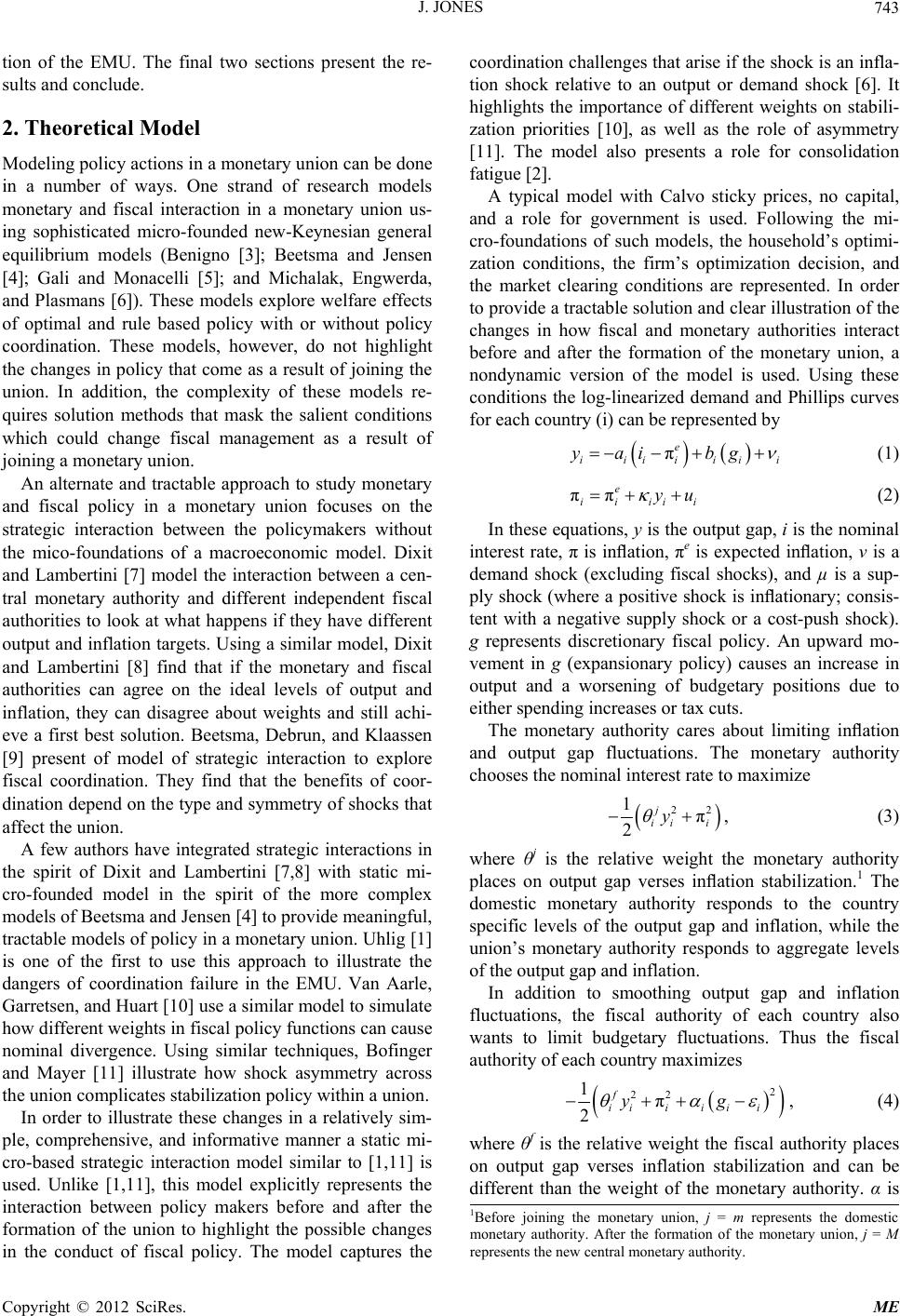

J. JONES 743

tion of the EMU. The final two sections present the re-

sults and conclude.

2. Theoretical Model

Modeling policy actions in a monetary union can be done

in a number of ways. One strand of research models

monetary and fiscal interaction in a monetary union us-

ing sophisticated micro-founded new-Keynesian general

equilibrium models (Benigno [3]; Beetsma and Jensen

[4]; Gali and Monacelli [5]; and Michalak, Engwerda,

and Plasmans [6]). These models explore welfare effects

of optimal and rule based policy with or without policy

coordination. These models, however, do not highlight

the changes in policy that come as a result of joining the

union. In addition, the complexity of these models re-

quires solution methods that mask the salient conditions

which could change fiscal management as a result of

joining a monetary union.

An alternate and tractable approach to study monetary

and fiscal policy in a monetary union focuses on the

strategic interaction between the policymakers without

the mico-foundations of a macroeconomic model. Dixit

and Lambertini [7] model the interaction between a cen-

tral monetary authority and different independent fiscal

authorities to look at what happens if they have different

output and inflation targets. Using a similar model, Dixit

and Lambertini [8] find that if the monetary and fiscal

authorities can agree on the ideal levels of output and

inflation, they can disagree about weights and still achi-

eve a first best solution. Beetsma, Debrun, and Klaassen

[9] present of model of strategic interaction to explore

fiscal coordination. They find that the benefits of coor-

dination depend on the type and symmetry of shocks that

affect the union.

A few authors have integrated strategic interactions in

the spirit of Dixit and Lambertini [7,8] with static mi-

cro-founded model in the spirit of the more complex

models of Beetsma and Jensen [4] to provide meaningful,

tractable models of policy in a monetary union. Uhlig [1]

is one of the first to use this approach to illustrate the

dangers of coordination failure in the EMU. Van Aarle,

Garretsen, and Huart [10] use a similar model to simulate

how different weights in fiscal policy functions can cause

nominal divergence. Using similar techniques, Bofinger

and Mayer [11] illustrate how shock asymmetry across

the union complicates stabilization policy within a union.

In order to illustrate these changes in a relatively sim-

ple, comprehensive, and informative manner a static mi-

cro-based strategic interaction model similar to [1,11] is

used. Unlike [1,11], this model explicitly represents the

interaction between policy makers before and after the

formation of the union to highlight the possible changes

in the conduct of fiscal policy. The model captures the

coordination challenges that arise if the shock is an infla-

tion shock relative to an output or demand shock [6]. It

highlights the importance of different weights on stabili-

zation priorities [10], as well as the role of asymmetry

[11]. The model also presents a role for consolidation

fatigue [2].

A typical model with Calvo sticky prices, no capital,

and a role for government is used. Following the mi-

cro-foundations of such models, the household’s optimi-

zation conditions, the firm’s optimization decision, and

the market clearing conditions are represented. In order

to provide a tractable solution and clear illustration of the

changes in how ﬁscal and monetary authorities interact

before and after the formation of the monetary union, a

nondynamic version of the model is used. Using these

conditions the log-linearized demand and Phillips curves

for each country (i) can be represented by







πe

iiiiiii

yai bg







ππ

iiiii

(1)







(2)

In these equations, y is the output gap, i is the nominal

interest rate, π is inﬂation, πe is expected inﬂation, ν is a

demand shock (excluding fiscal shocks), and µ is a sup-

ply shock (where a positive shock is inﬂationary; consis-

tent with a negative supply shock or a cost-push shock).

g represents discretionary fiscal policy. An upward mo-

vement in g (expansionary policy) causes an increase in

output and a worsening of budgetary positions due to

either spending increases or tax cuts.

The monetary authority cares about limiting inﬂation

and output gap fluctuations. The monetary authority

chooses the nominal interest rate to maximize



1π

ii i





, (3)

where θj is the relative weight the monetary authority

places on output gap verses inﬂation stabilization.1 The

domestic monetary authority responds to the country

specific levels of the output gap and inflation, while the

union’s monetary authority responds to aggregate levels

of the output gap and inflation.

In addition to smoothing output gap and inflation

fluctuations, the fiscal authority of each country also

wants to limit budgetary fluctuations. Thus the fiscal

authority of each country maximizes







1π

iiii ii



, (4)

where θf is the relative weight the fiscal authority places

on output gap verses inflation stabilization and can be

different than the weight of the monetary authority. α is

1Before joining the monetary union, j = m represents the domestic

monetary authority. After the formation of the monetary union, j =

represents the new central monetary authority.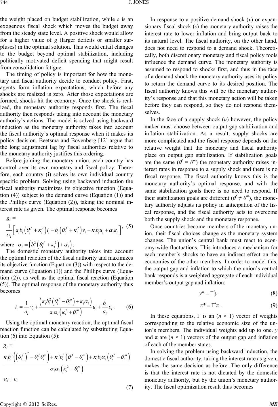

J. JONES

744

the weight placed on budget stabilization, while ε is an

exogenous fiscal shock which moves the budget away

from the steady state level. A positive shock would allow

for a higher value of g (larger deficits or smaller sur-

pluses) in the optimal solution. This would entail changes

to the budget beyond optimal stabilization, including

politically motivated deficit spending that might result

from consolidation fatigue.

The timing of policy is important for how the mone-

tary and ﬁscal authority decide to conduct policy. First,

agents form inﬂation expectations, which before any

shocks are realized is zero. After those expectations are

formed, shocks hit the economy. Once the shock is real-

ized, the monetary authority responds first. The ﬁscal

authority then responds taking into account the monetary

authority’s actions. The model is solved using backward

induction as the monetary authority takes into account

the ﬁscal authority’s optimal response when it makes its

policy decision. Beetsma and Bovenberg [12] argue that

the long adjustment lag by fiscal authorities relative to

the monetary authority justifies this ordering.

Before joining the monetary union, each country has

control over its own monetary and ﬁscal policy. There-

fore, each country (i) solves its own individual country

specific problem. Solving using backward induction the

ﬁscal authority maximizes its objective function (Equa-

tion (4)) subject to the demand curve (Equation (1)) and

the Phillips curve (Equation (2)), taking the nominal in-

terest rate as given. The optimal response becomes



iiiiiiiii

abi bviiiii











 













22f

, (5)

where iiii i



 

.

The domestic monetary authority takes into account

the optimal reaction of the ﬁscal authority and maximizes

its objective function (Equation (3)) with respect to the de-

mand curve (Equation (1)) and the Phillips curve (Equa-

tion (2)), as well as the optimal ﬁscal reaction (Equation

(5)). The optimal response of the monetary authority thus

becomes



1fm

ii ii

ii m

ii ii

iv a



i ii





 



 



. (6)

Using the optimal monetary reaction, the optimal ﬁscal

reaction function can be calculated by substituting Equa-

tion (6) into Equation (5):



333

ffm fm

iiiiii iiiii

ii ii

 

 





 





In response to a positive demand shock (ν) or expan-

sionary fiscal shock (ε) the monetary authority raises the

interest rate to lower inflation and bring output back to

its natural level. The ﬁscal authority, on the other hand,

does not need to respond to a demand shock. Theoreti-

cally, both discretionary monetary and fiscal policy tools

influence the demand curve. The monetary authority is

assumed to respond to shocks first, and thus in the face

of a demand shock the monetary authority uses its policy

to return the demand curve to its desired position. The

fiscal authority knows this will be the monetary author-

ity’s response and that this monetary action will be taken

before they can respond, so they do not respond them-

selves.

In the face of a supply shock (u) however, the policy

maker must choose between output gap stabilization and

inflation stabilization. As a result, supply shocks are

more complicated and the fiscal response depends on the

relative weight that the monetary and ﬁscal authority

place on output gap stabilization. If stabilization goals

are the same (θf = θm) the monetary authority raises in-

terest rates in response to a supply shock and there is no

fiscal response. The fiscal authority knows this is the

monetary authority’s optimal response, and with the

same stabilization goals there is no need to respond. If

their stabilization goals are different (θf ≠ θm), the mone-

tary authority adjusts its policy in anticipation of the fis-

cal response, and the fiscal authority acts to overcome

both the supply shock and the monetary response.

Once countries become members of the monetary un-

ion, their ﬁscal choices change as the monetary system

changes. The union’s central bank must react to econ-

omy-wide fluctuations. This introduces a mechanism for

each member’s shocks to have an indirect effect on the

economies of the other members. In order to model this,

the output gap and inﬂation to which the union’s central

bank responds is a weighted aggregate of each individual

member’s output gap and inﬂation:

i ii





*yy



(7)





π*π



(8)

. (9)





In these equations, Γ is an (

n × 1) vector of weights

corresponding to the relative economic size of the un-

ion’s members. The individual weights add up to one. y

and π are (n × 1) vectors of the output gap and inﬂation

of each of the member states.

In solving the problem using backward induction, the

domestic ﬁscal authority, taking the interest rate as given,

makes the same decision as before. The only difference

is that the interest rate is not dictated by the domestic

monetary authority, but by the union’s monetary author-

ity. The ﬁscal optimization result thus becomes

J. JONES 745



gab ibii

vbu



















.(10)

In this case, i* is the nominal interest rate dictated by

the union’s monetary authority. The subscript (i) on the

parameters has been dropped because it has been as-

sumed for clarity and illustrative purposes that each

country has the same parameters across the union.

The union’s monetary authority now takes into ac-

count the aggregate output gap and inﬂation of the mem-

ber states, as well as the aggregate ﬁscal reaction, and

maximizes





*π

y



. (11)

The optimal monetary policy for the union’s monetary

authority thus becomes



 





 





 

. (12)

In this case, ν, µ, and ε are (n × 1) vectors of country

specific shocks. This reaction is similar to the domestic

monetary authority’s actions except the new monetary

authority reacts to weighted averages of the country spe-

cific shocks. In order to solve for the domestic optimal

fiscal policy once the union’s monetary authority has

acted, it is convenient to rewrite Equation (12) as



iim

 

 

 

ii ii















 





 





 

. (13)

Here,  is the vector of weights i



11n ()



excluding the weight of country (i). Similarly ν, µ, ε are

the vectors of shocks excluding country (i).

Plugging Equation (13) into Equation (10) gives the fol-

lowing optimal fiscal response:



11n







 

 



 





 

















22 22

()

fM f

 



  





 

 



 





















 







 



, (14)

where If

shocks and weights are identical across the monetary

union, this expression is the same as the one country

case.2



33ffM

 



A comparison of Equation (7), the ﬁscal authority’s

optimal reaction before the formation of the union, and

Equation (14), the optimal reaction after the formation of

the union, illustrates how the role of the domestic ﬁscal

authority could change after the formation of the mone-

tary union. The ﬁscal authority now must take into ac-

count how large its country is in relation to other mem-

bers as well as how similar country specific shocks are to

those in the rest of the union. They also must take into

account how the new monetary authority’s relative

weight on output stabilization may be different than that

of the previous domestic monetary authority.

Sufficient similarity in shocks and thus synchronized

business cycles was cited by Mundell [13] as a necessary

criterion for a group of countries to be an optimal cur-

rency area (OCA). The problem of not meeting this OCA

criterion for the ﬁscal authority can be seen by compare-

ing Equations (7) and (14). For example, before joining

the union the ﬁscal authority did not need to respond to

any demand shocks, yet after the formation of the union

the ﬁscal authority optimally responds to a demand shock

when the country specific shock is different than that of

the aggregate shock. Assume a member state experiences

a country specific negative demand shock (νi) while the

average demand shock for all members in that period

(







) is positive. The local ﬁscal authority must now

increase deficits (or reduce surpluses) in response to its

negative country specific demand shock:





















 





. (15)

At the same time, they must increase spending to

overcome the monetary authority’s response to the un-

ion-wide positive demand shock:











.

(16)









Before monetary unification, the country specific fis-

cal authority did not need to react to its own demand

shock, nor was it concerned with the symmetry of that

shock (in relation to its neighbors). After joining the un-

ion, shock asymmetry would lead to an increased role for

the local fiscal authority.

Greater reliance on ﬁscal policy may also be necessary

if the monetary union’s central bank has a response func-

tion different than that of the country’s monetary author-

ity. For example, the union’s monetary authority’s pref-

erence for output stabilization could be less than that of

2For example



ii M

 



if all fiscal shocks are the same.

This relationship is true for each shock.

J. JONES

746

the country’s prior monetary authority (θM < θm). This is

a distinct possibility for many countries in euro area with

weak domestic central banks. The ECB adopted the

German model of central banking (with a strong repute-

tion for fighting inflation) and a one pillar strategy of

monetary policy on inflation stabilization (Wyplosz [14]).

In order to maintain the same level of output stabilization

as before, a ﬁscal authority may have to act more aggres-

sively because of the weaker response of the central bank.

To illustrate, assume that the shocks that hit the economy

are the same so the optimal reaction for the ﬁscal author-

ity is illustrated by Equation (7). If the weight the mone-

tary authority placed on output stabilization changes, the

ﬁscal reaction changes as follows:



22 22

bb b



bb u





 



 





 







(17)

where 2



 



01 11txttbtdtt



.

In this case, even if there is a common cost push shock

across the union, the ﬁscal authority increases deficits or

reduces surpluses if the new monetary authority is plac-

ing less weight on output stabilization (θm falls). The case

is similar for demand and ﬁscal shocks if there is shock

asymmetry.

It is also possible that the changes in the deﬁcit are not

structural at all, but that greater deﬁcits are a result of

changes in political will. In an attempt to meet the deﬁcit

criterion of the Maastricht Treaty, most countries had to

implement sometimes painful structural as well as tem-

porary changes to their budgets. For example, in the run

up to the formation of the monetary union Italy went

through major pension reform, raising the retirement age

and increasing individual contributions in an attempt to

cut down the budget deﬁcit. In addition, temporary ad-

justments were made that did not change the structure of

the deﬁcit but did bring it in line with the Maastricht cri-

teria. Italy used the sale of public assets to increase gov-

ernment revenue, delayed contract renegotiations, and

even imposed a temporary Eurotax. Such reforms and

one-off measures are hard to maintain especially when

the promised returns from joining the union have been

slow in coming. Member state populations and politi-

cians may tire from the ﬁscal constraints imposed on

them.

After the formation of the union, the deficit restrictions

in the Maastricht treaty were extended under the Stability

and Growth Pact (SGP). Under the Maastricht criteria,

rule violation would keep a country out of the union.

Punishment for violating the SGP, on the other hand,

comes in the form of fines. These fines are imposed by

fellow members who have little incentive to strap their

already strapped neighbors with further financial obliga-

tions. In such a way, governments have less incentive to

meet the somewhat arbitrary deﬁcit rules, especially

when there are economic strains at home. Eichengreen

and Wyplosz [15] suggest that European governments

traditionally have a deﬁcit bias. If politicians become

tired of reform, run out of temporary measures, and see

the enforcement of the SGP as weak, then worsening

deficits would be expected. Such consolidation fatigue

has been identified by Hughes-Hallett and Lewis [2] as

an important reason for the worsening of deficit positions

after the formation of the monetary union in Europe. In

terms of the model, if all the fiscal authorities decided

(irrespective of output or price fluctuations) to have

higher deficits once they enter the union, fiscal balances

will change in a one to one fashion.

3. Testing the Nature of Responses

In order to test for possible changes in the conduct of

fiscal policy illustrated in the model, a fiscal reaction

function is estimated. A fairly standard approach to

measuring fiscal reaction functions exists in the literature

and consists of estimating versions of the following

model:

EXbf u









. (18)

In this model, current fiscal policy (ft) is a function of

the expected value of a macroeconomic indicator (Et-1 Xt),

last period’s debt level (bt-1), and last period’s fiscal

stance (dt-1). Most studies of fiscal reaction functions use

both the cyclically adjusted primary budget balance to

measure discretionary fiscal policy and the noncyclically

adjusted primary budget balance to study automatic sta-

bilizers. The primary balance is used to remove any in-

fluence changes in the interest paid on existing debt may

have on the budgetary balance. The macroeconomic in-

dicator most often used is the output gap. To estimate the

expected value, most authors use an instrumental vari-

able approach. The debt to GDP ratio is used to capture

any fiscal authority’s motivation to stabilize debt levels.

The lag of the fiscal variable is included to account for

possible autocorrelation in the budget decision.

The estimation of fiscal reaction functions in the EMU

has received a fair amount of attention in the literature.

Most of these explore how deficit restrictions impact the

way fiscal authorities operate in the euro area. Gali and

Perotti [16] find a change in the conduct of discretionary

fiscal policy since the budgetary restrictions were intro-

duced in the Maastricht Treaty. Whereas discretionary

fiscal policy was procyclical before Maastricht they have

become more counter-cyclical since that time (specifi-

J. JONES 747

cally they have become less procyclical). This result in-

dicates that the deficit restrictions have not prevented the

fiscal authorities from exercising discretionary fiscal

policy as was feared.

Wyplosz [14] finds support for [16] conclusions using

the same empirical strategy on updated data. Garciá, Ar-

royo, Minguez, and Uxó [17] estimate the fiscal rule for

each country in the euro area using seeming unrelated

regression and find that policy was most procyclical

pre-Maastricht, and though it was still procyclical post-

Maastricht it was not nearly as strong and for many

countries it became acyclical. Von Hagen [18], on the

other hand, using pooled data instead of panel data finds

that discretionary policy has remained strongly procycli-

cal since Maastricht. Balassone, Francese, and Zotteri

[19] find no change in the way fiscal policy is conducted

since the introduction of fiscal restrictions, but they do

find cyclical asymmetry; discretionary policy is counter-

cyclical when there is a negative output gap, but does not

respond at all to positive output gaps. Using more current

data, Candelon, Maysken, and Vermeulen [20] find that

contrary to [16], discretionary policy has remained

strongly procyclical since Maastricht.

Due to data restrictions and the emphasis on the deficit

restrictions, which change little after the actual formation

of the union, only [17] test for changes in fiscal reactions

after the formation of the union. They find little change

in the way fiscal authorities respond to the output gap

when compared to the Maastricht period. These results,

however, do not reflect the possible changes to policy

that can come as a result of joining the union because

they do not identify what types of shocks lead to changes

in the output gap. As the model introduced in the previ-

ous section predicts, the type of shock is important when

looking at fiscal reaction functions before and after join-

ing a monetary union.

Candelon et al. [20] attempt to account for the sources

of output gap fluctuations. They use the European Com-

mission’s Business and Consumer Survey. Question

eight of the Industry/Business Climate Indicator, asks

companies about the most important factor limiting their

production. Answers of demand or financial constraints

are categorized as demand shocks, while responses of

labor or equipment were categorized as supply shocks.

These responses are aggregated to the country level to

create a supply and demand variable for each country in

each time period. They find that deficits increase when

there are supply constraints on firms, but they decrease

when there are demand constraints. This strategy of iden-

tifying supply and demand shocks has limitations in

terms of our model. Labor or equipment limitations on

firm production could be the result of either a supply or a

demand shock to the economy as a whole.

Strawczynski and Zeira [21] estimate fiscal reaction

functions for twenty-two OECD countries using perma-

nent and transitory shocks in the place of the output gap.

To identify these shocks they use the Blanchard and

Quah [22] technique of long run-restrictions on a VAR.

The use of long-run restrictions in VARs has been used

by a number of authors to identify supply and demand

shocks in Europe (Bayoumi and Eichengreen [23]; Fidr-

muc and Korhonen [24]; and Babetski, Boone, and

Maurel [25]). In order to identify structural shocks from

a reduced form VAR, certain restrictions, derived from

economic theory, must be introduced. Long-run restric-

tions rely on theoretical differences in how variables re-

spond to shocks at different time horizons. The restric-

tions used to identify supply and demand shocks are

based on assumptions derived from simple Keynesian

predictions. Theory suggests that while demand shocks

influence prices in the long run, they have no long-run

effect on output. Supply shocks, on the other hand, do

have permanent effects on both output and prices. The

restriction of no demand effects on output in the long run

allows for identification using the Blanchard and Quah

technique.

These identified shocks more closely match the shocks

from the theoretical model presented in the previous sec-

tions and are used in the place of the output gap. As a

result, the following panel response function is estimated

to test the theoretical model and potential changes in fis-

cal policy:

BE AEBEAE

,01, 2, 3, 4,

BE AE

5,1 6,1 7,1,

itit ititit

ititit it

ssdd

bb f

 

 

 

 

  . (19)

Here, f and b are respectively the fiscal stance and debt

level. Supply shocks (s) and demand shocks (d) replace

the output gap in Equation (18). Supply shocks, demand

shocks, and the debt are split to before (BE) and after

(AE) the formation of the EMU. In this way a simple

Wald test can be used to determine if there is a difference

in the way the fiscal authority reacts to these variables

after the formation of the union. The expected value of

the supply and demand shocks is not needed as, by defi-

nition, they should be surprises. The current value of the

supply and demand shocks is used because the data are

annual. At this frequency the authorities’ have enough

time to respond to shocks within the period.3

A panel fixed effects estimator as well as the Arellano

and Bond [26] two-stage GMM estimator are used to

estimate the fiscal reaction function. The Arellano and

Bond estimator is used to account for possible correlation

between the lagged dependent variable and the unob-

served panel-level effects, which would make the fixed

effects estimator in a dynamic panel model inconsistent.

3Robustness tests have been run which use the lag of supply and de-

mand shocks with very similar results.

J. JONES

748

Robust standard errors are estimated to correct for possi-

ble heteroskedasticity.

4. Data

The data come from AMECO, the European Commission

Economic and Financial Affairs annual macro-economic

database and are recorded from 1978 to 2010. Eleven of

the original twelve members of the EMU are used in the

analysis.4 The inclusion of fiscal variables necessitates

the use of annual data. Quarterly fiscal variables for

Europe are not available until recently and do not provide

enough observations to measure fiscal reaction functions

pre-EMU. For the VAR used to estimate the supply and

demand shocks the growth rate of real GDP and the in-

flation rate according to the GDP deflator are used. Han-

nan-Quinn information criterion and Schwarz’s Bayesian

information criterion indicate an appropriate lag length of

one or two for most countries. Chari, Kehoe, and Mc-

Grattan [27] highlight that estimation using long-run re-

strictions is improved the longer the lag length so a lag

length of two is chosen. One way to test the validity of

the long-run restriction is to generate impulse response

functions. According to theory a favorable demand shock

should cause an initial increase in output and prices. A

favorable supply shock, on the other hand, should cause

output to increase and prices to fall. This was observed

for all of the countries in the sample with the exception

of Germany and Italy.

The dependent variable in the fiscal reaction function

(fi,t) is the cyclically adjusted general government pri-

mary balance as a percentage of potential GDP for coun-

try (i) at time period (t). The cyclically adjusted balance

is used to capture discretionary fiscal policy which is the

basis for the theoretical model. Using the primary bal-

ance excludes the effect that changing rates of interest

(which would be outside of the fiscal authorities’ discre-

tion) have on budgetary balances. It also excludes a fea-

ture of monetary and fiscal interaction not captured in the

model. The lag of the debt to GDP ratio of each country

is used for (bi,t – 1).

5. Results

The model is first estimated without allowing for chan-

ges in the fiscal reaction function as a result of becoming

a member of the EMU. Table 1 contains these estimated

results:

Columns (1) and (2) are estimated over the whole

sample using the Arellano-Bond estimator and the fixed

effects estimator respectively. The results are fairly con-

sistent across these two specifications.5 The lagged cy-

Table 1. Estimated fiscal reaction (no EMU effect).

(1) (2)

Supply

0.2113

(0.1582)

0.2059

(0.1734)

Demand

0.0836

(0.1731)

0.1976

(0.1633)

Debt to GDP ratio (lag) 0.0222***

(0.0044)

0.0183***

(0.0039)

Budgetary balance (lag)

0.9013***

(0.1622)

0.8916***

(0.1562)

Note: Values in parenthesis are robust standard errors using Windmeijer [28]

for the Arellano and Bond estimator and using the Huber/White/sandwich

estimator for the fixed effects model. ***Significant at 1% significant level,

**Significant at 5% significance level, *Significant at 10% significance level.

clically adjusted primary balance is positive and signifi-

cant as expected. The fiscal authorities also respond sig-

nificantly to the debt to GDP ratio when conducting po-

licy. The positive coefficient indicates that if there is a

high debt to GDP ratio last period, deficits are reduced or

surpluses are increased this period. This is consistent

with the literature which introduces the debt ratio into the

fiscal reaction function [16].6

The coefficients of most interest are those on the sup-

ply and demand shocks. A positive coefficient for a sup-

ply shock indicates that as output increases and prices

decrease as a result of the shock, the fiscal authority re-

duces deficits or increases surpluses which is counter-

cyclical to output. A negative sign would indicate pro-

cyclical policy in response to supply shocks. Similarly a

positive sign on the demand shock coefficient means that

as output and prices increase in response to a demand

shock deficits are reduced or surpluses are increased,

which again is counter-cyclical policy. Neither supply

shocks nor demand shocks are significant in the sample

as a whole.

Our theory, however, indicates that there could possi-

bly be a change in the way discretionary fiscal policy is

conducted after the formation of the union in 1999. To

test this theory we estimate Equation (19). The results are

presented in Table 2. The Wald tests for differences in

particular variables before and after the formation of the

union are presented in Table 3.

The reaction to the debt to GDP ratio remains positive

and significant before and after the formation of the un-

ion. There is a significant difference, however, between

the magnitudes of the response. Before the formation of

the EMU, the response to debt levels is statistically sig-

nificantly stronger than it is after the formation of the

union. This is consistent with the consolidation fatigue

identified by [2]. As the enforcement mechanism on

6Gali and Perotti [16] use deficits as their dependent variable, whereas

the budgetary balance is used here. As a result, a positive coefficient

here has the same interpretation as their negative coefficient.

4Luxembourg is excluded due to data limitations.

5The results are not sensitive to the inclusion of Germany and Italy.

Results are available on request.

J. JONES 749

Table 2. Estimated fiscal reaction (with EMU effect).

(1) (2)

SupplyBE

–0.2106

(0.2967)

–0.2256

(0.2433)

SupplyAE

0.3279*

(0.1743)

0.3324*

(0.1859)

DemandBE

0.1193

(0.1979)

0.2478

(0.1639)

DemandAE

–0.2116

(0.2517)

–0.1918

(0.2678)

Debt to GDP ratioBE (lag)

0.2515***

(0.0061)

0.0236***

(0.0048)

Debt to GDP ratioAE (lag)

0.01424**

(0.0071)

0.0122*

(0.0063)

Budgetary balance (lag) 0.9102***

(0.1578)

0.9070***

(0.1544)

Note: Values in parenthesis are robust standard errors using Windmeijer [28]

for the Arellano and Bond estimator and using the Huber/White/sandwich

estimator for the fixed effects model. ***Significant at 1% significant level,

**Significant at 5% significance level, *Significant at 10% significance level.

Table 3. Wald test-difference in estimated coefficients.

(1) (2)

SupplyBE = SupplyAE

3.02*

(0.0824)

3.20*

(0.1041)

DemandBE = DemandAE

1.03

(0.3108)

2.03

(0.1842)

Debt/GDPBE = Debt/GDPAE

(lag)

11.23***

(0.0008)

8.99***

(0.0134)

Note: Values in parenthesis are the associate p-value; *** Significant at 1%

significant level, ** Significant at 5% significance level, * Significant at 10%

significance level.

deficit and debt restrictions weakened in the move from

the Maastricht Treaty to the SGP governments became

lax in meeting the criteria. This particular change in fis-

cal policy can be accounted for by the epsilon in the

theoretical model as it reflects a political decision outside

of the desire to stabilize output and price fluctuation.

As the theoretical model predicted, the fiscal response

to demand shocks is insignificant before the formation of

the monetary union. The model does, however, allow

there to be more active fiscal responses to demand

shocks after the formation of the union if local demand

shocks are sufficiently different than those of the rest of

the union. These results however indicate that there is

still no significant response to demand shocks after the

formation of the union and that this response is no dif-

ferent than before the formation of the union. This sug-

gests that demand shocks are sufficiently similar across

the union as to not necessitate active fiscal policy.

The results in Tables 2 and 3 suggest that there has

been a change in the way fiscal authorities respond to

supply shocks. There is no significant response to supply

shocks before the formation of the union. This is consis-

tent with the theoretical model if the weight monetary

and fiscal authority place on output stabilization relative

to price stabilization is similar. After the formation of the

union, the fiscal authority begins to react to supply

shocks in a counter-cyclical manner. This change in fis-

cal behavior is consistent with the model’s prediction if

supply shocks are sufficiently different across member

states or if the relative weight the ECB places on output

and price stabilization are significantly different than the

original domestic monetary authority.

There have been a number of studies that look at busi-

ness cycles synchronization and shock similarity in the

euro area. De Haan, Inklaar and Jong-a-Pin [29] summa-

rize the vast literature and conclude that the euro area has

gone through periods of both convergence and diver-

gence. Most studies, however, agree that euro area busi-

ness cycles have become more synchronized since 1991.

There are a number of studies that look specifically at

supply and demand shock similarities in the euro area.

These studies find that supply shocks across Europe are

more correlated than demand shocks. Since supply

shocks are more correlated than demand shocks and our

results suggest that the asymmetry in demand shocks is

not large enough to cause changes in fiscal policy, it is

unlikely that asymmetry is the cause of the detected

change.

In addition, recent evidence suggests that asymmetry

should become less of a concern as Europe becomes

more integrated. Clark and Wincoop [30] find the greater

economic integration in Europe has led to greater syn-

chronization of business cycles. This relationship in gen-

eral has been identified by a number of other authors as

well (most are based off of Frankel and Rose [31]). Their

results suggests that shock asymmetry and idiosyncratic

business cycles do not explain a greater need to rely on

ﬁscal policy, and as countries become more integrated

this concern should become less important.

Therefore, the change is most likely due to changes in

the weight the ECB is placing on output relative to price

stabilization when compared to the original monetary

authority. Fiscal policy after the formation of the union

has become clearly counter-cyclical. This indicates that

the ECB is placing greater relative weight on price stabi-

lization than the previous local monetary authority. In

order to maintain the same level of output stabilization

obtained before the formation of the union, they now

actively conduct counter-cyclical fiscal policy. The evi-

dence of a change in the stabilization preferences in the

central banks is consistent with the adoption of the Ger-

man model to central banking and the one pillar strategy

of monetary policy on inflation stabilization. This disci-

pline and credibility was lacking for many members of

the EMU with their own monetary authority.

J. JONES

750

6. Conclusions

After the formation of the monetary union in 1999, fiscal

balances began to deteriorate. The deterioration of the

fiscal balances in relatively good times made the deficit

problems of the global recession in the late 2000s severe,

leading to debt crises and bailouts for some of the mem-

ber states. The timing of the reversal in budgetary bal-

ances suggests that the formation of the monetary union

played a role in the observed changes to fiscal policy.

Much of the literature suggest consolidation fatigue, as a

result of the stringent and enforceable deficit requirement

of the Maastricht treaty coupled with the weak enforce-

ability of the deficit restrictions under the SGP after the

formation of the union, caused the reversal. This paper

does find support for the consolidation fatigue hypothesis,

but it also explores how changes to the conduct of fiscal

policy could be a byproduct of joining a monetary union

in general.

A model of monetary and fiscal policy interaction be-

fore and after the formation of a monetary union illus-

trates how greater reliance on discretionary fiscal policy

is required if country specific shocks are asymmetric to

those of the rest of the union or if the weight the union’s

monetary authority places on price stabilization relative

to output stabilization is different than that of the pre-

monetary union local monetary authority. The model is

empirically tested for the euro area using a fiscal reaction

function that allows for a break at the formation of the

union.

The empirical results match model predictions and

identify which features of the monetary union have in-

fluenced fiscal policy. Since the formation of the union,

individual member states have conducted counter-cycli-

cal fiscal policy in response to supply shocks. There was

no significant response to supply shocks in the run up to

the formation of the union. This result, coupled with the

fact that there is no detectable response to demand

shocks before or after the formation of the union, sug-

gests that the ECB’s relative weight on price stabilization

is greater than that of the monetary authorities in the in-

dividual countries before the formation of the EMU.

Member states trying to maintain the same level of out-

put stabilization as they had before the formation of the

union must use fiscal policy more than they did when

they had their own monetary authority with which they

had a more similar weight on output/price stabilization.

This increased reliance on fiscal stabilization policy, in

addition to consolidation fatigue, contributed to the

change in fiscal stances observed after the formation of

the EMU.

REFERENCES

[1] H. Uhlig, “One Money, But Many Fiscal Policies in Eu-

rope: What Are the Consequences,” CEPR Discussion

Papers No. 3296, 2002.

[2] A. H. Hallett and J. Lewis, “European Fiscal Discipline

before and after EMU: Crash Diet or Permanent Weight

Loss,” Macroeconomic Dynamics, Vol. 12, No. 3, 2008,

pp. 404-424.

[3] P. Benigno, “Optimal Monetary Policy in a Currency

Area,” Journal of International Economics, Vol. 63, No.

2, 2004, pp. 293-320.

doi:10.1016/S0022-1996(03)00055-2.

[4] R. Beetsma and H. Jensen, “Monetary and Fiscal Policy

Interactions in a Micro-founded Model of a Monetary

Union,” Journal of Macroeconomics, Vol. 26, No. 2,

2005, pp. 357-376. doi:10.1016/j.jmacro.2003.11.017.

[5] J. Gali and T. Monacelli, “Optimal Monetary and Fiscal

Policy in a Currency Union,” Journal of International

Economics, Vol. 76, No. 1, 2008, pp. 116-132.

[6] T. Michalak, J. Engwerda and J. Plasmans, “Strategic

Interactions between Fiscal and Monetary Authorities in a

Multi-Country New-Keynesian Model of a Monetary

Union,” CESifo Working Paper, No. 2534, 2009.

[7] A. Dixit and L. Lambertini, “Monetary-Fiscal Policy In-

teraction and Commitment versus Discretion in a Mone-

tary Union,” European Economic Review, Vol. 45, No.

4-6, 2001, pp. 977-987.

doi:10.1016/S0014-2921(01)00134-9.

[8] A. Dixit and L. Lambertini, “Symbiosis of Monetary and

Fiscal Policies in a Monetary Union,” Journal of Interna-

tional Economics, Vol. 60, No. 2, 2003, pp. 235-247.

doi:10.1016/S0022-1996(02)00048-X.

[9] R. Beetsma, X. Debrun and F. Klaassen, “Is Fiscal Policy

Coordination in EMU Desirable,” CESifo Working Pa-

pers, No. 599, 2001.

[10] B. Van Aarle, H. Garretsen and F. Huart, “Monetary and

Fiscal Policy Rules in the EMU,” German Economic Re-

view, Vol. 5, No. 4, 2004, pp. 407-434.

doi:10.1111/j.1465-6485.2004.00115.x.

[11] P. Bofinger and E. Mayer, “Monetary and Fiscal Policy

Interaction in the Euro Area with Different Assumptions

on the Phillips Curve,” Open Economy Review, Vol. 18,

No. 3, 2007, pp. 291-305.

doi:10.1007/s11079-007-9039-3.

[12] R. Beetsma and A. Bovenberg, “Monetary Union without

Fiscal Coordination may Discipline Policymakers,” Jour-

nal of International Economics, Vol. 45, No. 2, 1998, pp.

239-258. doi:10.1016/S0022-1996(98)00031-2

[13] R. Mundell, “A Theory of Optimal Currency Area,” Ame-

rican Economic Review, Vol. 51, No. 4, 1961, pp.

657-665.

[14] C. Wyplosz, “European Monetary Union: The Dark Side

of Major Success,” Economic Policy, Vol. 21, No. 46,

2006, pp. 207-261.

[15] B. Eichengreen and C. Wyplosz, “The Stability Pact:

More than a Minor Nuisance,” Economic Policy, Vol. 13,

No. 26, 1998, pp. 65-113.

[16] J. Gali and R. Perotti, “Fiscal Policy and Monetary Inte-

gration in Europe,” Economic Policy, Vol. 18, No. 37,

J. JONES

751

2003, pp. 533-572.

[17] A. García, M. Arroyo, R. Minguez and J. Uxó, “Estima-

tion of a Fiscal Policy Rule for EMU Countries,” Applied

Economics, Vol. 41, No. 7, 2009, pp. 869-884.

[18] J. Von Hagen, “Fiscal Rules and Fiscal Performance in

the EU and Japan,” GESY Discussion Paper, No. 147,

2006.

[19] F. Balassone, M. Francese and S. Zotteri, “Cyclical Asym-

metry in Fiscal Variables in the EU,” Empirica, Vol. 37,

No. 4, 2010, pp. 381-402.

doi:10.1007/s10663-009-9114-7

[20] B. Candelon, J. Muysken and R. Vermeulen, “Fiscal Po-

licy and Monetary Integration in Europe: An Update,”

Oxford Economic Papers, Vol. 62, No. 2, 2010, pp. 323-

349. doi:10.1093/oep/gpp017

[21] M. Strawczynski and J. Zeira, “Cyclicality of Fiscal Po-

licy: Permanent and Transitory Shocks,” CEPR Discus-

sion Paper, No. DP271, 2009.

[22] O. Blanchard and D. Quah, “The Dynamic Effects of

Aggregate Demand and Supply Disturbances,” American

Economic Review, Vol. 79, No. 4, 1989, pp. 655-673.

[23] T. Bayoumi and B. Eichengreen, “Shocking Aspects of

European Monetary Unification,” NBER Working Papers,

No. 3949, 1992.

[24] J. Fidrmuc and I. Korhonen, “Similarity of Supply and

Demand Shocks between the Euro Area and the CEECs,”

Economic Systems, Vol. 27, No. 4, 2003, pp. 313-336.

doi:10.1016/j.ecosys.2003.05.002

[25] J. Babetski, L. Boone and M. Maurel, “Exchange Rate

Regimes and Supply Shock Asymmetry: The Case of the

Accession Countries,” Journal of Comparative Econom-

ics, Vol.32, No. 2, 2004, pp. 212-229.

[26] M. Arellano and S. R. Bond, “Some Tests of Specifica-

tion for Panel Data: Monte Carlo Evidence and an Appli-

cation to Employment Equations,” Review of Economic

Studies, Vol. 58, No. 194, 1991, pp. 277-297.

doi:10.2307/2297968

[27] V. Chari, P. Kehoe and E. McGrattan, “Are Structural

VaRs with Long-Run Restrictions Useful in Developing

Business Cycle Theory,” Journal of Monetary Economics,

Vol. 55, No. 8, 2008, pp. 1337-1352.

doi:10.1016/j.jmoneco.2008.09.010

[28] F. Windmeijer, “A Finite Sample Correction of the Vari-

ance of Linear Efficient Two-step GMM Estimators,”

Journal of Econometrics, Vol. 53, 2005, pp. S121-S169.

[29] J. De Haan, R. Inklaar and R. Jong-a-Pin, “Will Business

Cycles in the Euro Area Converge? A Critical Survey of

Empirical Research,” Journal of Economic Studies, Vol.

22, No. 2, 2008, pp. 234-273.

[30] T. Clark and E. van Wincoop, “Borders and Business

Cycles,” Journal of International Economics, Vol. 55, No.

1, 2001, pp. 59-85.

[31] J. Frankel and A. Rose, “The Endogeneity of the Optimal

Currency Area Criteria,” Economic Journal, Vol. 108, No.

449, 1998, pp. 1009-1025. doi:10.1111/1468-0297.00327