Study on the Production Technology, Elasticities and Market Structure Impact on Profit Formation

doi:10.4236/me.2012.36094

Paper Menu >>

Journal Menu >>

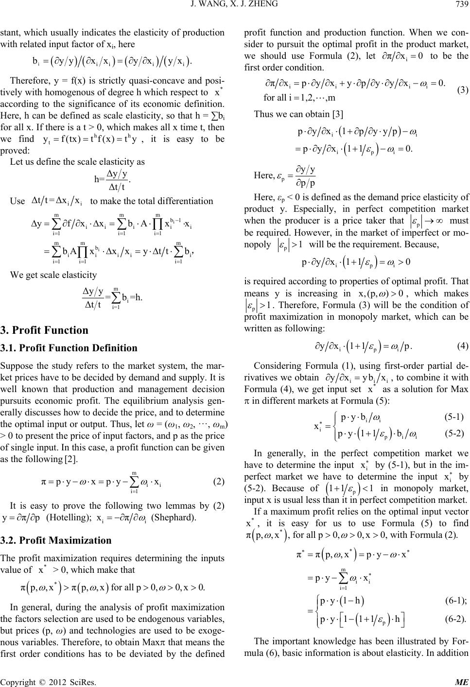
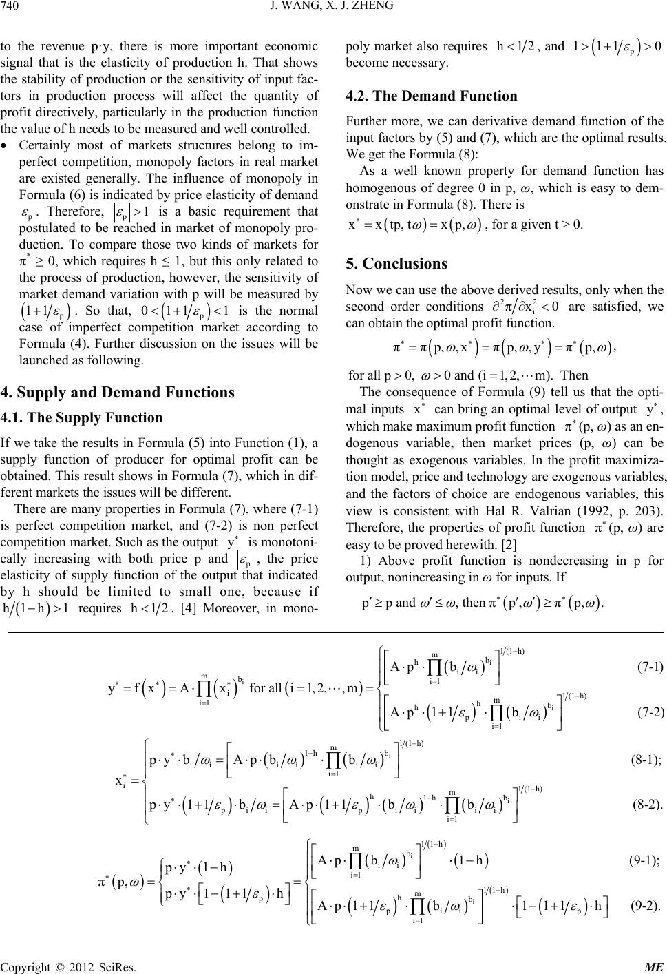
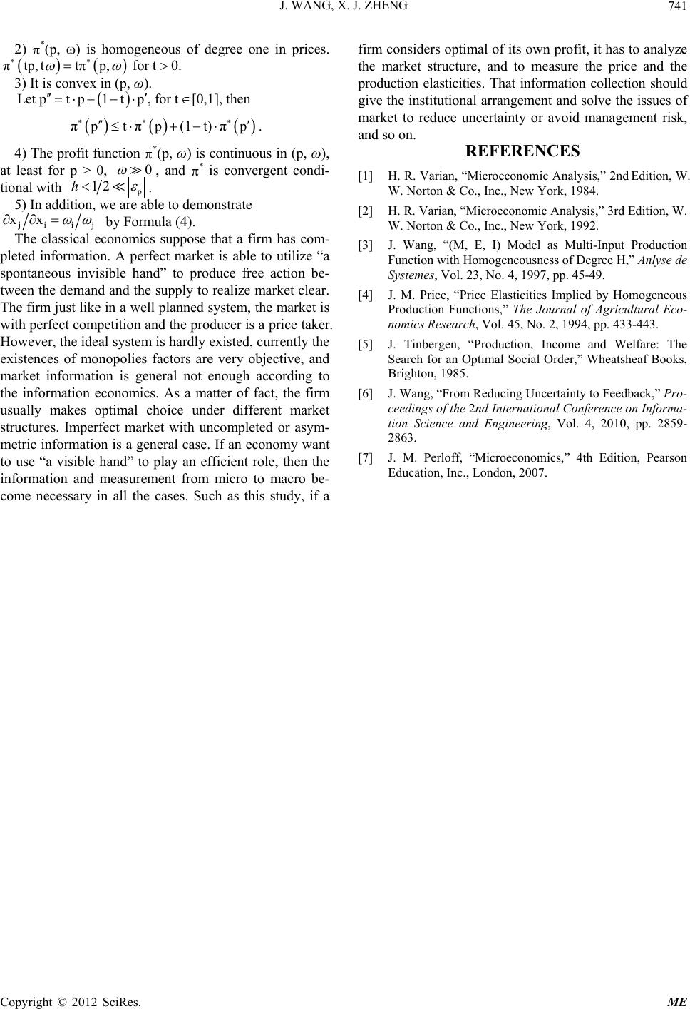
Modern Economy, 2012, 3, 738-741

http://dx.doi.org/10.4236/me.2012.36094 Published Online October 2012 (http://www.SciRP.org/journal/me)

Study on the Production Technology, Elasticities and

Market Structure Impact on Profit Formation*

Jian Wang1#, Xuejun Zheng2

1College of Economics and Trade, Agricultural University of Hebei, Baoding City, China

2College of Foreign Language, Agricultural University of Hebei, Baoding City, China

Email: #wangjian@hebau.edu.cn

Received July 5, 2012; revised August 10, 2012; accepted August 20, 2012

ABSTRACT

The size of the profit in a firm or a production system not only depends on the quantity of inputs and outputs, but also

depends on the market structure that means the market is perfect competition or imperfect competition. In general, the

relationship between output and inputs can be defined as the production structure, which is usually decided by produc-

tion technology. Therefore, under the market economy system, the production structure regulation has to follow the

market structure variation. Here we assume that production technology is a C-D function, and then to determine the

effects of different market structures, which we find, they are in close contacted with both production and market struc-

tures, especially some variations of elasticities. Through out a series of deduction and equilibrium analysis, the re-

stricted conditions of the maximum profit have been found. Therefore, the consequences show that the values of elastic-

ities have taken an important role in profit obtained for producer, the profits in a perfect competition market hardly de-

pends on market demand elasticity, in which production elasticity requires rather small. However, in the imperfect

competition market, monopoly make both price of demand and production elasticities impact on the profit. Those also

prove that market monopoly factors make production lose efficiency, or lead to the market failure. In the actual process

of production and management, production elasticities and related market information should be strengthened for

measurement, which will be useful for analysis price fluctuation risk and management decision.

Keywords: Elasticity; Profit Function; Supply & Demand Function; Homogeneous of Degree H

1. Introduction

This study is about the production, market structure and

rules of revenue. Production technology often restricts

the profits obtained by producers. Here mainly refers to

the technical constraints of production elasticity. The

technical restriction is usually a production structural

problem, when considering the issue occurred in the

market and market structure will be in close contact with

it. In the production process, technology determines the

conversion of material and market structure makes this

transition become more complicated. Although these pro-

blems have been concerned by economists many years

ago, such as Harold Hotelling (1929), P. A. Samuelson

(1947), Jan Tinbergen (1959), Ragnar Frisch (1965), R.

Shephard (1970, 1981), Thomas J. Lutton and W. Erwin

Diewert (1982), Hal R. Varian (1984, 1997), etc. These

theories may include the production function, theory of

market and profit, and so on. However, many problems

generally exist in reality, which need to prove their seri-

ousness in theory and give more intuitive explanation. So

that we discuss those problems beginning with a homo-

geneous production function defined by the Hal R. Var-

ian (1984, p. 179), and attempt to demonstrate these is-

sues clearly.

2. Definition of Production Function

The Cobb-Douglas technology describes can easily be

extended to the case of m inputs. A generalized C-D fun-

ction for a production process can be defined as follow-

ing [1].

 

yfxAx i1,2,m

orlogylog Ablogx.



 









(1)



Here,



x=x ,x,L,x0

12 m that is a vector with m-

dimensional input factors. y > 0 is a single output of the

production, and f is the function with twice different-

tiable and continuous. That A means technical coefficient

is used to keep in constant. bi is also a quantity of con-

*This paper is supported by China social science university humanity

roject (No. 12YJAZH138).

#Corresponding author.

J. WANG, X. J. ZHENG 739

stant, which usually indicates the elasticity of production

with related input factor of xi, here



iiii i

yyx xy xyx .

tf(x)ty

Therefore, y = f(x) is strictly quasi-concave and posi-

tively with homogenous of degree h which respect to

according to the significance of its economic definition.

Here, h can be defined as scale elasticity, so that h = ∑bi

for all x. If there is a t > 0, which makes all x time t, then

we find , it is easy to be

proved:

yf(tx)

Let us define the scale elasticity as

Δyy

h= .

Δtt

Use ii

Δtt=Δxx

to make the total differentiation

mb1

i i

Axx

ii i

i1 i1

iii

i1 i1

yfxxb

Ax xx





 





ytt b







 







，

We get scale elasticity

i=1

=b=h.

tt 

3. Profit Function

3.1. Profit Function Definition

Suppose the study refers to the market system, the mar-

ket prices have to be decided by demand and supply. It is

well known that production and management decision

pursuits economic profit. The equilibrium analysis gen-

erally discusses how to decide the price, and to determine

the optimal input or output. Thus, let ω = (ω1, ω2, ···, ωm)

> 0 to present the price of input factors, and p as the price

of single input. In this case, a profit function can be given

as the following [2].



py x





 

 (2)

It is easy to prove the following two lemmas by (2)

yπp (Hotelling); xπ (Shephard).



 

3.2. Profit Maximization

The profit maximization requires determining the inputs

value of > 0, which make that



πp,,xπ

,, xforallp



0,0, x0



.

In general, during the analysis of profit maximization

the factors selection are used to be endogenous variables,

but prices (p, ω) and technologies are used to be exoge-

nous variables. Therefore, to obtain Max that means the

first order conditions has to be deviated by the defined

profit function and production function. When we con-

sider to pursuit the optimal profit in the product market,

we should use Formula (2), let i

πx0  to be the

first order condition.

ii ii

πxpyx ypyyx0.

for all i1,2,,m





 

 (3)

Thus we can obtain [3]







ipi

pyx1pyyp





yx110.





 

Here,







Here, εp < 0 is defined as the demand price elasticity of

product y. Especially, in perfect competition market

when the producer is a price taker that p must

be required. However, in the market of imperfect or mo-

nopoly





will be the requirement. Because,









ipi

yx 110





 

x,(p,)0

is required according to properties of optimal profit. That

means y is increasing in



, which makes

p. Therefore, Formula (3) will be the condition of

profit maximization in monopoly market, which can be

written as following:









ipi

yx 11p



 . (4)

Considering Formula (1), using first-order partial de-

rivatives we obtain iii

yx ybx





, to combine it with

Formula (4), we get input set * as a solution for Max

 in different markets at Formula (5)



pii

yb (5-1)

y11b (5-2)











 





x

In generally, in the perfect competition market we

have to determine the input i by (5-1), but in the im-

perfect market we have to determine the input i



(5-2). Because of





11 1





p

in monopoly market,

input x is usual less than it in perfect competition market.

If a maximum profit relies on the optimal input vector

, it is easy for us to use Formula (5) to find





,,x, for all p0,0,x0, with Formula (2).











ππp,,xpyx

py x

y 1 h(6-1);

y11 1h(6-2).















 

 







  







The important knowledge has been illustrated by For-

mula (6), basic information is about elasticity. In addition

J. WANG, X. J. ZHENG

740

to the revenue p·y, there is more important economic

signal that is the elasticity of production h. That shows

the stability of production or the sensitivity of input fac-

tors in production process will affect the quantity of

profit directively, particularly in the production function

the value of h needs to be measured and well controlled.

 Certainly most of markets structures belong to im-

perfect competition, monopoly factors in real market

are existed generally. The influence of monopoly in

Formula (6) is indicated by price elasticity of demand



. Therefore, p1



 is a basic requirement that

postulated to be reached in market of monopoly pro-

duction. To compare those two kinds of markets for

* ≥ 0, which requires h ≤ 1, but this only related to

the process of production, however, the sensitivity of

market demand variation with p will be measured by





. So that,



01

y



1 1



 is the normal

case of imperfect competition market according to

Formula (4). Further discussion on the issues will be

launched as following.

4. Supply and Demand Functions

4.1. The Supply Function

If we take the results in Formula (5) into Function (1), a

supply function of producer for optimal profit can be

obtained. This result shows in Formula (7), which in dif-

ferent markets the issues will be different.

There are many properties in Formula (7), where (7-1)

is perfect competition market, and (7-2) is non perfect

competition market. Such as the output is monotoni-

cally increasing with both price p and



, the price

elasticity of supply function of the output that indicated

by h should be limited to small one, because if



h1h1 requires h12. [4] Moreover, in mono-

poly market also requires h12, and



111 0



 

become necessary.

4.2. The Demand Function

Further more, we can derivative demand function of the

input factors by (5) and (7), which are the optimal results.

We get the Formula (8):

As a well known property for demand function has

homogenous of degree 0 in p, ω, which is easy to dem-

onstrate in Formula (8). There is









xxtp, txp,



, for a given t > 0.

5. Conclusions

Now we can use the above derived results, only when the

second order conditions 22

πx0



 are satisfied, we

can obtain the optimal profit function.







ππp,, xπp,, yπ





 

，

for all p0, 0 and (i1,2,m). Then



 

The consequence of Formula (9) tell us that the opti-

mal inputs



can bring an optimal level of output y



which make maximum profit function (p, ω) as an en-

dogenous variable, then market prices (p, ω) can be

thought as exogenous variables. In the profit maximiza-

tion model, price and technology are exogenous variables,

and the factors of choice are endogenous variables, this

view is consistent with Hal R. Valrian (1992, p. 203).

Therefore, the properties of profit function

π



(p, ω) are

easy to be proved herewith. [2]

1) Above profit function is nondecreasing in p for

output, nonincreasing in ω for inputs. If



pp and , then πp, π







 

 

 



1(1 h)

mbi1

i1(1 h)

i1 hb

pii

Ap b(7-1)

yfxAxfor alli1,2,,m

Ap11b(7-2

)









 











 

 





 











 

1(1h)

1h b

iiiiii

i1(1 h)

h1h b

p iipiiii

ybA pbb(8-1);

y11bAp11bb(8-2).



 

















 



 















 



11h

piip

Apb1h (9-1);

py1 h

πp, py11 1hAp11b111h(9-2).



 















 













 









  









J. WANG, X. J. ZHENG 741

2) *(p, ω) is homogeneous of degree one in prices.



πtp, ttπ



, for t0.





[0,1], then





1t)π



3) It is convex in (p, ω).



Let ptp1tp, for t

 

 

 

πptπp(







 

  .

4) The profit function *(p, ω) is continuous in (p, ω),

at least for p > 0,



, and * is convergent condi-

tional with h



.

5) In addition, we are able to demonstrate

ji ij



 by Formula (4).

The classical economics suppose that a firm has com-

pleted information. A perfect market is able to utilize “a

spontaneous invisible hand” to produce free action be-

tween the demand and the supply to realize market clear.

The firm just like in a well planned system, the market is

with perfect competition and the producer is a price taker.

However, the ideal system is hardly existed, currently the

existences of monopolies factors are very objective, and

market information is general not enough according to

the information economics. As a matter of fact, the firm

usually makes optimal choice under different market

structures. Imperfect market with uncompleted or asym-

metric information is a general case. If an economy want

to use “a visible hand” to play an efficient role, then the

information and measurement from micro to macro be-

come necessary in all the cases. Such as this study, if a

firm considers optimal of its own profit, it has to analyze

the market structure, and to measure the price and the

production elasticities. That information collection should

give the institutional arrangement and solve the issues of

market to reduce uncertainty or avoid management risk,

and so on. REFERENCES

[1] H. R. Varian, “Microeconomic Analysis,” 2nd Edition, W.

W. Norton & Co., Inc., New York, 1984.

[2] H. R. Varian, “Microeconomic Analysis,” 3rd Edition, W.

W. Norton & Co., Inc., New York, 1992.

[3] J. Wang, “(M, E, I) Model as Multi-Input Production

Function with Homogeneousness of Degree H,” Anlyse de

Systemes, Vol. 23, No. 4, 1997, pp. 45-49.

[4] J. M. Price, “Price Elasticities Implied by Homogeneous

Production Functions,” The Journal of Agricultural Eco-

nomics Research, Vol. 45, No. 2, 1994, pp. 433-443.

[5] J. Tinbergen, “Production, Income and Welfare: The

Search for an Optimal Social Order,” Wheatsheaf Books,

Brighton, 1985.

[6] J. Wang, “From Reducing Uncertainty to Feedback,” Pro-

ceedings of the 2nd International Conference on Informa-

tion Science and Engineering, Vol. 4, 2010, pp. 2859-

2863.

[7] J. M. Perloff, “Microeconomics,” 4th Edition, Pearson

Education, Inc., London, 2007.