Modern Economy, 2012, 3, 718-725
http://dx.doi.org/10.4236/me.2012.36092 Published Online October 2012 (http://www.SciRP.org/journal/me)
Optimal Investment Problem with Multiple Risky Assets
under the Constant Elasticity of Variance (CEV) Model
Hui Zhao, Ximin Rong, Weiqin Ma, Bo Gao
School of Science, Tianjin University, Tianjin, China
Received August 15, 2012; revised September 16, 2012; accepted September 27, 2012
ABSTRACT
This paper studies the optimal investment problem for utility maximization with multiple risky assets under the constant
elasticity of variance (CEV) model. By applying stochastic optimal control approach and variable change technique, we
derive explicit optimal strategy for an investor with logarithmic utility function. Finally, we analyze the properties of
the optimal strategy and present a numerical example.
Keywords: Constant Elasticity of Variance Model; Stochastic Optimal Control; Hamilton-Jacobi-Bellman Equation;
Portfolio Selection; Multiple Risky Assets; Stochastic Volatility
1. Introduction
Optimal investment problem of utility maximization is a
fundamental problem in mathematical finance and has
been studied in many articles. This problem is usually
studied via two approaches in literatures. One is stochas-
tic control approach used by Merton [1,2] for the first
time. By this approach, Browne [3] found the optimal
investment strategy to maximize the expected exponen-
tial utility of terminal wealth for an insurance company.
Yang and Zhang [4] studied a similar problem for an
insurer with exponential utility via stochastic control
approach. Another method is the martingale approach
which was adapted to the problem of utility maximiza-
tion by Pliska [5], Karatzas, Lehoczky and Shreve [6]
and Cox and Huang [7]. Much of this development ap-
peared in [8,9]. Applying the martingale approach,
Karatzas et al. [10] investigated the utility maximization
problem in an incomplete market and Zhang [11] con-
sidered a similar problem. In [12], closed-form strategies
were obtained for different utilities maximization of an
insurer through martingale approach. Zhou [13] applied
the martingale approach to study the exponential utility
maximization for an insurer in the Lévy market.
The above mentioned researches using the martingale
method have provided results for general risky assets’
prices, but most found specific solutions for geometric
Brownian motion (GBM) model or a similar one merely.
Meanwhile the works applying stochastic control theory
generally supposed the risky assets’ prices satisfy geo-
metric Brownian motions. However, numerous studies
(see e.g., [14] and the references therein) have shown
that empirical evidence does not support the assumptions
of GBM model and a model with stochastic volatility
will be more practical.
The constant elasticity of variance (CEV) model with
stochastic volatility is a natural extension of geometric
Brownian motion and can explain the empirical bias ex-
hibited by the GBM model, such as volatility smile. The
CEV model allows the volatility to change with the un-
derlying price and was first proposed by Cox and Ross
[15]. In comparison with other stochastic volatility mod-
els, the CEV model is easier to deal with analytically and
the GBM model can be seen as its special case. The CEV
model was usually applied for option pricing and sensi-
tivity analysis of options in most literatures, see [16-19]
for example. Recently, the CEV model has been applied
in the research of optimal investment, as was done by
Xiao, Zhai and Qin [20]. Gao [21,22] investigated the
utility maximization problem for a participant in a de-
fined-contribution pension plan under the CEV model.
Gu, Yang, Li and Zhang [23] used the CEV model for
studying the optimal investment and reinsurance pro-
blems.
However, the above researches of optimization prob-
lem under the CEV model concerned only one risky asset
and a risk-free asset. But actually, an investor needs to
invest in multiple risky assets to disperse risk and in-
crease his/her profit. Thus, to make the optimization
problem even more realistic, we deal with the investment
problem with a risk-free asset and multiple risky assets
under the CEV model. Although Zhao and Rong [24]
have studied portfolio selection problem with multiple
C
opyright © 2012 SciRes. ME

H. ZHAO ET AL. 719








,0,, ,0Stt Sttn
   
=1
d=dd ,
=1,2,, ,
d
iii ijij
j
St SttStWt
in









T
:=, ,WW W
1n of the stocks are
described by the CEV model
risky assets under the CEV model, they obtained closed-
form solutions only for special model parameters. Where-
as in this paper, considering to maximize the expected
logarithmic utility of an investor’s terminal wealth, we
derive optimal strategy explicitly for all values of the
elasticity coefficient. By applying the methods of sto-
chastic optimal control, we derive a complicated nonlin-
ear partial differential equation (PDE). However, there
are terms that contain variables concerning different as-
sets’ prices, which makes it difficult to characterize the
solution structure. Therefore, we conjecture a correspond-
ing solution to this PDE via separating variables partially
and simplify it into several PDEs. The coefficient vari-
ables of these simplified PDEs are closely correlated and
therefore we use a power transformation and a variable
change technique to solve them.
It is noteworthy that the introduction of multiple risky
assets does give rise to difficulties and this research is
not a routine extension of the case of one risky asset. For
portfolio selection problems concerning risky assets with
the CEV price processes, the characterization of solution
under dimensional case is quite different from one
dimensional case. Owing to the consideration of multiple
risky assets, we conjecture the solution through separat-
ing variables represented different assets’ prices and
combining each price variable with time variable respec-
tively.
n
n
 
0,0Stt
 
0
d,0=1,t S
r
Furthermore, we compare our result with that under
the GBM model and that of one dimensional case. Firstly,
the optimal policy for an investor with logarithmic utility
under the CEV model is similar to that under the GBM
model in form except for a stochastic volatility. Secondly,
our solution is just the result of [20] when there is only
one risky asset. Moreover, we present a numerical simu-
lation to analyze the properties of the optimal strategy
under the CEV model.
This paper proceeds as follows. Section 2 proposes the
utility maximization problem with multiple risky assets
whose prices are driven by the CEV models and provides
the general framework to solve the optimization problem.
In Section 3, we derive the optimal investment strategy
for logarithmic utility function and compare our result
with the previous works. Section 4 provides a numerical
analysis to illustrate our results. Section 5 concludes the
paper.
2. Problem Formulation
We consider a financial market consisting of a risk-free
asset (hereinafter called “bond”) and risky assets
(hereinafter called “stocks”). The price process
of the bond follows

00
d=St rS

t (1)
where is the interest rate. The price processes
(2)
where 1d is a d-dimensional standard
Brownian motion defined on a complete probability
space


 
,, ,P dn


=
i
t and . t is an aug-
mented filtration generated by the Brownian motion with
T, where T is a fixed and finite time horizon.

is the appreciation rate of the ith stock and
. Define and

T
1
:=,, n   

=ij nd 


 
 


1
2
00
00
=,
00 n
St
St
St
St


















St

then


is the instantaneous volatility matrix.
The elasticity parameter

satisfies 0=0 . If


,
the volatility matrix is constant with respect to the stock
prices and Equation (2) reduces to the standard Black-
Scholes model. In addition, we assume that T


n

πtt=1,2, ,
  
T
π:= πt, ,πtt
is
positive definite throughout this paper.
The investor is allowed to invest in those stocks as
well as in the bond. Let i be the money amount
invested in the ith stock at time for in.
Denote by 1n and each




πit
is an


=1,2, ,in


π,0tt
t-predictable process for .
Corresponding to a trading strategy and an
initial capital V, the investor’s wealth process




,0Xt tfollows the dynamics





 

T
T
d= πd
πd
0= ,
n
X
trXttr t
tS tWt
XV









1

T
=1, ,111n
(3)
where is an vector.
n
Suppose that the investor has a utility function U
which is strictly concave and continuously differentiable
on


,


 

. Then the investor aims to


π
E.
max
tUXT

 (4)


By applying the classical tools of stochastic optimal
control, we define the value function as


 
  

 
12
11
π
22
,,,, ,
=E = sup
=,,=,= ,0<<
n
t
nn
Htsss x
UXT Sts
St sSt sXtxtT


(5)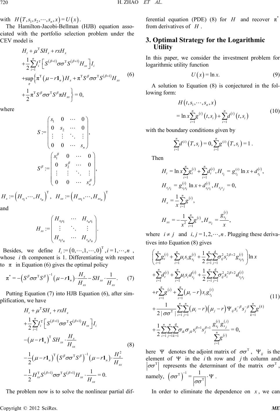

H. ZHAO ET AL. 720



, ,=
with 12 n
,,,
H
Ts ssxUx.
The Hamilton-Jacobi-Bellman (HJB) equation asso-
ciated with the portfolio selection problem under the
CEV model is
 



T
11
TT
=1
TT
TT
1
2
ππ
sup
1ππ=0,
2
tsx
n
is
i
nx
xx
HSHrxH
ISS H
rH S
SSH

















11
T
si
xs
I
S H

 

2
00
00
,
00
00
,
n
n
s
(6)
where
1
2
1
:=
00
:=
00
s
s
S
s
s
S
s




























T
1, ,
ss s
n
H:=HH,


T
1, ,
xs xsn
H
1
.
s s
n
s s
nnn
HH
HH








T
0,=1,,
:=
xs
HH
and
11
1
:=
ss
ss
ss
H
Besides, we define

:=0,,1,,
i
I
in
i
π
 ,
whose th component is 1. Differentiating with respect
to in Equation (6) gives the optimal policy


1
*T
πx
n
1
=.
x
s
x
xxx
SH
H
SS r
H
H


 

1 (7)
Putting Equation (7) into HJB Equation (6), after sim-
plification, we have
 




 
T
11
TT
=1
T
1
TT
11
TT
1
2
1
2
11
2
tsx
n
is
i
x
nxs
xx
2
=0
.
si
x
nn
x
x
I
xs xs xx
HSHrxH
ISS H
H
rSH
H
H
rSS r
H
HSSH H














 



1
1
  1
(8)
The problem now is to solve the nonlinear partial dif-
ferential equation (PDE) (8) for
H
and recover
from derivatives of
*
π
H
.
3. Optimal Strategy for the Logarithmic
Utility
In this paper, we consider the investment problem for
logarithmic utility function


=ln .Ux x (9)
A solution to Equation (8) is conjectured in the fol-
lowing form:






1
=1 =1
,,,,
=ln ,,
n
nn
ii
ii
ii
Htss x
x
gts dts


 
() ()
=1 =1
,=0,,=1
nn
ii
ii
ii
dTs gTs

 
 
(10)
with the boundary conditions given by
.
Then



()
=1 =1
=1
2
=1
=ln,= ln,
=ln, =0,
1
=,
1
=,=,
nn i
ii i
tttss s
ii i
ii
ii
ss ss ss ss
iii j ii ii
ni
xi
i
ns
ii
xx xsi
i
H
xgdHgxd
HgxdH
Hg
x
g
HgH
x x






ij where

and . Plugging these deriva-
tives into Equation (8) gives
,=1,2, ,ij n
  
 



 

d222
=1=1=1 =1
d222
=1=1=1 =1
=1 =1
T
=1 =1=1
d
=1=1 =1
1ln
2
1
2
1
2| |
1
2
nn n
ii
i
tiiiji sss
iii
ii ij
nnn
ii i
tii iji sss
iii
ii ij
nn i
iii
si
ii
nnn k
ijijij
ij k
nn
ijk
gsg sgx
dsd sd
rg rsg
rrssg
















 



 
 

 

 

(11)
11
=1
=0,
ij
ss
ij
ikjkijni
i
gg
ss
g




T

denotes the adjoint matrix of here

 , ij

is the
element of

in the ith row and th column and j
T


T
represents the determinant of the matrix



,
namely, 1
T
T
1
=  



In order to eliminate the dependence on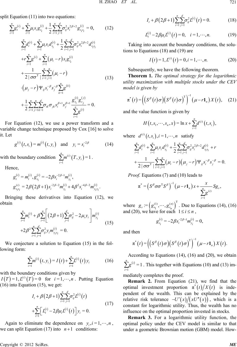
.
x
, we can

H. ZHAO ET AL. 721
split Equation (11) into two equations:
  
=1 =1=1 =1
=0 ,
2
i
ti
i iji
sss
iii
ii ij
gsg sg  
  (12)
22 2
1
nn nd
i
i
 
  






 

22 2
=1
=1
=0 .
nd
ii
iji
=1 =1=1
=1 =1
T
=1 =1
=1
11
=1=1 =1
1
2
1
2| |
1
2
nn
i
tii
s
ss
iii
ij
ij
ss
ij
ni
i
sd
gg
g





(13)
For Equation (12), we use a power transform and a
va
2
and =
ii
ii
nn i
iii
si
ii
nn
i
ij
nk
ji
jij
k
nnd
ikjkij
ijk
dsd
rg rsg
r
rssg
ss



















riable change technique proposed by Cox [16] to solve
it. Let




,= ,
ii
ii
g
tsm tyys

 (14)
with the bounda

() ,=1 ii
mTy.
 242
,
.
i
y
ii
ry condition
=1
n
i

Hence,

i



21
() 22
=,=2
=2 214
ii
tts i
ii
i
s
si
ii i
mg sm
gs







yiyy
ii
msm



Bringing these derivatives into Equation (12), we
ob

2
0.
d
ii
jiiy
i
j
mym 




(15)
We conjecture a solution to Equation (15) in the fol-
lo


=1
ii
ii
i
t Lty

(16)
with the boundary conditions given by
utting Equation
Eget:




2
=1
2=0
di
ti j
ij
ii
i
g
tain



2
=1 =1=1
22
=1 =1
21
2=
nn
ti
ii
nd i
ijiy y
ii
ij
ym







 

wing form:
nn

 
=1
,=
i
mtyI
 
()
=1, =0
i
ITLT for =1, ,in. P
), we
n
(16) intoquation (15


=1
=1
21
n
ti
i
.
I
Lt
ty




(17)
Again to eliminate the ,=1,,
i
yi n,
wtions:

LL






dependence on
e can split Equation (17) into 1n condi
 
2
=1 =1
i
ti
j
ij
 (18)
 

2=0,=1,,.
ii
ti
LLtin   (19)
Taking into account the boundary conditi
tio
21 =0.
nd
ILt  

ons, the solu-
ns to Equations (18) and (19) are




()
=1,=0, =1
i,, .
I
tLti n (20)
Subsequently, we have the following therithmic
ut



orem.
Theorem 1. The optimal strategy for the loga
ility maximization with multiple stocks under the CEV
model is given by
 



 
1
T
n
St rXt


1 (21)
and the value function is given by

()
1
=1
, ,
ni
ni
i
*
π=,tSt



,,, ,=ln
H
tss xxdts

where


() ,,=1,, ii
dtsi n satisfy
  
 
2
=1=1=1 =1
T
=1 =1
1
2
1=0
2| |
ii i
ti
i iji
sss
iii
ii ij
nn
ijijij
ij
dsd dr
rrss








 

Proof. Equations (7) and (10) leads to
22
nn nd
s

 
.


1
*T
π=SS rx

 
1
()
=1
,
ns
ni
i
xSg
g

where


T
(1)( )
1
:=,, n
ss s
n
gg g. Due to Equations (14), (16)
), we have for each
 21 0,
i
y
ii
m
 
and then




and (201in,

=2 =
i
si
gs  



 
1
T
=.
n
tSt rXt


1
According to Equations (14), (16) and (20), we ob
=1
n
i

mediately
21), we find that the
*
πtS
tain

=1
i
g. This together with Equations (10) and (13) im-
completes the proof.
Remark 2. From Equation (
optimal investment proportion
 
*
πtXt is inde-
pendent of the wealth. This caned by the
relative risk tolerance
 
be explain
Ux xUx

, which is a
constant for logarithmic wealth has no
influence on the optimal proportion invested in stocks.
Remark 3. For a logarithmic utility function, the
op
utility. Thus, the
under a geom
timal policy under the CEV model is similar to that
etric Brownian motion (GBM) model. How-

H. ZHAO ET AL. 722
ever, the volatility matrix of the stocks
 
St


is not
constant but related to the prices of stocresult
implies that the CEV model fully consrole of
ks. This
iders the
unidimensional
an


the stochastic price of the stock market.
Remark 4. In the case where there is only one stock
and a bond, i.e . =1n,

,,St  are
d we are back to the settings of [20]. Equation (21)
reduces to
 
*
π=,
r
tXt
2
2St



which is the same as the optimal policy
Zhai and Qin [20]. From Equation (22), we find that
 (22)
derived by Xiao,

*
πt decreases with

. A bigger

means a larger
volatility, which increases risks for investors. Thus, in-
s would reduce thamount invested in the stock to
avoid risks.
4. Numeri
vestore
cal Analysis
me numerical simulations to
optimal strategy and illus-
), i.e.,
n
ks at

In this section, we provide so
analyze the properties of the
trate the dynamic behavior of the optimal strategy.
We assume that there are two stocks and one bond in
the market during the time horizon =10T (years
=2. Throughout the numerical analysis, we use the
optimal proportion invested in stoctime t, i.e.,

*Xt to denote the optimal strategy.
Let
πt

 
12
18.16 12.15
= 0.03,=0.12,0.1,=,
12.03 13.10
=1,0= 13.5,0= 12.5.
r
SS






Figure 1 shows the effects of the appreciation rate 1

on the optimal strategies. As expected, the optimal pro-
portion invested in stock 1 increases with respect to its
appreciation rate 1

. Since multiple stocks are consid-
ered, we can analyze the impact of one stock on the other
stock. From Figure 1, we find that there is an inverse
relationship between 1

and the optimal strategy of
stock 2. This is consistent with intuition. When the ap-
preciation rate of one stock increases constantly, it is
optimal to increase the proportion of wealth in this stock
and reduce investment in the other stock. Furthermore,
Figure 1 also shows that the total proportion invested in
two stocks changes moderately with 1

. This implies
that the influence of one stock’s appreciation rate on the
total investment is not obvious.
In Figure 2, the parameters are given by:

 
12
12
= 0.03,=0.12,0.1,=,
1.5 1.2
=0.4, 0=8,0=6.
r
SS






Figures 2(a) and (b) plot the evolution of the stocks’
prices and the optimal strategy over time under the CEV
model, respectively. Unlike the GBM model, the optimal
proportion invested in each stock under the CEV model
0.02 0.04
0.8
0.06 0.080.10.12 0.140.160.180.2
−0.6
−0.4
−0.2
0
0.2
0.4
Proportion invested in stock 1
Proportion invested in stock 2
Proportion invested in two stocks
0.6
Optimal propotion
μ1
Figure 1. The effect of μ1 on the optimal strategy.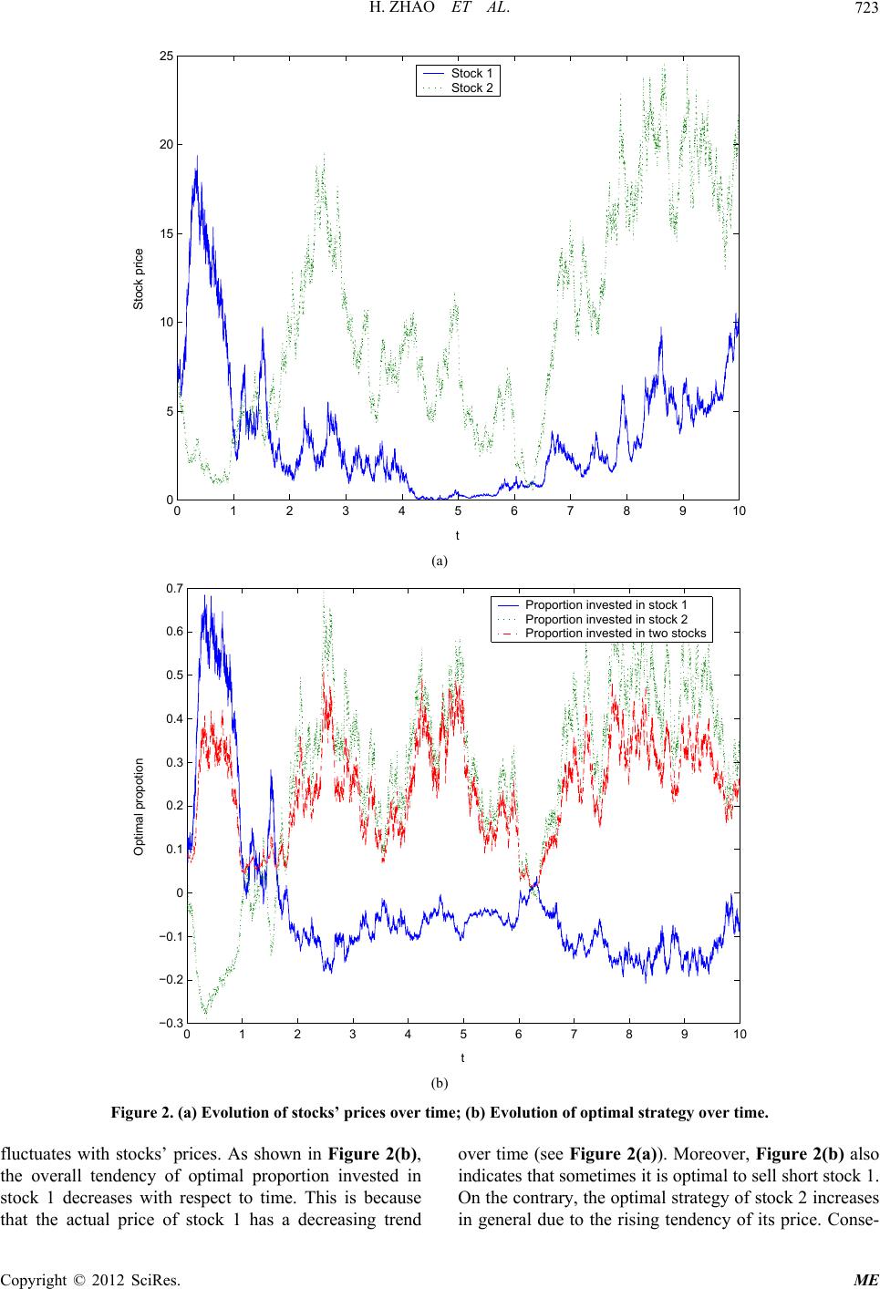

H. ZHAO ET AL. 723
0 1 23 4 5 67 8 91
0
0
5
10
15
20
25
t
Stock price
Stock 1
Stock 2
(a)
0 1 2 3 4 5 6 7 8 910
−0.3
−0.2
−0.1
0
0.1
0.2
0.3
0.4
0.5
0.6
0.7
t
Optimal propotion
Proportion invested in stock 1
Proportion invested in stock 2
Proportion invested in two stocks
(b)
Figure 2. (a) Evolution of stocks’ prices over time; (b) Evolution of optimal strategy over tim.
fluctuates with
the overall tendency of optimal proportion invested in
ure 2(b) also
indicates that sometimes it is optimal to sell short stock 1.
e
stocks’ prices. As shown in Figure 2(b), over time (see Figure 2(a)). Moreover, Fig
stock 1 decreases with respect to time. This is because
that the actual price of stock 1 has a decreasing trend
On the contrary, the optimal strategy of stock 2 increases
in general due to the rising tendency of its price. Conse-

H. ZHAO ET AL. 724
quently, the total proportion invested in stocks is rela-
tively steady over time.
5. Conclusion
By considering multiple risky assets and a risk-free asset
in a financial market, this paper extends the port
der the constant elasticity of vari-
l. We propose the framework of port-
si
d by
n of Tianjin under grant
ts’ innovation training foun-
tainty: The Continuous-Time Case,” The Review of Eco-
nomics and Sta, pp. 247-257.
doi:10.2307/19
folio
selection problem un
ance (CEV) mode
folio selection problem with multiple risky assets under
the CEV model. Explicit solution for the logarithmic
utility maximization has been derived via stochastic con-
trol approach. It is shown that for portfolio selection
problems concerning risky assets with the CEV price
processes, there are differences in solution characteriza-
tion and calculations between one dimensional case and
n dimensional case. The optimal policy under the CEV
model is the same as that under the GBM model in form
except for a stochastic volatility matrix. Finally, numeri-
cal results demonstrate the properties of the multidimen-
onal optimal strategy under the CEV model.
6. Acknowledgements
The authors would be very grateful to referees for their
suggestions and this research was supporte the
Natural Science Foundatio
09JCYBJC01800 and studen
dation of Tianjin University under grant 201210056341.
REFERENCES
[1] R. C. Merton, “Lifetime Portfolio Selection under Uncer-
tistics, Vol. 51, No. 3, 1969
26560
[2] R. C. Merton, “Optimum Consumption and Portfolio
Rules in a Continuous-Time Model,” Journal of Eco-
nomic Theory, Vol. 3, No. 4, 1971, pp. 373-413.
doi:10.1016/0022-0531(71)90038-X
[3] S. Browne, “Optimal Investment Policies for a Firm with
a Random Risk Process: Exponential Utility and Mini-
mizing the Probability of Ruin,” Mathematics of Opera-
tions Research, Vol. 20, No. 4, 1995, pp. 937-958.
doi:10.1287/moor.20.4.937
[4] H. Yang and L. Zhang, “Optimal Investment for Insurer
with Jump-Diffusion Risk Process,” Insurance: Mathe-
matics and Economics, Vol. 37, No. 3, 2005, pp. 615-634.
doi:10.1016/j.insmatheco.2005.06.009
[5] S. Pliska, “A Stochastic Calculus Model of Continuous
Trading: Optimal Portfolios,” Mathematics of Operations
Research, Vol. 11, No. 2, 1986, pp. 371-382.
doi:10.1287/moor.11.2.371
[6] I. Karatzas, J. P. Lehoczky and S. E. Shreve, “Optimal
Portfolio and Consumption Decisions for a ‘Small Inves-
tor’ on a Finite Horizon,” SIAM Journal on Control and
Optimization, Vol. 25, No. 6, 1987, pp. 1557-1586.
doi:10.1137/0325086
[7] J. C. Cox and C. F. Huang, “Optimal Consumption and
Portfolio Policies When Asset Prices Follow a Diffusion
Process,” Journal of Economic Theory, Vol. 49, No. 1,
1989, pp. 33-83. doi:10.1016/0022-0531(89)90067-7
[8] I. Karatzas, “Optimization Problems in the Theory of
Continuous Trading,” SIAM Journal on Control and Op-
timization, Vol. 27, No. 6, 1989, pp. 1221-1259.
doi:10.1137/0327063
[9] I. Karatzas and S. E. Shreve, “Brownian Motion and Sto-
chastic Calculus,” Springer Verlag, New York, 1991.
doi:10.1007/978-1-4612-0949-2
[10] I. Karatzas, J. P. Lehoczky, S. E. Shreve and G. L
“Martingale and Duali
. Xu,
ty Methods for Utility Maximiza-
tion in an Incomplete Market,” SIAM Journal on Control
and Optimization, Vol. 29, No. 3, 1991, pp. 702-730.
doi:10.1137/0329039
[11] A. Zhang, “A Secret to Create a Complete Market from
an Incomplete Market,” Applied Mathematics and Com-
putation, Vol. 191, No. 1, 2007, pp. 253-262.
doi:10.1016/j.amc.2007.02.086
[12] Z. Wang, J. Xia and L. Zhang, “Optimal Investment for
an Insurer: The Martingale Approach,” Insurance: Mathe-
matics and Economics, Vol. 40, No. 2, 2007, pp. 322-334.
doi:10.1016/j.insmatheco.2006.05.003
[13] Q. Zhou, “Optimal Investment for an Insurer in the Lévy
Market: The Martingale Approach,” Statistics & Prob-
ability Letters, Vol. 79, No. 14, 2009, pp. 1602-1607.
doi:10.1016/j.spl.2009.03.027
[14] D. G. Hobson and L. C. G. Rogers, “Complete Models
with Stochastic Volatility,” Mathematical Finance, Vol. 8,
No. 1, 1998, pp. 27-48. doi:10.1111/1467-9965.00043
[15] J. C. Cox and S. A. Ross, “The Valuation of Options f
Alternative Stochastic Process
or
es,” Journal of Financial
Economics, Vol. 3, No. 1-2, 1976, pp. 145-166.
doi:10.1016/0304-405X(76)90023-4
[16] J. C. Cox, “The Constant Elasticity of Variance Option
lasticity
ith Time-Dependent
000814
Pricing Model,” The Journal of Portfolio Management,
Vol. 22, 1996, pp. 15-17.
[17] C. F. Lo, P. H. Yuen and C. H. Hui, “Constant E
of Variance Option Pricing Model w
Parameters,” International Journal of Theoretical and
Applied Finance, Vol. 3, No. 4, 2000, pp. 661-674.
doi:10.1142/S0219024900
[18] D. Davydov and V. Linetsky, “Pricing and Hedging Path-
Dependent Options under the CEV Process,” Manage-
ment Science, Vol. 47, No. 7, 2001, pp. 949-965.
doi:10.1287/mnsc.47.7.949.9804
[19] Y. L. Hsu, T. I. Lin and C. F. Lee, “Constant Elasticity of
Variance (CEV) Option Pricing Model: Integration and
Detailed Derivation,” Mathematics and Computers in
Simulation, Vol. 79, No. 1, 2008, pp. 60-71.
doi:10.1016/j.matcom.2007.09.012
310.
7
[20] J. Xiao, H. Zhai and C. Qin, “The Constant Elasticity of
Variance (CEV) Model and the Legendre Transform-Dual
Solution for Annuity Contracts,” Insurance: Mathematics
and Economics, Vol. 40, No. 2, 2007, pp. 302-
doi:10.1016/j.insmatheco.2006.04.00

H. ZHAO ET AL. 725
[21] J. Gao, “Optimal Portfolios for DC Pension Plans under a
CEV Model,” Insurance: Mathematics and Economics,
Vol. 44, No. 3, 2009, pp. 479-490.
doi:10.1016/j.insmatheco.2009.01.005
[22] J. Gao, “Optimal Investment Strategy for Annuity Con-
tracts under the Constant Elasticity of Variance (CEV)
Model,” Insurance: Mathematics and Economics, Vol. 45,
No. 1, 2009, pp. 9-18.
doi:10.1016/j.insmatheco.2009.02.006
[23] M. Gu, Y. Yang, S. Li and J. Zhang, “Constant Elasticity
of Variance Model for P
vestment Strategies,” Insurance: Math
roportional Reinsurance and In-
ematics and Eco-
nomics, Vol. 46, No. 3, 2010, pp. 580-587.
doi:10.1016/j.insmatheco.2010.03.001
[24] H. Zhao and X. Rong, “Portfolio Selection Problem with
Multiple Risky Assets under the Constant El
Variance Model,” Insurance: Mathema asticity of tics and Econom-
ics, Vol. 50, No. 1, 2012, pp. 179-190.
doi:10.1016/j.insmatheco.2011.10.013
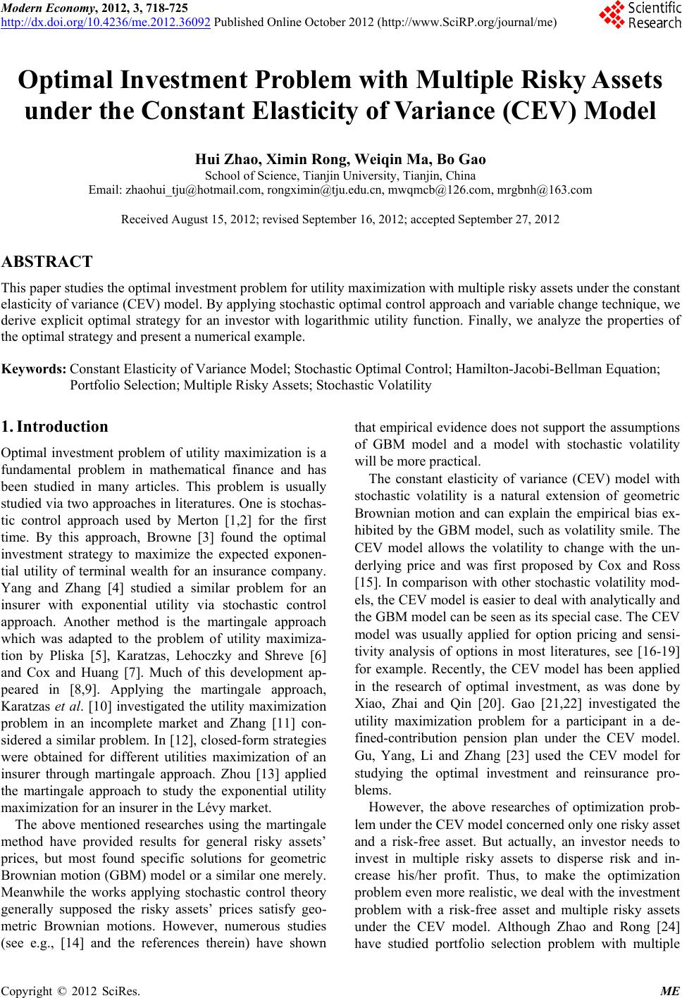