Journal of Transportation Technologies, 2012, 2, 285-296
http://dx.doi.org/10.4236/jtts.2012.24031 Published Online October 2012 (http://www.SciRP.org/journal/jtts)
Temporal Stability and Transferability of Non-Motorized
and Total Trip Generation Models
Judith L. Mwakalonge1*, Juhann C. Waller2, Judy A. Perkins3
1Department of Civil and Mechanical Engineering and Technology, South Carolina State University,
Orangeburg, USA
2Department of Civil and Environmental Engineering, North Carolina A & T State University,
Greensboro, USA
3Department of Civil and Environmental Engineering, Prairie View A & M University, Prairie View, USA
Received June 23, 2012; revised July 21, 2012; accepted August 17, 2012
ABSTRACT
Transportation systems provide a means for moving people and the goods from which they are spatially separated. Of
the two means of surface transportation, the motorized mode is used extensively for utilitarian travel in developed
countries. The increasing reliance on motorized travel has contributed to increased traffic congestion, air pollution, and
greenhouse emissions. Non-motorized travel has recently received significant attention as a means to reduce congestion
and environmental problems and improve human health. However, non-motorized modeling is generally underde-
veloped. This study investigated some changes in non-motorized and total travel and the characteristics of the traveling
public in 1990, 1995, 2001, and 2009 using a national travel survey. The study also investigated the temporal transfer-
ability of linear-regression trip generation models for non-motorized and total travel under such changes. High-income
households made fewer non-motorized trips in 1990 and 1995 compared to 2001 and 2009. Persons aged 50 and over
showed an increased demand for non-motorized travel, whereas children aged 0 - 15 showed a decreasing preference
for non-motorized travel over time. Regarding temporal stability, only the coefficient for single-adult households with
no children was stable across all of the analysis years. For both non-motorized and total travel, most model parameter
estimates were stable short term but not long term. In general, the total travel models transferred better than non-mo-
torized models, both short term and long term. Despite not finding universal stability in model parameter estimates, the
models were marginally able to replicate travel in 2009 relative to the locally estimated 2009 model.
Keywords: Non-Motorized; Transferability; Temporal; Total Travel
1. Introduction
Transportation systems provide a means for moving peo-
ple and the goods from which they are spatially sepa-
rated. There are two means of transportation: motorized
and non-motorized. The motorized segment is mostly
comprised of passenger and freight vehicles that are used
extensively for utilitarian travel in developed countries.
The non-motorized travel segment is mostly comprised
of bicycling and walking, which are not typically used
extensively as means for utilitarian travel in developed
countries. In the US, the use of motorized vehicles as a
means of transportation has been dominant for years and
has been associated with the sprawling land use patterns
in most US cities as well as the relatively low cost of
operating motorized vehicles and nominal parking costs
[1,2]. The increasing reliance on motorized means of
transportation has contributed to increased traffic con-
gestion, air pollution, and greenhouse emissions. The
Urban Transportation Report Card [3] reports that trans-
portation is responsible for 20 to 60 percent of the carbon
emissions in major US cities. Additionally, the Urban
Mobility Report [4] shows that the peak congested hours
increased from 4.5 hours per day in 1982 to 7.1 hours per
day in 2002. The travel time index, which is defined as
the ratio of travel time in rush hour to the travel time
during the free-flow period increased from 1.09 in 1982
to 1.24 in 2007, and wasted fuel per peak traveler in-
creased by 15 gallons during the same period [5]. Fur-
thermore, the report indicates that in 2002, 58 percent of
all major road systems were congested, compared to only
34 percent in 1982. The World Health Organization (WHO)
at the European Region (1999) also reported that auto-
generated pollution is responsible for more deaths than
all traffic accidents. Consequently, more agencies are
seeking or implementing strategies to reduce reliance on
motorized travel.
*Corresponding author.
C
opyright © 2012 SciRes. JTTs

J. L. MWAKALONGE ET AL.
286
Non-motorized travel has recently received significant
attention as a means to reduce congestion and environ-
mental problems and improve human health. Transporta-
tion policymakers view increased non-motorized travel
as a solution to traffic congestion caused by motorized
travel, and politicians view non-motorized travel as an
indicator of community livability. With increased obesity
and related diseases, the public health community views
increased non-motorized travel as an indicator of greater
physical activity, which can be used to explain commu-
nity health levels (Clifton et al. 2004). These reasons and
others have motivated research in non-motorized travel.
In an effort to reduce air pollution resulting from tran-
sportation, the Federal Government enforced the Clean
Air Act Amendments (CAAA) of 1990, which require
Metropolitan Planning Organizations (MPOs) to demons-
trate conformity with the National Ambient Air Quality
Standards (NAAQS) in their transportation development
and investment plans. As a result, several agencies and
communities have considered encouraging non-motori-
zed travel as one of the solutions to mitigate community
problems associated with traffic congestion, air quality,
and human health. For example, the San Francisco Bicy-
cle Coalition is working to transform the city’s streets
and neighborhoods into more livable and safe places for
promoting bicycle transportation [3].
To promote usage of non-motorized travel, transporta-
tion planners and policymakers need to assess the current
usage and identify the benefits of implementing and
improving non-motorized facilities compared to other al-
ternatives. Further, transportation policymakers require a
thorough understanding of non-motorized travel beha-
vior to adequately estimate the impact of policy actions.
However, the literature related to the evaluation of bicy-
cle and pedestrian infrastructure and programs on travel
behavior and emissions is generally underdeveloped [6,7].
Additionally, studies [2,8] indicate the need to collect
accurate data to better understand the behavioral aspects
of non-motorized travel and develop quantitative non-
motorized models.
Most studies [2,9,10] have modeled non-motorized tra-
vel using a single cross-sectional dataset. A study by
Edmond et al. [9] investigated the gender differences in
bicycling behavior using single cross-sectional data col-
lected via an online survey in 2006. Bhat et al. [2] stu-
died non-motorized travel behavior in the San Francisco
Bay Area using a single cross section of data collected in
2000. The use of cross-sectional data for demand model-
ing requires the assumption that surveyed households or
individuals are at the demand-supply equilibrium point at
the time of the survey, and that the travel behavior rela-
tionship established at this equilibrium point remains sta-
ble over time. Forecasting travel with such models means
that variations in travel behavior observed across units
(households or individuals) in the cross section can be
extrapolated over time to predict the travel behavior of
households to account for changes in their demographic
composition. This assumption has been suggested to be
too strong, and empirical studies indicate that travel be-
havior of households of similar composition does not ne-
cessarily remain stable over time.
A wide range of research on trip generation models
with respect to stability and transferability has been con-
ducted, mostly on motorized travel. Kannel and Heath-
ington [11] studied the transferability of two trip fre-
quency models estimated on 1964 cross-sectional data to
predict travel in 1971 in Indianapolis, Indiana (US). Co-
trus et al. [12] studied the transferability of linear-regres-
sion and Tobit trip generation models estimated on 1986
cross-sectional data to 1997 in Israel. The former study
found a shift in auto ownership for selected households,
but overall the models predicted total travel sufficiently
from one period to another in the same region. The latter
study did not find sufficient temporal transferability,
which was due to differences in economic conditions that
existed in the two periods. Furthermore, literature points
out that travel demand is affected by the state of the
economy and the price of oil [13]. For example, studies
in the 1970s [14] indicated that people changed their
travel habits in response to the energy crises that occur-
red during that decade. In addition, most studies have
investigated temporal transferability using only two cross-
sectional datasets. Such studies, though beneficial, may
fall short on accounting for the effects of programs im-
plemented in multiple years. A thorough understanding
of the effect of temporal economy, demographic, and land
use changes over multiple years is im- portant in model-
ing non-motorized travel. Such information would help
planners and policymakers adequately estimate the im-
pact of promoting non-motorized travel in reducing ve-
hicular emissions and traffic congestion. Existence of
temporal stability would help agencies employ the dif-
ferent strategies with less regard to temporal changes.
Further, an investigation on temporal transferability of
non-motorized travel demand models would advance the
understanding of the influence of changes in the urban
structure on non-motorized travel demand, as compared
to total travel demand. Thus, this study had the following
objectives:
 Investigate the change in the relationship between
non-motorized travel, the characteristics of the tra-
veling public, and the surrounding environment.
 Empirically assess the temporal transferability of
non-motorized trip generation models over multiple
years.
 Comparatively analyze the temporal stability of non-
motorized and total trip generation models.
The remainder of this paper is organized as follows:

J. L. MWAKALONGE ET AL.
287
First is a discussion of the data used in this study, fol-
lowed by a descriptive analysis of selected variables as
related to non-motorized travel. The model specification
is then presented. Finally, the results are presented and
discussed, followed by conclusions and recommenda-
tions for future studies.
2. Methodology
2.1. Data
The first set of data used consisted of the 1990 and 1995
National Person Travel Survey (NPTS), which was a
one-day travel survey conducted by the Research Trian-
gle Institute. The 1990 NPTS was conducted between
March 1990 and March 1991 with 21,869 households
and yielded a response rate of 84 percent. The 1995
NPTS was a telephone survey conducted between May
1995 and July 1996 that collected travel information
from more than 42,000 households. The second set of
data used included the National Household Travel Sur-
vey (NHTS) from 2001 and 2009. The 2001 NHTS was a
one-day travel survey that was collected via a telephone
survey by Westat and Morpace from March 2001 to May
2002 and collected travel information from 69,817
households. The 2009 NHTS collected travel information
from more than 150,000 households. Both the 2001 and
2009 NHTS included travel information from household
members aged 0 - 4, which was not done in the previous
surveys. For consistency throughout the analysis, only
the travel information that was common from all data
sets was used in this study. Further, the study used travel
information from households residing within the metro-
politan statistics areas (MSAs). The unit of analysis in
this study was a household since it is believed that most
decisions are made at a household level [15]. Therefore,
the final sample sizes used in this study were 12,494,
29,585, 50,682, and 109,321 for 1990, 1995, 2001, and
2009, respectively. The details of each of these datasets
are well documented on the NHTS website [16].
2.2. Descriptive Analysis
Table 1 shows the changes in travel and selected socio-
economic variables known to influence travel from 1990
to 2009. In all analysis years, the percentage of walk trips
was higher than the percentage of bicycle trips. This may
be attributed to the fact that everyone becomes a pede-
strian at some point throughout the day, but the same
cannot be said about becoming a cyclist. The higher walk
trips may also be attributed to increased walks to gain
transit access [9]. The percentage of motorized trips showed
a marginal decrease, while non-motorized trips increased
marginally from 1990 to 2009. The number of workers
per household was lower in 2009, but the number of ve-
hicles per worker was higher in this same year. This may
be explained by the economic recession that was ongoing
during data collection, which affected the labor market.
The household size, average trip length, and average
daily household trips decreased slightly from 2001 to
2009.
2.3. Distribution of Non-Motorized Trips by Age
and Income Groups
Non-motorized travel involves exertion of physical en-
ergy; therefore, it is expected that the age of the indivi-
dual is likely to influence his or her decision to use non-
motorized modes. Likewise, income may indicate the
ability of a family to own, operate, and maintain a vehi-
cle. Therefore, non-motorized trips were cross-tabulated
with age and income groups, and the frequencies of trips
made by each age and income group are shown in Figure
1.
In general, all else being equal, there was an opposite
change in the non-motorized travel pattern for persons
Table 1. Changes in trip and selected demographic characteristics.
Percent of
non-motorized
trips
Year
Bike Walk
Percent of
motorized
trips
Household
size
Vehicles per
driver
Workers per
household
Vehicles
per worker
Average
trip length
(miles)
Household
trips per day
9.6 90.4
1990
7.46
92.54 2.63 1.11 1.17 1.48 9.47 6.91
12.8 87.2
1995
6.07
93.93 2.59 1.01 1.32 1.31 9.13 9.62
9.3 90.7
2001
8.87
91.13 2.60 1.06 1.37 1.36 10.04 9.56
8.6 91.4
2009
9.47
90.53 2.58 1.06 1.11 1.69 9.33 8.56

J. L. MWAKALONGE ET AL.
288
(a)
Tri p- r at e Di st r i but i on by Househol d Inc ome
Category
0
0. 2
0. 4
0. 6
0. 8
1
1. 2
1. 4
1. 6
1. 8
2
1234567891011 1213 141516 17
income Cate gory
trip rate
2009
2001
1995
1990
(b)
Figure 1. Non-motorized household trip rate by age (a) and
income (b). Note: 1 ≤ $5000, 2 = $5000 - $9999, 3 = $10,000 -
$14,999, 4 = $15,000 - $19,999, 5 = $20,000 - $24,999, 6 =
$25,000 - $29,999, 7 = $30,000 - $34,999, 8 = $35,000 -
$39,999, 9 = $40,000 - $44,999, 10 = $45,000 - $49,999, 11 =
$50,000 - $54,999, 12 = $55,000 - $59,999, 13 = $60,000 -
$64,999, 14 = $65,000 - $69,999, 15 = $70,000 - $74,999, 16 =
$75,000 - $79,999, 17 ≥ $80,000.
aged 39 or less and persons aged 40 or more. Specifically,
non-motorized trips made by the younger group gene-
rally decreased over time, while non-motorized trips of
the older group increased. This may be explained in part
by the increased reliance on using private automobiles,
rather than walking and bicycling, for making school
trips, as reported in Ulfarsson and Shankar [17]. Persons
aged 15 or less made more non-motorized trips than any
other age group in 1990, 1995, and 2001, but this trend
changed in 2009, when persons aged 50 to 59 outpaced
the >15 group by more than 5 percent. Consistent with
other studies, low-income households made more non-
motorized trips compared to other income groups. How-
ever, the high-income households showed a monotonic
increase in making non-motorized trips over time.
2.4. Distribution of Non-Motorized Trips by
Lifecycle
Lifecycle defines the household composition and the
extent of responsibilities a given household encounters.
In general, it is expected that households with children
make more trips than their counterparts. Figure 2 shows
the distribution of non-motorized trips for each lifecycle
category, as defined in Table 2. Households with two or
more adults and children aged 6 to 15 had the highest
percentage of non-motorized trips in 1990 but showed a
decreasing trend over time. This may be explained by the
relative independence of children aged 6 to 15 and thus
the likelihood of them bicycling or walking to school or
to playgrounds and/or parks near their homes [2]. It is
apparent from Figure 2 that single-parent households
made relatively fewer non-motorized trips than dual-
parent households. All else being equal, households with
retired persons showed a monotonic increase in non-
motorized travel. Considering the increase in the aging
population, this may indicate the need for bicycling and
walking facilities for communities with higher popula-
tions of retired persons.
2.5. Model Specification
Several variables contained within the four cross-sec-
tional datasets are known to influence travel behavior.
Thus, an analysis was performed to identify which vari-
ables have a high influence on non-motorized and total
travel, thus specifying a simple but robust model. After
performing an analysis of variance and correlation ratio,
Trip Dis t r ibut ion by Life cyc l e
0
5
10
15
20
25
30
35
12345678910
Life cycle cate go ry
percent
2009
2001
1995
1990
(a)
Trip - Rat e Di str ibution by Life cyc l e
0.0000
0.5000
1.0000
1.5000
2.0000
2.5000
12345678910
l i fecycl e
trip-r at e
2009
2001
1995
1990
(b)
Figure 2. Non-Motorized trip distribution by household life-
cycle.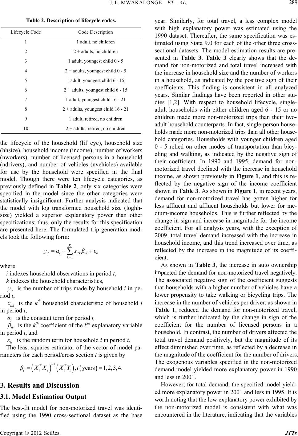

J. L. MWAKALONGE ET AL. 289
Table 2. Description of lifecycle codes.
Lifecycle Code Code Description
1 1 adult, no children
2 2
1
2
2
2
2
+ adults, no children
3 adult, youngest child 0 - 5
4 + adults, youngest child 0 - 5
5 1 adult, youngest child 6 - 15
6 + adults, youngest child 6 - 15
7 1 adult, youngest child 16 - 21
8 + adults, youngest child 16 - 21
9 1 adult, retired, no children
10 + adults, retired, no children
the lifecycle of the househd (lif_cyc), household size
where
xes household observations in period t,
ehold i in pe-
rio
ol
(hhsize), household income (income), number of workers
(nworkers), number of licensed persons in a household
(ndrivers), and number of vehicles (nvehicles) available
for use by the household were specified in the final
model. Though there were ten lifecycle categories, as
previously defined in Table 2, only six categories were
specified in the model since the other categories were
statistically insignificant. Further analysis indicated that
the model with log transformed household size (loghh-
size) yielded a superior explanatory power than other
specifications; thus, only the results for this specification
are presented here. The formulated trip generation mod-
els took the following form:
K
1
it titk tkit
k
yαxβε

 

i inde
k indexes the household characteristics,
it
y is the number of trips made by hous
d t,
itk
x
is the kth household characteristic of household i
in
constant term for period t,
period t,
t
α is the
tk
β
is the kth coefficient of the kth explanatory variable
in
om term for household i in period t.
pa-
ra

travel was identi-
hown in Table 3, the increase in auto ownership
im
tal demand, the specified model yield-
ed
period t, and
it
ε is the rand
The least squares estimator of the vector of model
meters for each period/cross section t is given by

–1

, years1,2,3,4.
TT
ttt tt
βXXXY t
3. Results and Discussion
3.1. Model Estimation Output
The best-fit model for non-motorized
fied using the 1990 cross-sectional dataset as the base
year. Similarly, for total travel, a less complex model
with high explanatory power was estimated using the
1990 dataset. Thereafter, the same specification was es-
timated using Stata 9.0 for each of the other three cross-
sectional datasets. The model estimation results are pre-
sented in Table 3. Table 3 clearly shows that the de-
mand for non-motorized and total travel increased with
the increase in household size and the number of workers
in a household, as indicated by the positive sign of their
coefficients. This finding is consistent in all analyzed
years. Similar findings have been reported in other stu-
dies [1,2]. With respect to household lifecycle, single-
adult households with either children aged 6 - 15 or no
children made more non-motorized trips than their two-
adult household counterparts. In fact, single-person house-
holds made more non-motorized trips than all other house-
hold categories. Households with younger children aged
0 - 5 relied on other modes of transportation than bicy-
cling and walking, as indicated by the negative sign of
their coefficient. In 1990 and 1995, demand for non-
motorized travel declined with the increase in household
income, as shown previously in Figure 1, and this is re-
flected by the negative sign of the income coefficient
shown in Table 3. As shown in Figure 1, in recent years,
demand for non-motorized travel has gotten higher for
less affluent and affluent households but lower for me-
dium-income households. This is further reflected by the
change in sign and increase in magnitude for the income
coefficient. For all analysis years, with the exception of
2009, total travel demand increased with the increase in
household income, and this trend increased over time, as
reflected by the increase in the magnitude of its coeffi-
cient.
As s
pacted the demand for non-motorized travel negatively.
The associated negative sign of the coefficient suggests
that households with a higher number of vehicles have a
lower propensity to take walking or bicycling trips. The
increase in the number of vehicles per driver, as shown in
Table 1, reduced the demand for non-motorized travel,
which is further indicated by the change in sign of the
coefficient for the number of licensed persons in a
household. In contrast, the number of drivers affected the
total travel demand positively, but the magnitude of its
effect diminished over time, as reflected by a decrease in
the magnitude of the coefficient for the number of drivers.
The exogenous variables specified in the non-motorized
demand model yielded more explanatory power in 1990
and less in 2001.
However, for to
more explanatory power in 2001 and less in 1995. It is
worth noting that the low explanatory power exhibited by
the non-motorized model is consistent with what was
encountered in the literature, indicating that the variables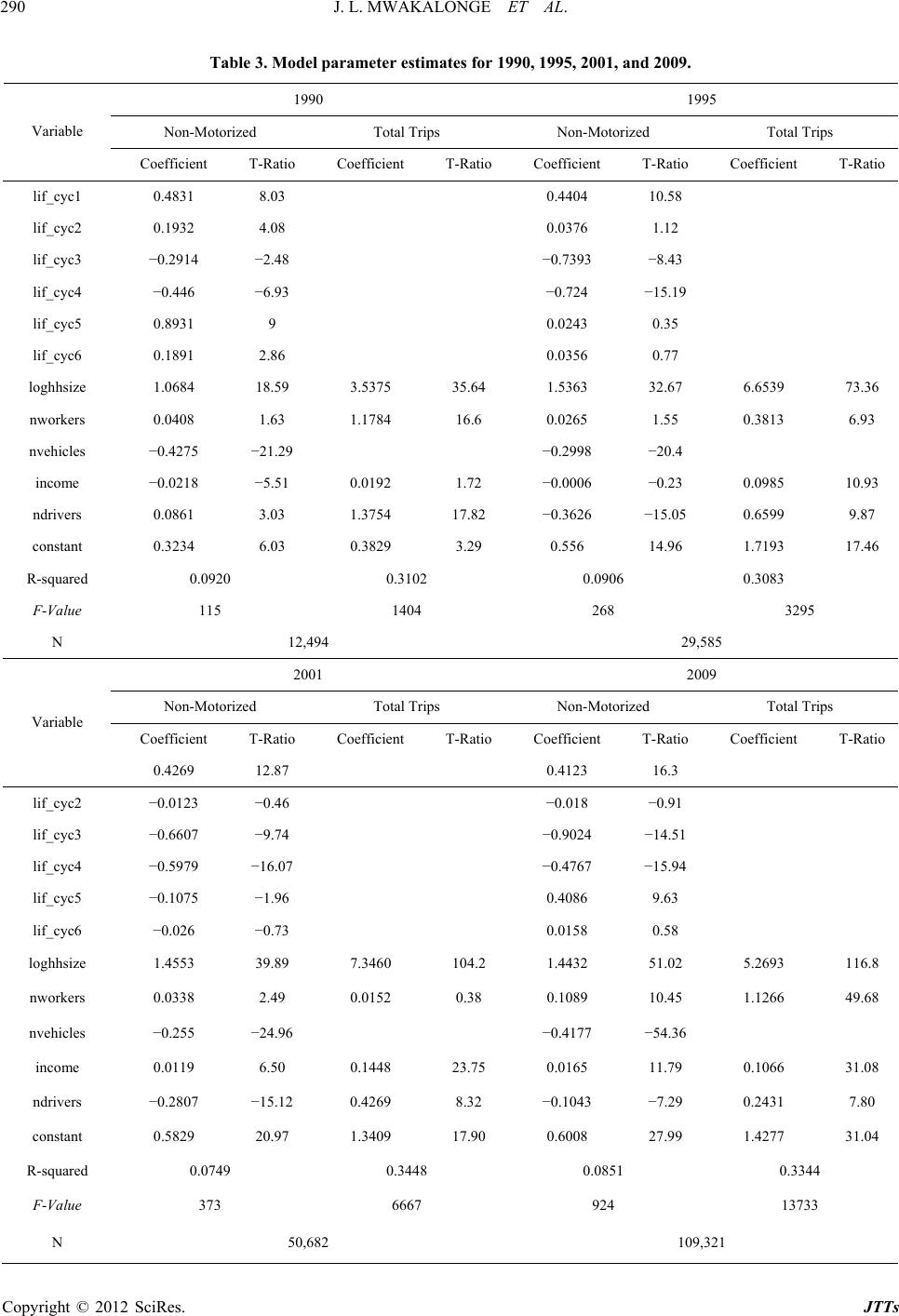

J. L. MWAKALONGE ET AL.
290
tesor 1990, 1995, 2001, and 2009.
1990 1995
Table 3. Model parameter estima f
Non-Motorized Total Trips Non-Motorized Total Trips Variable
CoefCoeffiT-Ratio Coeffficient T-Ratio cient ficient T-Ratio Coeficient T-Ratio
lif_cyc1 0.4831 8.03 0.4404 10.58
lif_cyc2 0.1932 4.08 0.0376 1.12
lif_cyc3 −0.2914 −2.48 −0.7393 −8.43
lif_cyc4 −0.446 −6.93 −0.724 −15.19
lif_cyc5 0.8931 9 0.0243 0.35
lif_cyc6 0.1891 2
loghhsize 3.5375 35.6539 73.
− −−−
0192 1.0985 10.
17. −
0920 3102 0906
295
12,494 29,585
.86 0.0356 0.77
1.0684 18.59 64 1.5363 32.67 6.36
nworkers 0.0408 1.63 1.1784 16.6 0.0265 1.55 0.3813 6.93
nvehicles 0.4275 21.29 0.2998 20.4
income −0.0218 −5.51 0.72 −0.0006 −0.23 0.93
ndrivers 0.0861 3.03 1.3754 82 −0.3626 15.05 0.6599 9.87
constant 0.3234 6.03 0.3829 3.29 0.556 14.96 1.7193 17.46
R-squared 0.0.0.0.3083
F-Value 115 1404 268 3
N
2001 2009
Non-Motorized Total Trips Non-Motorized Total Trips
Coatio CoeffCoRatio Coeff-Ratioefficient T-Ricient T-Ratioefficient T-icient T
Variable
lif_cyc2 − −
0.4269 12.87 0.4123 16.3
0.0123 −0.46 −0.018 0.91
lif_cyc3 −0.6607 −9.74 −−
loghhsize 7.3460 104.2 1.2693 116.8
−−−
0.1448 23.1066 31.
− −−
17.
R-0749 0.3448 0851 0.3344
N 50,682 109,321
0.9024 14.51
lif_cyc4 −0.5979 −16.07 −0.4767 −15.94
lif_cyc5 −0.1075 −1.96 0.4086 9.63
lif_cyc6 −0.026 −0.73 0.0158 0.58
1.4553 39.89 4432 51.02 5.
nworkers 0.0338 2.49 0.0152 0.38 0.1089 10.45 1.1266 49.68
nvehicles −0.255 24.96 0.4177 54.36
income 0.0119 6.50 75 0.0165 11.79 0.08
ndrivers 0.2807 15.12 0.4269 8.32 0.1043 −7.29 0.2431 7.80
constant 0.5829 20.97 1.3409 90 0.6008 27.99 1.4277 31.04
squared 0.0.
F-Value 373 6667 924 13733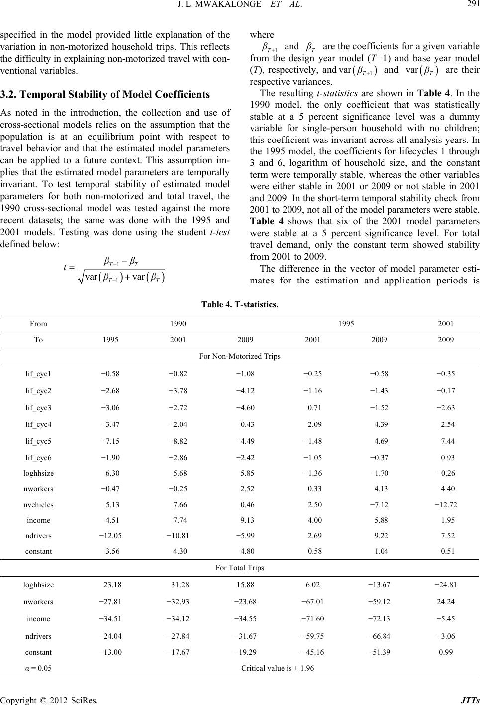

J. L. MWAKALONGE ET AL. 291
specifn the model provided littleation of the
variation in non-motorized household trips. This reflects
bility of Model Coefficients
e

ied i explan
the difficulty in explaining non-motorized travel with con-
ventional variables.
3.2. Temporal Sta
As noted in the introduction, the collection and use of
cross-sectional models relies on the assumption that th
population is at an equilibrium point with respect to
travel behavior and that the estimated model parameters
can be applied to a future context. This assumption im-
plies that the estimated model parameters are temporally
invariant. To test temporal stability of estimated model
parameters for both non-motorized and total travel, the
1990 cross-sectional model was tested against the more
recent datasets; the same was done with the 1995 and
2001 models. Testing was done using the student t-test
defined below:
 
1
1
var var
T+ T
T+ T
ββ
t
β
β



where
1T+
β
and T
β
gn y
ly,
are the coefficients for a given variable
e desiear model (T+1) and base year model
(T
from th
), respective and


1
var T+ β and

var T
β
are their
respective variances.
The resulting t-stati hown 4. In the
1990 model, the only co
stics are sin Table
efficient that was statistically
st
ation and application periods is
Table 4. T-s
From 1990 1995 2001
able at a 5 percent significance level was a dummy
variable for single-person household with no children;
this coefficient was invariant across all analysis years. In
the 1995 model, the coefficients for lifecycles 1 through
3 and 6, logarithm of household size, and the constant
term were temporally stable, whereas the other variables
were either stable in 2001 or 2009 or not stable in 2001
and 2009. In the short-term temporal stability check from
2001 to 2009, not all of the model parameters were stable.
Table 4 shows that six of the 2001 model parameters
were stable at a 5 percent significance level. For total
travel demand, only the constant term showed stability
from 2001 to 2009.
The difference in the vector of model parameter esti-
mates for the estim
tatistics.
To 1995 2009 2001 2009 2001 2009
For Non-Morips torized T
lif_cyc1 −0.58 −0.82 −0.25 −0.58 −0.35 −1.08
lif_cyc2 −2.68 −3.78 −4.12 −1.16 −1.43 −0.17
lif_cyc3 −3.06 −2.72 −4.60 0.71 −1.52 −2.63
lif_cyc4 −3.47 −2.04 −0.43 2.09 4.39 2.54
lif_cyc5 −7.15 −8.82 −4.49 −1.48 4.69 7.44
lif_cyc6 −1.90 −2.86 −2.42 −1.05 −0.37 0.93
loghhsize
−
− −
For Ts
6.30 5.68 5.85 −1.36 −1.70 −0.26
nworkers −0.47 −0.25 2.52 0.33 4.13 4.40
nvehicles 5.13 7.66 0.46 2.50 −7.12 12.72
income 4.51 7.74 9.13 4.00 5.88 1.95
ndrivers 12.05 10.81 −5.99 2.69 9.22 7.52
constant 3.56 4.30 4.80 0.58 1.04 0.51
otal Trip
loghhsize 23.18 31.28 6.02 −13.67 −24.81 15.88
nworkers −27.81 −32.93 −23.68 −
α = 0.05 Critical value is ± 1.96
67.01−59.12 24.24
income −34.51 −34.12 −34.55 −71.60 −72.13 −5.45
ndrivers −24.04 −27.84 −31.67 −59.75 −66.84 −3.06
constant −13.00 −17.67 −19.29 −45.16 −51.39 0.99

J. L. MWAKALONGE ET AL.
292
to as the transfer bias. Lfferences mag-
nitudeges in travel behavior and their respective
n Data Using Models
Usua
text; a
modeability to replicate travel in the estimation
arger disignify the
of chan
explanatory variables from the estimation to application
time period. In general, the t-statistics yielded by the
total travel models were larger compared to those yielded
by the non-motorized models.
3.3. Prediction of Non-Motorized and Total
Travel in the Estimatio
Estimated on 1990, 1995, 2001, and 2009
Data
lly, little is known to a modeler about future con-
hence, the modeler selects the best model based on
l’s cap
context. Thus, in this study, the estimated models were
applied to predict non-motorized and total travel, each in
its respective estimation dataset. The Mean Absolute
Error (MAE) and Percent Error (PE) were used to assess
the models’ capability in forecasting travel in the estima-
tion data. The MAE measure has been used by other
studies [18,19]. MAE is calculated as:
1
1
ˆ
N
iii
i
N
i
i
yyw
MAE
w






where
is the observed number of non-motorized trips pro-
by household i,
the predicted number of non-motorized trips pro-
ctor, and
N
s are presented in Table 5, which
sh increased in magni-
tuor total travel,
th
le
6,
ic
Constant
i
y
duced
ˆi yis
duced by household i,
wi is the weighting fa
is the sample size, all in a given year.
The prediction result
ows that the error measure, MAE,
de over time for non-motorized travel. F
e MAE value was lower in 1990 and higher in 1995.
Further analysis was done to identify in which part of
the US the models were unable to predict non-motorized
travel demand. The results, which are presented in Tab
consistently showed that all of the models studied
over-predicted non-motorized travel in the South Central
tion on estimation data.
Coefficient R-Squared MAE
Table 5. Outputs for pred
Model Trip Type
Non-Motorized0.0920 0.911 2.43E-09 1
1990 Total 5.76E-09 1 0.3102 3.747
Non-Motorized −1.06E-09 1 0.0906 0.955
1995 Total 1.85E-08 1 0.3083 4.767
Non-Motorized −1.79E-09 1 0.0749 1.214
2001
Total −1.01E-08 1 0.3448 4.523
Non-Motorized 1.32E-09 1 0.0851 1.396
2009
Total −2.88E-08 1 0.3344 3.912
Table 6d predicted otorized trips byivision for each a year. . Observed antotal non-m dnalysis
Model New Middle East South East Wes Pacific
Observed 212 1118
England Atlantic North
Central
North
Central Atlantic South Central
South
Central
Mountain
West t
738 2241 1235 291 787 163 382
Predicted
1990
Prd 1.
1995
Pr1 1
2001
Pr 3 12009
PE −6.7 0.9 23 40.6 26.8 81.8 51.5 8.5 −11.5
831 1,602 1,426 339 976 305 658 277 978
PE 12.6 −28.5 15.5 16.5 24 87.3 72.2 30.7 −12.5
Observed 3314 8008 1388 389 1196 169 1208 475 1800
edicte4.064 6.775 1,480 426 644314 2.564 375 1.667
PE 22.6 −15.4 6.6 9.4 37.4 85.7 112.3 −21 −7.4
Observed 914 13,862 12,681 1404 5.685 523 1736 1110 4339
edicted 901 12,302 3,256,8405.903 1.060 3.298 1040 4.257
PE −1.4 −11.3 4.5 31.1 3.8 102.8 90 −6.3 −1.9
Observed 1548 13110 3588 3283 26123 961 11110 6321 20955
edicted 1444 13229 44144615 31301747 6829 6858 18551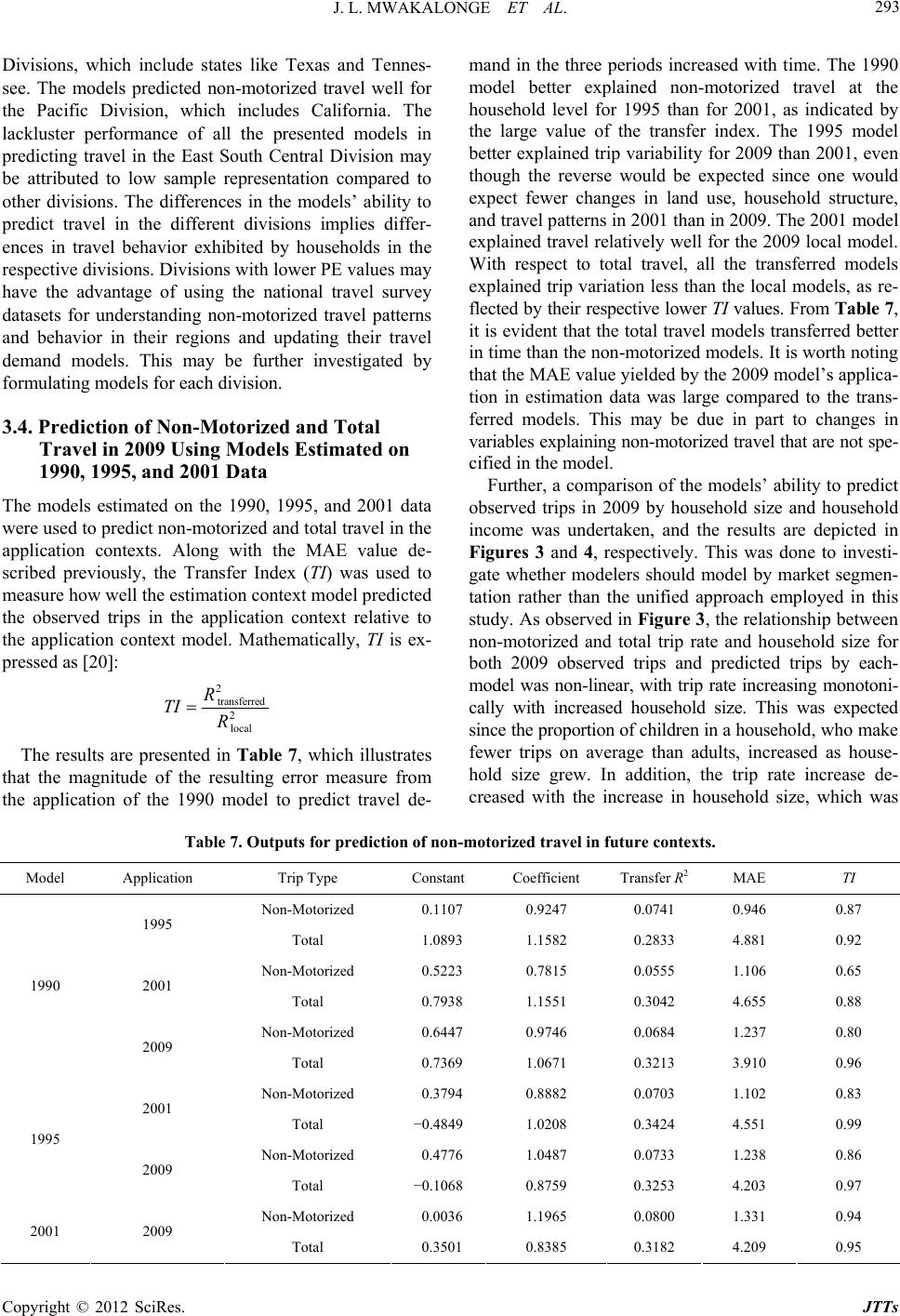

J. L. MWAKALONGE ET AL. 293
Divisionsnclutes lxas
se redicn-md traell fo
the Pacific Division, which includes CaliThe
ckluster prmance of all the presenteddels i
data
appl
scribex (TI) was used to
, which ide staike Teand Tennes-
ee. Thmodels pted nootorizevel w
fornia.
r
la erfo mon
predicting travel in the East South Central Division may
be attributed to low sample representation compared to
other divisions. The differences in the models’ ability to
predict travel in the different divisions implies differ-
ences in travel behavior exhibited by households in the
respective divisions. Divisions with lower PE values may
have the advantage of using the national travel survey
datasets for understanding non-motorized travel patterns
and behavior in their regions and updating their travel
demand models. This may be further investigated by
formulating models for each division.
3.4. Prediction of Non-Motorized and Total
Travel in 2009 Using Models Estimated on
1990, 1995, and 2001 Data
The models estimated on the 1990, 1995, and 2001
were used to predict non-motorized and total travel in the
ication contexts. Along with the MAE value de-
ed previously, the Transfer Ind
measure how well the estimation context model predicted
the observed trips in the application context relative to
the application context model. Mathematically, TI is ex-
pressed as [20]:
2
transferred
2
local
R
TI R 
The results are presented in Table 7, which illustrates
that the magnitude of the resulting error measure from
the application of the 1990 model to predict travel de-
mand in the three periodased wime. T0
model better explainedmotorized travel at the
houseeve1995or 20s indicatby
the lvalue of the trr indexe 199el
pectively. This was done to investi-
ga
-
tant
s increith the 199
non-
than fhold ll for 01, aed
arge ansfe. Th5 mod
better explained trip variability for 2009 than 2001, even
though the reverse would be expected since one would
expect fewer changes in land use, household structure,
and travel patterns in 2001 than in 2009. The 2001 model
explained travel relatively well for the 2009 local model.
With respect to total travel, all the transferred models
explained trip variation less than the local models, as re-
flected by their respective lower TI values. From Table 7,
it is evident that the total travel models transferred better
in time than the non-motorized models. It is worth noting
that the MAE value yielded by the 2009 model’s applica-
tion in estimation data was large compared to the trans-
ferred models. This may be due in part to changes in
variables explaining non-motorized travel that are not spe-
cified in the model.
Further, a comparison of the models’ ability to predict
observed trips in 2009 by household size and household
income was undertaken, and the results are depicted in
Figures 3 and 4, res
Model Application Trip Type Cons
te whether modelers should model by market segmen-
tation rather than the unified approach employed in this
study. As observed in Figure 3, the relationship between
non-motorized and total trip rate and household size for
both 2009 observed trips and predicted trips by each-
model was non-linear, with trip rate increasing monotoni-
cally with increased household size. This was expected
since the proportion of children in a household, who make
fewer trips on average than adults, increased as house-
hold size grew. In addition, the trip rate increase de-
creased with the increase in household size, which was
motorized travel in future contexts.
Coefficient Transfer R2 MAE TI
Table 7. Outputs for prediction of non
Non-Motorized 0.1107 0.9247 0.0741 0.946 0.87
1995
4.881 0.92
Nd 0
2001
Non-zed
1990
2009
Non-zed
2001
Non-zed
1995
2009
Non-zed
2001 2009
Total 1.0893 1.1582 0.2833
on-Motorize 0.5223 0.7815 0.0555 1.106 .65
Total 0.7938 1.1551 0.3042 4.655 0.88
Motori 0.6447 0.9746 0.0684 1.237 0.80
Total 0.7369 1.0671 0.3213 3.910 0.96
Motori 0.3794 0.8882 0.0703 1.102 0.83
Total −0.4849 1.0208 0.3424 4.551 0.99
Motori 0.4776 1.0487 0.0733 1.238 0.86
Total −0.1068 0.8759 0.3253 4.203 0.97
Motori0.0036 1.1965 0.0800 1.331 0.94
Total 0.3501 0.8385 0.3182 4.209 0.95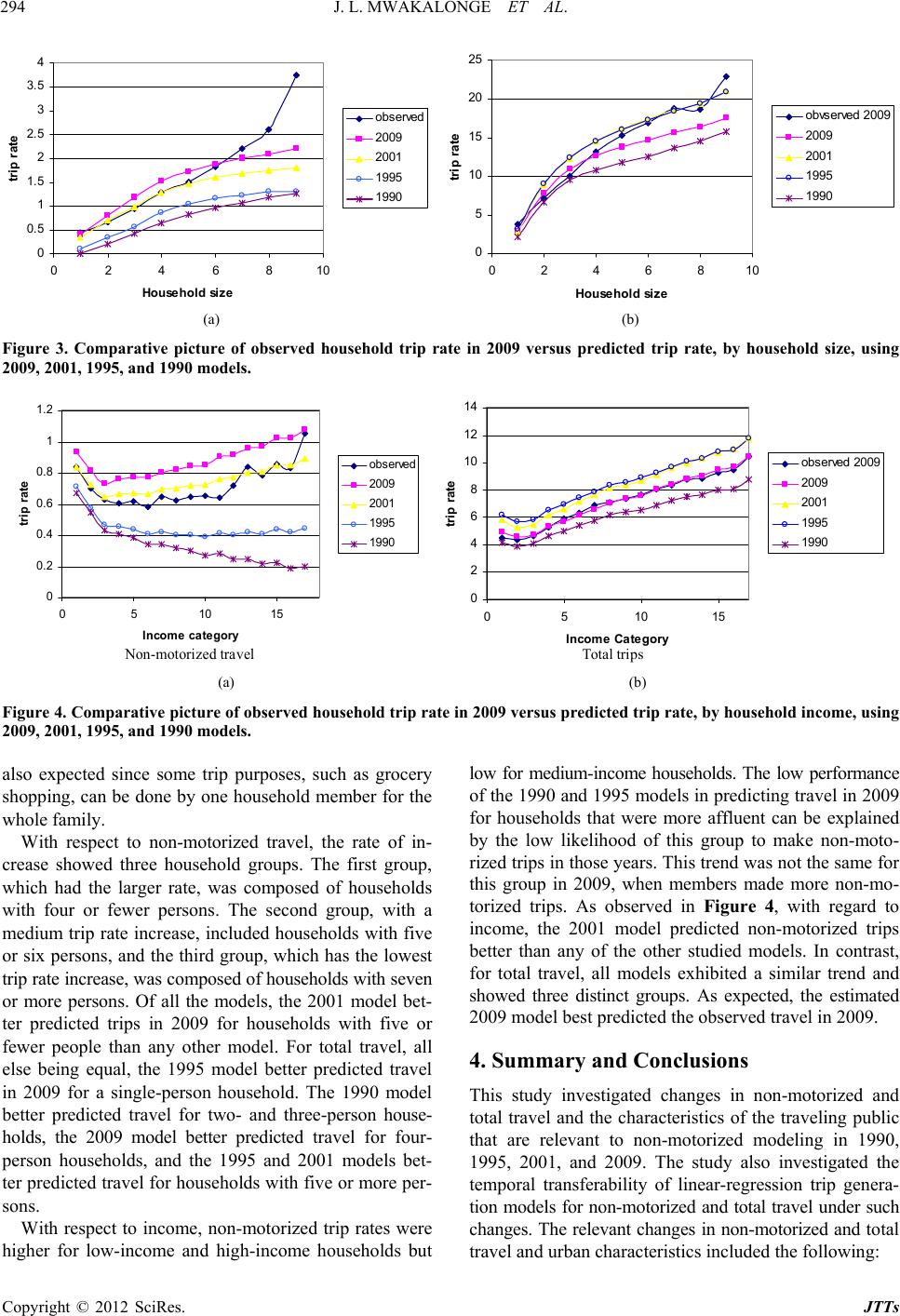

J. L. MWAKALONGE ET AL.
294
0
0. 5
1
1. 5
2
2. 5
3
3. 5
4
0246810
Household siz e
trip r ate
obs erved
2009
2001
1995
1990
0
5
10
15
te
20
25
02468 10
Househol d size
trip ra
obvser9ved 200
2009
2001
1995
1990
(a) (b)
Figure 3. Comparative picture of observed household trip rate in 2009 versus predicted trip rate, by household size, using
2009, 2001, 1995, and 1990 models.
0
0. 2
0. 4
0. 6
0. 8
1
1. 2
051015
Income category
trip rate
obs erved
2009
2001
1995
1990
N
on-motorized travel
0
2
4
6
8
10
12
14
051015
Income Category
tri p rate
obs erved 2009
2009
2001
1995
1990
Total trips
(a) (b)
Figure 4. Comparative picture of observed household trip rate in 2009 versus predicted trip rate, by household income, using
2009, 2001, 1995, and 1990 models.
also expected since some tr
With respect to non-motorized travel, the rate of in-
ewer persons. The second group, with a
m
higher for low-income and high-income households but
seholds. The low performance
by the low likelihood of this group to make non-moto-
l
travel and urban characteristics included the following:
ip purposes, such as grocery low for medium-income hou
shopping, can be done by one household member for the
whole family.
of the 1990 and 1995 models in predicting travel in 2009
for households that were more affluent can be explained
crease showed three household groups. The first group,
which had the larger rate, was composed of households
with four or f
edium trip rate increase, included households with five
or six persons, and the third group, which has the lowest
trip rate increase, was composed of households with seven
or more persons. Of all the models, the 2001 model bet-
ter predicted trips in 2009 for households with five or
fewer people than any other model. For total travel, all
else being equal, the 1995 model better predicted travel
in 2009 for a single-person household. The 1990 model
better predicted travel for two- and three-person house-
holds, the 2009 model better predicted travel for four-
person households, and the 1995 and 2001 models bet-
ter predicted travel for households with five or more per-
sons.
With respect to income, non-motorized trip rates were
rized trips in those years. This trend was not the same for
this group in 2009, when members made more non-mo-
torized trips. As observed in Figure 4, with regard to
income, the 2001 model predicted non-motorized trips
better than any of the other studied models. In contrast,
for total travel, all models exhibited a similar trend and
showed three distinct groups. As expected, the estimated
2009 model best predicted the observed travel in 2009.
4. Summary and Conclusions
This study investigated changes in non-motorized and
total travel and the characteristics of the traveling public
that are relevant to non-motorized modeling in 1990,
1995, 2001, and 2009. The study also investigated the
temporal transferability of linear-regression trip genera-
tion models for non-motorized and total travel under such
changes. The relevant changes in non-motorized and tota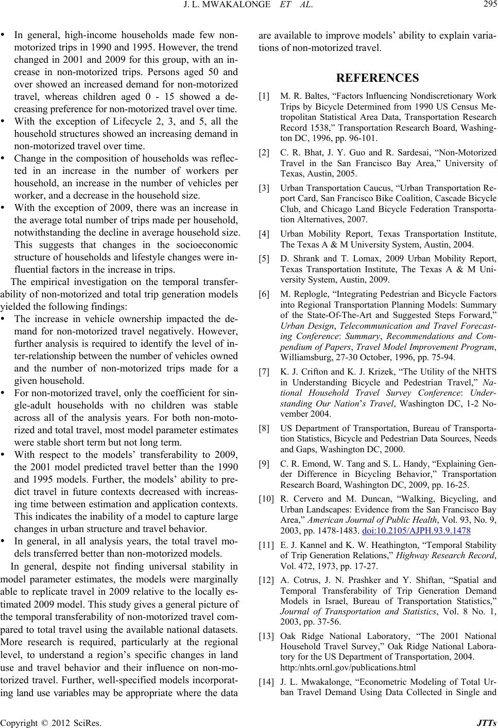

J. L. MWAKALONGE ET AL. 295
 In general, high-income households made few non-

to
ing land use vari
[3] Urban Transportation Caucus, “Urban Transportation Re-
port Card, Sann, Cascade Bicycle
Club, and Chieration Transporta-
ute, The Texas A & M Uni-
rtation Planning Models: Summary
el Model Improvement Program,
HTS
5.
motorized trips in 1990 and 1995. However, the trend
changed in 2001 and 2009 for this group, with an in-
crease in non-motorized trips. Persons aged 50 and
over showed an increased demand for non-motorized
travel, whereas children aged 0 - 15 showed a de-
creasing preference for non-motorized travel over time.
 With the exception of Lifecycle 2, 3, and 5, all the
household structures showed an increasing demand in
non-motorized travel over time.
 Change in the composition of households was reflec-
ted in an increase in the number of workers per
household, an increase in the number of vehicles per
worker, and a decrease in the household size.
 With the exception of 2009, there was an increase in
the average total number of trips made per household,
notwithstanding the decline in average household size.
This suggests that changes in the socioeconomic
structure of households and lifestyle changes were in-
fluential factors in the increase in trips.
The empirical investigation on the temporal transfer-
ability of non-motorized and total trip generation models
yielded the following findings:
 The increase in vehicle ownership impacted the de-
mand for non-motorized travel negatively. However,
further analysis is required to identify the level of in-
ter-relationship between the number of vehicles owned
and the number of non-motorized trips made for a
given household.
For non-motorized travel, only the coefficient for sin-
gle-adult households with no children was stable
across all of the analysis years. For both non-moto-
rized and total travel, most model parameter estimates
were stable short term but not long term.
 With respect to the models’ transferability to 2009,
the 2001 model predicted travel better than the 1990
and 1995 models. Further, the models’ ability to pre-
dict travel in future contexts decreased with increas-
ing time between estimation and application contexts.
This indicates the inability of a model to capture large
changes in urban structure and travel behavior.
 In general, in all analysis years, the total travel mo-
dels transferred better than non-motorized models.
In general, despite not finding universal stability in
model parameter estimates, the models were marginally
able to replicate travel in 2009 relative to the locally es-
timated 2009 model. This study gives a general picture of
the temporal transferability of non-motorized travel com-
pared to total travel using the available national datasets.
More research is required, particularly at the regional
level, to understand a region’s specific changes in land
use and travel behavior and their influence on non-mo-
rized travel. Further, well-specified models incorporat-
ables may be appropriate where the data
are available to improve models’ ability to explain varia-
tions of non-motorized travel.
REFERENCES
[1] M. R. Baltes, “Factors Influencing Nondiscretionary Work
Trips by Bicycle Determined from 1990 US Census Me-
tropolitan Statistical Area Data, Transportation Research
Record 1538,” Transportation Research Board, Washing-
ton DC, 1996, pp. 96-101.
[2] C. R. Bhat, J. Y. Guo and R. Sardesai, “Non-Motorized
Travel in the San Francisco Bay Area,” University of
Texas, Austin, 2005.
Francisco Bike Coalitio
cago Land Bicycle Fed
tion Alternatives, 2007.
[4] Urban Mobility Report, Texas Transportation Institute,
The Texas A & M University System, Austin, 2004.
[5] D. Shrank and T. Lomax, 2009 Urban Mobility Report,
Texas Transportation Instit
versity System, Austin, 2009.
[6] M. Replogle, “Integrating Pedestrian and Bicycle Factors
into Regional Transpo
of the State-Of-The-Art and Suggested Steps Forward,”
Urban Design, Telecommunication and Travel Forecast-
ing Conference: Summary, Recommendations and Com-
pendium of Papers, Trav
Williamsburg, 27-30 October, 1996, pp. 75-94.
[7] K. J. Crifton and K. J. Krizek, “The Utility of the N
in Understanding Bicycle and Pedestrian Travel,” Na-
tional Household Travel Survey Conference: Under-
standing Our Nation’s Travel, Washington DC, 1-2 No-
vember 2004.
[8] US Department of Transportation, Bureau of Transporta-
tion Statistics, Bicycle and Pedestrian Data Sources, Needs
and Gaps, Washington DC, 2000.
[9] C. R. Emond, W. Tang and S. L. Handy, “Explaining Gen-
der Difference in Bicycling Behavior,” Transportation
Research Board, Washington DC, 2009, pp. 16-2
[10] R. Cervero and M. Duncan, “Walking, Bicycling, and
Urban Landscapes: Evidence from the San Francisco Bay
Area,” American Journal of Public Health, Vol. 93, No. 9,
2003, pp. 1478-1483. doi:10.2105/AJPH.93.9.1478
[11] E. J. Kannel and K. W. Heathington, “Temporal Stability
Shiftan, “Spatial and
o. 1,
Collected in Single and
of Trip Generation Relations,” Highway Research Record,
Vol. 472, 1973, pp. 17-27.
[12] A. Cotrus, J. N. Prashker and Y.
Temporal Transferability of Trip Generation Demand
Models in Israel, Bureau of Transportation Statistics,”
Journal of Transportation and Statistics, Vol. 8 N
2003, pp. 37-56.
[13] Oak Ridge National Laboratory, “The 2001 National
Household Travel Survey,” Oak Ridge National Labora-
tory for the US Department of Transportation, 2004.
http:/nhts.ornl.gov/publications.html
[14] J. L. Mwakalonge, “Econometric Modeling of Total Ur-
ban Travel Demand Using Data

J. L. MWAKALONGE ET AL.
296
he Estimation of Trip Generation and
hold
, 2008, pp. 195-206. Repeated Cross-Sectional Surveys,” Ph.D. Dissertation,
Department of Civil and Environmental Engineering, Ten-
nessee Technological University, Cookeville, 2010.
[15] K. G. Goulias, R. M. Pendyala and R. Kitamura, “Practi-
cal Method for t
Trip Chaining,” Transportation Research Board, Washing-
ton DC, 1991, pp. 47-56.
[16] Oak Ridge National Laboratory, “The National House
Travel Survey,” Oak Ridge National Laboratory for the US
Department of Transportation, 2010.
http:/nhts.ornl.gov/publications.html
[17] G. F. Ulfarsson and V. N. Shankar, “Children’s Travel to
School: Discrete Choice Modeling of Correlated Moto-
rized and Non-Motorized Transportation Modes Using
Covariance Heterogeneity,” Environment and Planning B:
Planning and Design, Vol. 35, No. 2
doi:10.1068/b3360
[18] A. Hadayeghi, A. S. Shalaby, B. N. Persaud and C. Cheung,
“Temporal Transferability and Updating of Zonal Level
Accident Prediction Models,” Accident Analysis & Pre-
vention, Vol. 38, No. 3, 2006, pp. 579-589.
doi:10.1016/j.aap.2005.12.003
[19] D. A. Badoe, “An Investigation into the Long Range
erability Ana-
dels,” Transportation Re-
Transferability of Work-Trip Discrete Mode Choice Mo-
dels,” Ph.D. Dissertation, University of Toronto, Toronto,
1994.
[20] F. S. Koppelman and C. G. Wilmot, “Transf
lysis of Disaggregate Choice Mo
search Board, Washington DC, 1982, pp. 18-24.