Open Journal of Statistics, 2012, 2, 383-388
http://dx.doi.org/10.4236/ojs.2012.24046 Published Online October 2012 (http://www.SciRP.org/journal/ojs)
Edgeworth Approximation of a Finite Sample Distribution
for an AR(1) Model with Measurement Error
Shuichi Nagata
Department of Mathematical Sciences, Kwansei Gakuin University, Sanda, Japan
Received July 25, 2012; revised August 27, 2012; accepted September 9, 2012
ABSTRACT
In this paper, we consider the finite sample property of the ordinary least squares (OLS) estimator for an AR(1) model
with measurement error. We present the Edgeworth approximation for a finite distribution of OLS up to O(12 T). We
introduce an instrumental variable estimator that is consistent in the presence of measurement error. Finally, a simula-
tion study is conducted to assess the theoretical results and to compare the finite sample performances of these estima-
tors.
Keywords: Edgeworth Expansion; OLS; Measurement Error; Instrumental Variables Estimator
1. Introduction
The Ordinary Least Squares (OLS) estimator for the AR(1)
model is one of the most general estimators in economet-
rics, and a number of studies considering the properties
of the OLS estimator under certain conditions have been
conducted by several authors. For example, it is well
known that the OLS estimator for the AR(1) model has a
non-negligible bias when the sample size T is not large.
This problem is known as the small sample problem ([1,
2]).
Another problem of the OLS estimator is that the ob-
servation data are sometimes contaminated by noise,
which also affects the estimation result. In this case, the
OLS estimator in the AR(1) model is not consistent. This
problem is commonly known as the measurement error
problem. Following [3] that summarized the early results
on this topic, numerous articles have been published on
this topic. For example, with respect to time series analy-
sis, some estimators in an AR model with measurement
errors in [4] and statistical a test for the existence of
noise is proposed in [5].
In this paper, we deal with these two important prob-
lems simultaneously. In particular, we consider the OLS
estimation when the sample size T is not large, and when
an measurement error is present but ignored. To evaluate
the effect of a small sample size and ignoring measure-
ment error, we derive finite sample properties of the OLS
estimator with noise using the Edgeworth expansion,
which is a traditional technique in econometrics to ap-
proximate a finite sample distribution. For example, the
OLS estimator was studied in [6] for pure AR(1), in [7]
for AR(1) with an unknown mean, and in [8] for AR(1)
with exogenous variables. Following these studies, we
apply the algorithm proposed in [9] to calculate the
Edgeworth coefficients.
In our setting, some problems are the result of noise,
which make calculation difficult. First, if data are af-
fected by noise, it is difficult to obtain variables that are
related to the autocovariance function of the observation
process. To obtain these variables, we use the result in
[10], which shows that an AR(1) process together with
noise can be represented by an ARMA(1, 1) process.
Second, the OLS estimator is inconsistent with noise, and
it is impossible to apply the formula in [9] in this case;
hence we use a corrected error function that follows [8]
and [11] to avoid this problem.
In the simulation section, we also consider a instru-
mental variable (IV) estimation, which is the consistent
estimation in our setting. We compare the finite sample
performances of the OLS estimator with those of our
proposed IV estimator using simulations.
This paper is organized as follows. In the next section,
we provide our setting and the main result for the Edge-
worth approximation of the OLS estimator up to O(12
T).
In Section 3, we examine a Monte Carlo simulation and
graphical comparison. Finally, Section 4 concludes this
paper.
2. Setup and Main Results
We consider a following measurement error model given
by
C
opyright © 2012 SciRes. OJS

S. NAGATA 384


2
2
.0,,
...0,,
u
dN
iidN



1
,~..
,~
ttt t
tttt
yxuuii
xx 


 (1)
where only yt is observable, xt is a stationary AR(1)
process with 1
 
0,1,,tT
and ut is the measurement error or
noise. For a given sample period , the OLS
estimate can be written as follows:
1
2
ˆ,
yCy
yC y




0,, T
(2)
where
y
yy,
12
1
000
2
10
1000 01
2
10
00 200
1
00 0
2
CC

















  

00
00
.
010
00












 
2
The result of this paper relies on the following well
known result given in [10]. If xt is an AR(1) process with
AR parameter β, and ut is white noise with constant
variance


, then yt follows an ARMA(1, 1) process,
which is given by the following equations:

11,
tt
Ly L  

2
~...0,,
t
iidN

 
2
(3)
where L is the lag operator. The parameters


and γ
(the MA parameter) can be related to β, 2


, and 2


as
follows:
2
114
,,
2
q
q


22
u





where
2
22 2
u
u
1
q



 
.
Then, we obtain the following theorem.
Theorem 1. The finite sample distribution of the OLS
estimator up to O(12
T) is given by

 



2
6,
Q Qw 
1
4
32 61
26 1
ˆ
3
Td
pw
iw P
Iw PPP
TPPP










where
 

12
2
12πexp2 ,iww I
 
d
w
wit t




1,, 6
i
Pi

.
12
42
612
PPP  
 
11Prr
ω, and Q are as follows:
,

  
2
212Prr

,


5244334323
3
232 43
22
44
Prrrr r
rr rrr
,

  


 
4233222422
432232Prrrrrr

,

  
343323 324
5
7552443 65
63549 43105 4
5263 74 85 76
65677485 6
783
36263832
61624122616
203212384
862444
3220262432
823,
Prrrrr
rrrr rr
rrrrr
rr rrr
rrrrr
rr
 

 

,



  
 

 


32 4552
6
224233
6524343
635436 354
10 36
3439
449
2643
Pr rrrr
rrrr
rr rr
rrrrr
 
 
 


 
 
  

322
5252413241
612QPPPPPPPP PP   
,
.
Proof. The proof is given in Appendix.
Here, we also examine the IV estimator, which is de-
fined as follows:
2
2
1
2
T
ii
i
T
ii
i
yy
yy







. (4)
The IV estimator is consistent in the presence of the
noise. It is easy to show that the asymptotic variance of
the IV estimator is


22
1


21


. When there is no noise,
the asymptotic variance of the OLS estimator is 1 – β2.
Therefore, the OLS estimator is more efficient than the
IV estimator in the absence of noise.
3. Simulation and Graphical Comparison
In this section, we examine the finite sample property of
the OLS estimator, and evaluate the approximate distri-
bution generated in Section 2 by Monte Carlo simulation.
Data were simulated from Equation (1) with

.
Therefore, the noise-to-signal ratio 22 2



  
throughout this section. In addition to the OLS estimator,
we also compute the IV estimator defined in the previous
section. The number of replications was 20,000. We
computed the mean (Mean) and the root mean squared
error (RMSE) for each estimator. The simulation results
are summarized in Tables 1-3.
From Tables 1-3, we confirm that the OLS estimator
is biased. As expected, the smaller the sample size and

S. NAGATA 385
Table 3. Simulation results (ρ = 0.7). Table 1. Simulation results (ρ = 0.2).
β = 0.4 β = 0.8
Mean RMSE Mean RMSE
T OLS IV OLS IV OLS IV OLSIV
20 0.31 0.91 0.24 68.73 0.68 0.71 0.231.68
40 0.33 0.58 0.17 45.50 0.71 0.75 0.160.22
100 0.34 0.20 0.12 23.74 0.73 0.78 0.110.10
500 0.34 0.40 0.07 0.13 0.74 0.80 0.070.04
800 0.34 0.40 0.07 0.10 0.74 0.80 0.060.03
β = 0.4 β = 0.8
Mean RMSE Mean RMSE
TOLSIVOLSIV OLS IV OLSIV
200.230.620.28109.62 0.56 0.59 0.32 12.6
400.240.990.2272.55 0.60 0.77 0.262.89
1000.250.370.184.39 0.62 0.78 0.20 0.12
5000.250.400.160.18 0.64 0.80 0.17 0.05
8000.250.400.150.14 0.64 0.80 0.17 0.04
the larger the noise variance, the larger will be the bias.
On the other hand, as the IV estimator is a consistent
estimator, IV may converge to the true value. The simu-
lation results are consistent with this hypothesis. How-
ever, in small samples such as for T = 20 and 40, the
RMSE of the IV estimator is rather large, as seen in all
tables.
Table 2. Simulation results (ρ = 0.4).
β = 0.4 β = 0.8
Mean RMSE Mean RMSE
T OLS IV OLS IV OLS IV OLSIV
20 0.27 -0.06 0.25 48.96 0.63 0.69 0.27 3.20
40 0.29 4.23 0.19 540.2 0.66 0.75 0.20 0.29
100 0.29 0.36 0.15 2.53 0.68 0.78 0.150.10
500 0.30 0.40 0.11 0.15 0.70 0.80 0.110.04
800 0.30 0.40 0.11 0.11 0.70 0.80 0.110.03
From the simulation results for the RMSE in Tables 2
and 3, we find that the IV estimator is more efficient than
the OLS estimator when T ≥ 800 (β = 0.4) and T ≥ 100 (β
= 0.8). Therefore, we can conclude that, if the sample
size is not large (T = 20, 40), or both β and ρ are small as
in Table 1 (β = 0.4 and ρ = 0.2), then the OLS estimator
is better than IV in terms of the RMSE.
Next, we compare the exact cdf with the asymptotic
normal distribution. Figure 1 depicts the approximate
distributions of the OLS and the IV with β = 0.4, T = 20,
and various values of ρ. Figure 1 indicates that the OLS
Figure 1. Exact distributions of OLS and IV.

S. NAGATA 386
values have a downward bias. The IV exhibits good be-
havior in the central region of the distribution; however,
its distribution is fatter in the tails compared to the nor-
mal distribution.
Finally, we evaluate the approximate distributions ob-
tained in Section 2, and compare them with the exact cdf
and asymptotic normal distributions. To enable a com-
parison of the shapes of the distributions, the asymptotic
bias of the OLS estimator is corrected hereinafter. Fig-
ure 2 shows the approximate distributions of the OLS
estimator with T = 20, ρ = 0.2, and three different values
of β. From this figure, we can observe the same result as
those obtained in [6]. Figure 3 depicts the approximate
distributions of the OLS with ρ = 0.7, where the other pa-
Figure 2. Exact and approximate distributions of OLS.
0.8
Figure 3. Exact and approximate distributions of OLS.

S. NAGATA 387
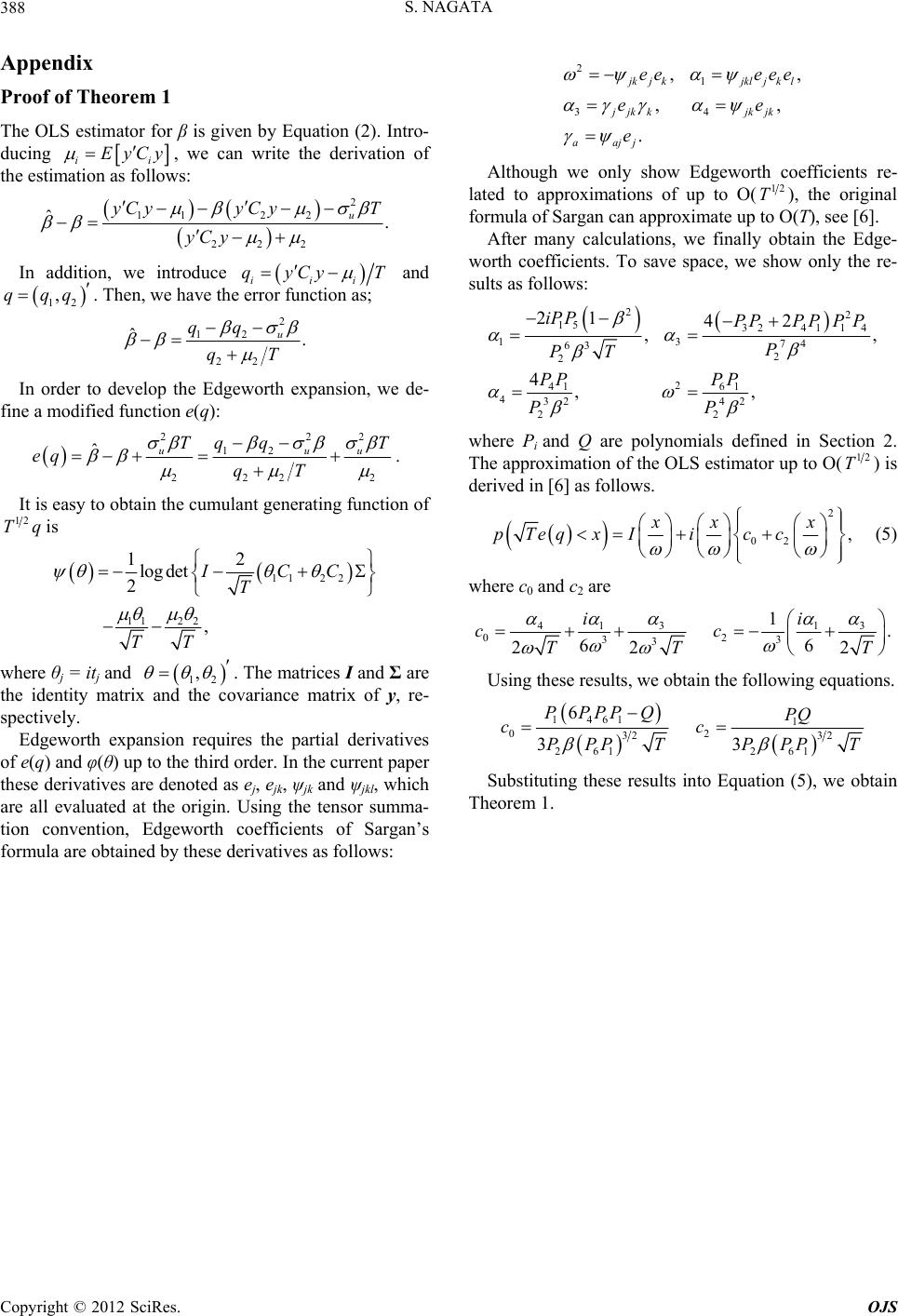
rameter values are the same as those for Figure 2. We
note that the shapes of the distributions are almost the
same, even if the noise ratio ρ is changed. From these
figures, the noise variance has only a small effect on the
shape of the OLS distribution.
4. Discussion
In this paper, we considered finite sample properties of
the OLS estimator for the AR(1) model with measure-
ment error. Using the formula in [9], we obtained the
Edgeworth expansion for finite sample distributions of
the OLS estimator up to O(12 T).
In the simulation work, we have compared naive OLS
estimator with the IV estimator which is a consistent es-
timator in the presence of noise. We can confirm that,
even if the measurement errors is exist, the OLS estima-
tor is more efficient than the IV estimator when the sam-
ple size is small such as T = 20 and 40. If the noise-
to-signal ratio is not so small (ρ ≥ 0.4), the IV estimator
is more efficient than the OLS estimator when T ≥ 800 (β
= 0.4) or T ≥ 100 (β = 0.8). From the graph of the nor-
malized OLS distributions, we find similar properties to
those of the distributions, which correspond to the no
noise situation examined by [6]. This result implies that
measurement error mainly distorts the OLS distributions
for mean and variance; hence we can separately deal with
the two problems of small sample size and observation
errors.
Recently, the differenced-AR(1) estimator was dis-
cussed in [12,13]. Even if the sample size T is relatively
small, this estimator has a small bias. To obtain the finite
sample distribution and to examine the robustness of
such estimators with respect to observation errors, we
can apply the technique of this paper, and this will be
dealt with in a future study.
5. Acknowledgements
I am grateful to Professor Koichi Maekawa for his guid-
ance on this topic and his valuable comments on this
paper. I am also grateful to Professor Yasuyoshi Tokutsu
for his valuable comments.
REFERENCES
[1] F. H. C. Marriott and J. A. Pope, “Bias in the Estimation
of Autocorrelations,” Biometrika, Vol. 41, No. 3-4, 1954,
pp. 390-402. doi:10.2307/2332719
[2] M. G. Kendall, “Note on the Bias in the Estimation of
Autocorrelation,” Biometrika, Vol. 41, No. 3-4, 1954, pp.
403-404. doi:10.2307/2332720
[3] W. A. Fuller, “Measurement Error Models,” John Wiley,
New York, 1987. doi:10.1002/9780470316665
[4] J. Staudenmayer and P. Buonaccorsi, “Measurement Er-
ror in Linear Autoregressive Model,” Journal of the Ameri-
can Statistical Association, Vol. 100, No. 471. 2005, pp.
841-851. doi:10.1198/016214504000001871
[5] K. Tanaka, “A Unified Approach to the Measurement
Error Problem in Time Series Models,” Econometric The-
ory, Vol. 18, No. 2, 2002, pp. 278-296.
doi: 10.1017/S026646660218203X
[6] P. C. B. Phillips, “Approximations to Some Sample Dis-
tributions Associated with a First Order Stochastic Dif-
ference Equation,” Econometrica, Vol. 45, No. 2, 1977,
pp. 463-485. doi.org/10.2307/1911222
[7] K. Tanaka, “Asymptotic Expansions Associated with the
AR(1) Model with Unknown Mean,” Econometrica, Vol.
51, No. 4, 1983, pp. 1221-1231. doi:10.2307/1912060
[8] K. Maekawa “An Approximation to the Distribution of
the Least Squares Estimator in an Autoregressive Model
with Exogenous Variables,” Econometrica, Vol. 51, No.1,
1983, pp. 229-238. doi:10.2307/1912258
[9] J. D. Sargan, “Econometric Estimators and the Edgeworth
Expansions,” Econometrica, Vol. 44, No. 3, 1976, pp.
421-448. doi:10.2307/1913972
[10] C. W. J. Granger and M. J. Morris, “Time Series Model-
ing and Interpretation,” Journal of the Royal Statistical
Society A, Vol. 139, No. 2, 1976, pp. 246-257.
doi:10.2307/2345178
[11] K. Maekawa, “Edgeworth Expansion for the OLS Esti-
mator in a Time Series Regression Model,” Econometric
Theory, Vol. 1, No. 2, 1985, pp. 223-239.
doi:10.1017/S0266466600011154
[12] K. Hayakawa, “A Note on Bias in First-Differenced AR(1)
Models,” Economics Bulletin, Vol. 3 No. 27, 2006, pp. 1-
10.
[13] P. C. B. Phillips and C. Han, “Gaussian Inference in
AR(1) Times Series with or without Unit Root,” Econo-
metric Theory, Vol. 24, No. 3, 2008, pp. 631-650.
doi:10.1017/S0266466608080262

S. NAGATA 388
Appendix
Proof of Theorem 1
The OLS estimator for β is given by Equation (2). Intro-
ducing


ii
, we can write the derivation of
the estimation as follows:
EyCy

 




2
2
2
.
uT 11 2
22
ˆyC yyCy
yC y
 


 


 


In addition, we introduce iii
and
. Then, we have the error function as;
qyCy T 



12
,qqq


2
qq
12
22
ˆ.
u
qT

 
   
In order to develop the Edgeworth expansion, we de-
fine a modified function e(q):

222
2 2
uuu
T
12
22
ˆTq q
eq qT


 

 


.
It is easy to obtain the cumulant generating function of
12
Tq is
 
1122
IC C 

 



,
11 22
12
log det
2
,
T
TT
 
 
 

where θj = itj and 12




2
1
34
,,
,,
.
. The matrices I and Σ are
the identity matrix and the covariance matrix of y, re-
spectively.
j
kjkjkljkl
j jkkjk jk
aajj
ee eee
ee
e
 
 

 


Edgeworth expansion requires the partial derivatives
of e(q) and φ(θ) up to the third order. In the current paper
these derivatives are denoted as ej, ejk, ψjk and ψjkl, which
are all evaluated at the origin. Using the tensor summa-
tion convention, Edgeworth coefficients of Sargan’s
formula are obtained by these derivatives as follows:
Although we only show Edgeworth coefficients re-
lated to approximations of up to O(12 T), the original
formula of Sargan can approximate up to O(T), see [6].
After many calculations, we finally obtain the Edge-
worth coefficients. To save space, we show only the re-
sults as follows:



22
15 324114
13
74
63
2
2
261
41
432 42
22
21 42
,,
4,,
iP PPPPPPP
P
PT
PP
PP
PP






 


where Pi and Q are polynomials defined in Section 2.
The approximation of the OLS estimator up to O(12 T) is
derived in [6] as follows.


2
02 ,
xx x
pTeqxIicc
 


 
 

 
 


(5)
where c0 and c2 are
33 41 1
02
33
3
1
6 6
22 2
ii
cc
TT T

 



 


.
Using these results, we obtain the following equations.


 
1461 1
02
261 26
3
1
32 2
6
33
PPPPQPQ
cc
PPP TPPP T 


Substituting these results into Equation (5), we obtain
Theorem 1.