Open Journal of Statistics, 2012, 2, 420-423
http://dx.doi.org/10.4236/ojs.2012.24051 Published Online October 2012 (http://www.SciRP.org/journal/ojs)
Maximum Likelihood Estimation for Generalized Pareto
Distribution under Progressive Censoring with Binomial
Removals
Bander Al-Zahrani
Department of Statistics, Faculty of Sciences, King Abdulaziz University, Jeddah, Saudi Arabia
Received July 2, 2012; revised August 5, 2012; accepted August 17, 2012
ABSTRACT
The paper deals with the estimation problem for the generalized Pareto distribution based on progressive type-II cen-
soring with random removals. The number of components removed at each failure time is assumed to follow a binomial
distribution. Maximum likelihood estimators and the asymptotic variance-covariance matrix of the estimates are ob-
tained. Finally, a numerical example is given to illustrate the obtain ed results.
Keywords: Pareto Distribution; Binomial Removal; Progressive Censoring; Maximum Likelihood Estimator
1. Introduction
The generalized Pareto distribution is also known as the
Lomax distribution with two parameters, or the Pareto of
the second type. It can be considered as a mixture distri-
bution. Suppose that a random variable
X
has an ex-
ponential distribution with some parameter

. Further,
suppose that

itself has a gamma distribution, and
then the resulting unconditional distribution of
X
is
called the Lomax distribution. This distribution has been
extensively used for reliability modeling and life testing,
for details see e.g. Balkema and de Haan [1]. It also has
been used as an alternativ e to the expon ential d istributio n
when the data are heavy tailed, see Bryson [2]. It has
applications in economics, actuarial modeling, queuing
problems and biological sciences, for more details we
refer to Johnson et al. [3].
A random variable
X
is said to have the generalized
Pareto distribution with two parameters, abbreviated as

,XGP

 

;,1, 0,,0.fxx x    
, if it has the probability density function
(pdf)

1   (1)
Here

and

are the shape and scale parameters,
respectively. The survival function (sf) associated to (1)
is given by

;,1, 0Fxx x

   

(2)
The hazard function is
All standard (further probabilistic properties of this
distribution are given, for example, in Arnold [4]).
In life testing, the experimenter does not always ob-
serve the failure times of all components placed on the
test. In such cases, the censored sampling arises. Fur-
thermore, there are some cases in which components are
lost or removed from the test before failure. This would
lead to progressive censoring. Progressive censoring
schemes are very useful in clinical trials and life-testing
experiments. Balakrishnan and Aggarwala [5] provided a
wealth of information on inferences under progressive
censoring sampling. The progressively type-II censored
life test is described as follows. The experimenter puts n
components on test at time zero. The first failure is ob-
served at 1
X
and then 1 of surviving components is
randomly selected and removed. When the ith failure
component is observed at i
R
X
, i of surviving compo-
nents are randomly selected and removed,
R
2,3,, .im

 The experiment terminates when the mth
failure component is observed at m
X
and
m all removed. In this censoring
scheme 12m are all prefixed. However, in
some practical experiments, these numbers cannot be
pre-fixed and they occur at random. Yuen and Tse [6],
Tse and Yuen [7] and Tse et al. [8] considered the esti-
mation problem for Weibull distribution under type-II
progressive censoring with binomial removals. Shuo [9]
studied the estimation problem for two-parameter Pareto
distribution b ased on progressive censoring with unifor m
removals. Wu [10] provided estimation for the two-pa-
rameter Pareto distribution under progressive censoring
1i
m
i
Rnm R

 

,,,RR R
;,1, 0.hxx x     (3)
C
opyright © 2012 SciRes. OJS

B. AL-ZAHRANI 421
with uniform removals. Wu et al. [11] studied the Burr
type XII distribution based on progressively censored
samples with random removals.
This paper is concerned with the estimation problem
of the unknown parameters for the generalized Pareto
distribution based on progressive type-II censoring with
random removals. The number of components removed
at each failure time is assumed to follow a binomial dis-
tribution. In Section 2, we derive the maximum likely-
hood estimators. The asymptotic variance-covariance ma-
trix of the estimates is obtained in Section 3. In Section 3,
numerical examples are given to illustrate the obtained
results.
2. Maximum Likelihood Estimation
Let 12m
X
XX
mnR

,,R r
be the ordered failure times of
mcomponents, where is pre-specified before the
test. At the ith failure, i components are removed
from the test. For progressive censoring with pre-speci-
fied number of number of removals
1111mm
, the likelihood function can
be defined as follows: (see Cohen [12])
RRr

 
1
1;, m i
i
LxR Crfx 




1i
r
i
Fx




1
11
i
m
ir


 




1
ln
1ln1
1
i
i
m
(4)
where
 
11(Crnnrn (5)
Using relations (1), (2) and (3), the log-likelihood
function is given by


1
1
ln; ,ln
ln
i
m
i
LxCr m
x
x





ri1
1
i
ji
nm r




rp
pi r

1
11nmr
p 






Looking at relation (4), it is noted that the relation is
derived conditional on . Each r can be of any
i
integer value between 0 and We assume
that i is a random number and is assumed to follow a
binomial distribution with parameter . This means the
probability that each component leaves will remain the
same, say , and the probability of component
leaving after the ith failure occurs is

11 r
i
nm
PR rp
r




 (6)
and


1
1
1
11
,,
1i
j
nm r
R r
pp


 
 



12ii
r r
1, ,1im
1
1
11
i
iii i
jj
i
i
r
PR rRr
nm r
r










R
i
. Furthermore, we assume that i is
independent of
X
for all i. The joint likelihood funtion
of


12
,,,
m
X
XX X

12
,,,
m
RRRR
and can
be found



where0, for
1
rnmr
 
1
;,, ;,,LxpLxRPRp    (7)


,
P
Rp is the joint probability distribution of where


12
,, ,
m
Rrr r and is given by










11
11
112 2 11
223311
2211 11
(1)()
11
11
,
,,
,,
!1.
!
ii
i
mm
i
mmm m
mmmm
rmnmmir
mm
i
ii i
PRp
PRrRrR r
PRrRrR r
PRrRr PRr
nm pp
nmr r


 

 



 
 
 






2.1. Point Estimation
The maximum likelihood estimators of

and

are
found by maximizing




,
L
;,,xp 
, since
P
Rp
does not involve the parameters

and

. Thus, the
maximum likelihood estimates (MLEs),


ˆ
ˆ,
 of



,

 can be found by solving the following equations:
 
11
ln 1ln 1
0.
m
i
iii
m
i
ln Lm
x
rx 


 



(8)

11
111
0
ii
mm
iii
ii
x
rx ln Lm
x
x




 



ˆ
(9)

the esti mators of

: From (8) and (9), we obtain
 
11ln1
ˆm
ii
i
m
rx




 (10)
and

can be obtained as the solution of the non-linear
equation


 
1
1
1
1
1
1ln1
1
mii
mii
ii
mi
ii
i
rx
mm
f
x
rx
x
x






 





ˆ
(11)
Therefore,

can be obtained as solution of the
nonlinear equation of the form


g

 
 
, where

1
1
1
1
1
() 1
1ln1
1
mii
mii
ii
i
mi
ii
rx
m
gm
x
rx
x
x


















(12)

B. AL-ZAHRANI 422
ˆ
Since

is a fixed point solution of the non-linear
Equation (12), therefore, it can be obtained using an it-
erative scheme as follows

1, jj
g 


ˆ
where

is the jth iterate of

. The iteration proce-
dure should be stopped when1jj

 is sufficiently
small. Once we obtain ˆ

then ˆ

can be obtained
from (10). The MLEs of reliability and hazard function
are



ˆ
ˆ
1
ˆ;,
F
xx

 




and
ˆ;,hx ˆ.
1
ˆ
ˆ
x



ˆ p

,

Similarly, the MLE of p can be found by maxi-
mizing
P
Rp. Independently, the MLE of parameter
p is the solution of

 
1
1
ln ,
1
1
m
i
ir
PRp
pp
mnm
p







1
1
m
i
imir


 

Hence, the MLE of parameter p is
 
1
1
1
1
ˆ1
m
i
i
m
i
i
r
prmnm




 


1
1
m
i
i
mir



2.2. Interval Estimation
We obtain approximate confidence intervals of the para-
meters

and

based on the asymptotic dis-
tribution of the maximum likelihood estimator of the
parameters. Hence, we employ the asymptotic normal
approximation to obtain confidence intervals for the
unknown parameters. We now obtain the asymptotic
Fisher’s information matrix. The observed information
matrix of 

,,p   
,1,2,3
ij ij
I

 , denoted by is I
222
n lnLLL
2
11 12 13
222
21 2223
2
31 3233
222
2
ln l
ln ln ln
ln ln ln
p
I
II
LLL
I
II
p
I
II
LLL
pp p
  
  



  



 
  

 







  

I


where
1113 31
2
m
II

23 32 ,0III

12 211
1
1
m
i
ii
i
x
Ir
x



 




I



1
2
22 22
11
1
m
i
i
ii
x m
Ir
x





 






11
11
33 22
1
1
mm
ii
ii
rm nmmir
Ipp



 

1
111211 12
212221 22
33 33
00
00
00 00
VVI I
VVI I
VI
The variance-covariance matrix may be approximated
as


 

 


 

 

 
V

The asymptotic distribution of the maximum likely-
hood can be written as follows see e.g. Miller [13].


 
3
ˆ
ˆˆ ,, ~0,ppN V  



(14)
Since V involves the parameters

,

and p, we
replace the parameters by the corresponding MLEs in
order to obtain an estimate of V, which is denoted by .
By using (14), approximate 100 confidence
intervals for
ˆ
V

1 %  

,

and p are determined, respectively,
as
211 222 233
ˆ
,ˆˆ
ˆ
,
ˆ
ˆVVZZpZV

 
Z

is the upper where 100 -

th percentile of the stan-
dard normal distribution.
3. Numerical Study
In our study, we firstly generate the numbers of progress-
sive censoring with binomial removals, i,
and then we get the progressive censoring with binomial
removals samples from GP distribution by the Monte-
Carlo method. The steps are:
1, 2,,,ri m
1
1
~i
ij
j
rBinnm r






1) Step 1 Generate a grou p va lue

and
1
1
m
mi
i
rnm r






2) Step 2 Generate m independent 0, 1
,,,WW W
r
U random
variables .
12 m
3) Step 3 For given values of the progressive censor-
ing scheme , set


1
1.
mmi
ir r
ii
VW 


1UVVV
i
4) Step 4 Set 11immmi


,,,UU U

, then
12 m are progressive censoring with binomial
removals samples of size m from

0,1 .U
5) Step 5 Finally, for given values of parameters

and

 

, we set 1111
ii
xF UU
i



 

.
Then,


,,,
12 m
x
xx is the required from progressive
censoring with binomial removals sample of size m from

B. AL-ZAHRANI 423
which led to a considerable improvement of the paper. the GP distribution.
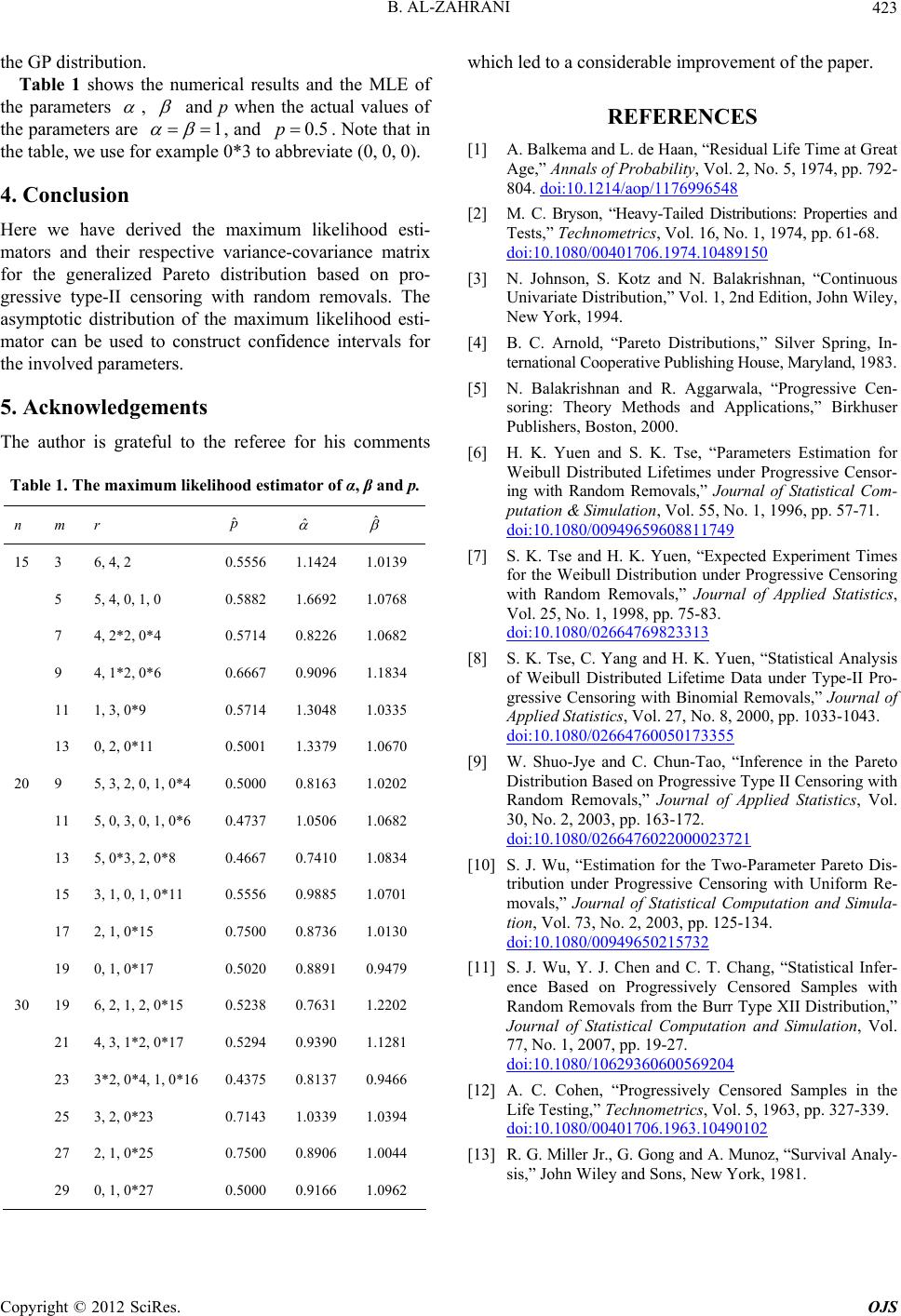
Table 1 shows the numerical results and the MLE of
the parameters

,

and p when the actual values of
the parameters are 1REFERENCES

 
, and . Note that in
the table, we use for example 0*3 to abbreviate (0, 0, 0).
0.5p
ˆ
[1] A. Balkema and L. de Haan, “Residual Life Time at Great
Age,” Annals of Probability, Vol. 2, No. 5, 1974, pp. 792-
804. doi:10.1214/aop/1176996548
4. Conclusion [2] M. C. Bryson, “Heavy-Tailed Distributions: Properties and
Tests,” Technometrics, Vol. 16, No. 1, 1974, pp. 61-68.
doi:10.1080/00401706.1974.10489150
Here we have derived the maximum likelihood esti-
mators and their respective variance-covariance matrix
for the generalized Pareto distribution based on pro-
gressive type-II censoring with random removals. The
asymptotic distribution of the maximum likelihood esti-
mator can be used to construct confidence intervals for
the involved parameters.
[3] N. Johnson, S. Kotz and N. Balakrishnan, “Continuous
Univariate Distribution,” Vol. 1, 2nd Edition, John Wiley,
New York, 1994.
[4] B. C. Arnold, “Pareto Distributions,” Silver Spring, In-
ter nat i ona l C o operat i v e Pub l i s hing Hous e , Mar yl and , 1983.
[5] N. Balakrishnan and R. Aggarwala, “Progressive Cen-
soring: Theory Methods and Applications,” Birkhuser
Publishers, Boston, 2000.
5. Acknowledgements
The author is grateful to the referee for his comments [6] H. K. Yuen and S. K. Tse, “Parameters Estimation for
Weibull Distributed Lifetimes under Progressive Censor-
ing with Random Removals,” Journal of Statistical Com-
putation & Simulation, Vol. 55, No. 1, 1996, pp. 57-71.
doi:10.1080/00949659608811749
Table 1. The maximum likelihood estimator of α, β and p.
ˆ
p
ˆ
n m r


15 3 6, 4, 2 0.5556 1.1424 1.0139
5 5, 4, 0, 1, 0 0.5882 1.6692 1.0768
7 4, 2*2, 0*4 0.5714 0.8226 1.0682
9 4, 1*2, 0*6 0.6667 0.9096 1.1834
11 1, 3, 0*9 0.5714 1.3048 1.0335
13 0, 2, 0*11 0.5001 1.3379 1.0670
20 9 5, 3, 2, 0, 1, 0*4 0.5000 0.8163 1.0202
11 5, 0, 3, 0, 1, 0*6 0.4737 1.0506 1.0682
13 5, 0*3, 2, 0*8 0.4667 0.7410 1.0834
15 3, 1, 0, 1, 0*11 0.5556 0.9885 1.0701
17 2, 1, 0*15 0.7500 0.8736 1.0130
19 0, 1, 0*17 0.5020 0.8891 0.9479
30 19 6, 2, 1, 2, 0*15 0.5238 0.7631 1.2202
21 4, 3, 1*2, 0*17 0.5294 0.9390 1.1281
23 3*2, 0*4, 1, 0*16 0.4375 0.8137 0.9466
25 3, 2, 0*23 0.7143 1.0339 1.0394
27 2, 1, 0*25 0.7500 0.8906 1.0044
29 0, 1, 0*27 0.5000 0.9166 1.0962
[7] S. K. Tse and H. K. Yuen, “Expected Experiment Times
for the Weibull Distribution under Progressive Censoring
with Random Removals,” Journal of Applied Statistics,
Vol. 25, No. 1, 1998, pp. 75-83.
doi:10.1080/02664769823313
[8] S. K. Tse, C. Yang and H. K. Yuen, “Statistical Analysis
of Weibull Distributed Lifetime Data under Type-II Pro-
gressive Censoring with Binomial Removals,” Journal of
Applied Statistics, Vol. 27, No. 8, 2000, pp. 1033-1043.
doi:10.1080/02664760050173355
[9] W. Shuo-Jye and C. Chun-Tao, “Inference in the Pareto
Distribution Based on Progressive Type II Censoring with
Random Removals,” Journal of Applied Statistics, Vol.
30, No. 2, 2003, pp. 163-172.
doi:10.1080/0266476022000023721
[10] S. J. Wu, “Estimation for the Two-Parameter Pareto Dis-
tribution under Progressive Censoring with Uniform Re-
movals,” Journal of Statistical Computation and Simula-
tion, Vol. 73, No. 2, 2003, pp. 125-134.
doi:10.1080/00949650215732
[11] S. J. Wu, Y. J. Chen and C. T. Chang, “Statistical Infer-
ence Based on Progressively Censored Samples with
Random Removals from the Burr Type XII Distribution,”
Journal of Statistical Computation and Simulation, Vol.
77, No. 1, 2007, pp. 19-27.
doi:10.1080/10629360600569204
[12] A. C. Cohen, “Progressively Censored Samples in the
Life Testing,” Technometrics, Vol. 5, 1963, pp. 327-339.
doi:10.1080/00401706.1963.10490102
[13] R. G. Miller Jr., G. Gong and A. Munoz, “Survival A nal y-
sis,” John Wiley and Sons, New York, 1981.