Open Journal of Forestry
2012. Vol.2, No.4, 219-224
Published Online October 2012 in SciRes (http://www.SciRP.org/journal/ojf) http://dx.doi.org/10.4236/ojf.2012.24027
Effect of Spatial Scale on Modeling and Predicting Mean Cavity
Tree Density: A Comparison of Modeling Methods
Stephen S. Lee1, Zhaofei Fan2*
1Department of Statistics, College of Science, University of Idaho, Moscow, USA
2Forest and Wildlife Research Center, Mississippi State University, Starkville, USA
Received June 5th, 2012; revised July 13th, 2012; accepted August 1st, 2012
Cavity trees are integral components of healthy forest ecosystems and provide habitat and shelter for a
wide variety of wildlife species. Thus, monitoring and predicting cavity tree abundance is an important
part of forest management and wildlife conservation. However, cavity trees are relatively rare and their
abundance can vary dramatically among forest stands, even when the stands are similar in most other re-
spects. This makes it difficult to model and predict cavity tree density. We utilized data from the Missouri
Ozark Forest Ecosystem Project to show that it is virtually impossible to accurately predict cavity tree
occurrence for individual trees or to predict mean cavity tree abundance for individual forest stands.
However, we further show that it is possible to model and predict mean cavity tree density for larger spa-
tial areas. We illustrate the prediction error monotonically decreases as the spatial scale of predictions in-
creases. We successfully explored the utility of three classes of models for predicting cavity tree probabil-
ity/density: logistic regression, neural network, and classification and regression tree (CART). The results
provide valuable insights into methods for landscape-scale mapping of cavity trees for wildlife habitat
management, and also on sample size determination for cavity tree surveys and monitoring.
Keywords: CART, Logistic Regression; Neural Network; Oak Forest; Prediction Accuracy
Introduction
Spatial prediction (mapping) of rare forest components such
as cavity trees is an important topic in resource management
and planning intended to conserve wildlife habitat. Cavity trees
are live or dead trees with holes that occur naturally or that are
excavated by certain wildlife species. In Missouri, more than 89
wildlife species require cavity trees or snags (Titus, 1983), and
cavity tree availability is one of the most important factors for
success of populations of cavity-nesting birds (McClelland &
Frissell, 1975).
Extensive analyses regarding factors contributing to cavity
tree formation and abundance prediction in oak forests have
been reported previously (Fan et al., 2003a, 2003b, 2004a,
2004b, 2005). The biggest obstacle in cavity tree prediction for
individual trees, for inventory plots (typically 0.1 to 0.2 ha in
size), and for forest stands (typically 5 to 20 ha in size) results
from the rareness of cavity trees and their large spatial and
temporal variation. This large variation occurs because forma-
tion of cavities is predominately the consequence of a set of
random or semi-random events such as fire, insect attack, dis-
ease, animal excavation, mechanical or chemical injury, and
subsequent decay (Carey, 1983). However, at large spatial
scales cavity tree probability and abundance can be predicted
with reasonable accuracy using tree and stand attributes as in-
dicators of the underlying cavity tree formation processes or
causes (Fan et al., 2004a, 2005).
At the individual tree level, there are numerous statistical
methods such as logistic regression, neural network, and classi-
fication and regression tree (CART) analysis that can be used to
predict the probability that a given tree is a cavity tree and/or to
identify contributing factors associated with cavity abundance.
CART has been shown to be especially promising for estimat-
ing cavity tree abundance at multiple spatial scales (Fan et al.,
2004b, 2005). For cavity tree estimation, CART can explicitly
identify significant contributing tree and/or plot (stand) factors
(and their critical threshold values) and potential interactions in
a hierarchical (nested) structure. CART identifies categories of
observations (nodes) that maximize the separation of cavity
trees from trees without cavities. Nodes quantify cavity tree
probabilities, but they also identify discrete categories that can
be used with aggregation or resampling methods to predict
cavity tree abundance at any spatial scales greater than individ-
ual trees (e.g., plots, stands, small or large landscapes) (Fan et
al., 2004a).
The accuracy of cavity tree abundance or density predictions
made by aggregating individual-tree-level CART models over
plots, stands, or larger spatial scales generally depends on two
factors: 1) how accurately the CART model distinguishes cav-
ity trees from non-cavity trees; and 2) the spatial scale (and
number of cases) over which CART is aggregated. Tradition-
ally, prediction/classification of events of interest (cavity trees
in this study) is accomplished by a single “best” (i.e., most
accurate) model. Recent research suggests that an alternative to
the selection of a single “best” model is to employ ensembles of
models. Breiman (1996) reports that “bootstrap-aggregated”
combinations of models (called Bagged models below) built
from different re-sampled (with replacement) versions of the
original data set, may have significantly lower errors than the
single “best” model, particularly when the models like neural
network and CART are unstable in the sense that different
*Corresponding author.

S. S. LEE, Z. F. FAN
re-sampled versions of the original data set will result in models
that are substantially different.
The objective of this study was to compare the predic-
tion/classification accuracy of binary cavity tree data using
CART and two other commonly used statistical methods: neu-
ral network and logistic regression. We compared the single
“best” model from each method with one another as well as
with 50 Bagged models for neural network and CART. The
logistic regression model is relatively stable with respect to data
bootstrapping, so we did not use it to build Bagged models.
However, we still investigated the prediction accuracy of its
single “best” model because it is one of the most commonly
used generalized linear models for binary data. From a model-
selection perspective, we quantitatively evaluated the effec-
tiveness of aggregating the single “best” CART model and the
50 Bagged CART models at multiple spatial scales. The infor-
mation is specifically useful in mapping and monitoring the
cavity tree resource for wildlife. More generally the findings
demonstrate how rare, natural phenomena can be quantified and
predicted by a variety of single and bagged modeling tech-
niques.
Methods
Study Site and Data
The Missouri Ozark Highlands are dominated by second-
growth oak-hickory and oak-pine forests which originated
when native forests were heavily harvested in the early 1900s.
Since then, most forests have experienced periodic partial har-
vesting and frequent low-intensity fires. White oak (Quercus
alba L.), black oak (Quercus velutina Lam.), scarlet oak
(Quercus coccinea Muenchh.), post oak (Quercus stellata
Wangenh.), shortleaf pine (Pinus echnina Mill.), blackgum
(Nyssa sylvatica Marsh .), and hickory (Carya) species account
for over 94 percent of trees in the forest canopy in terms of
importance value. For management purposes, forests are or-
ganized into “stands” which are reasonably homogenous, con-
tiguous groups of trees that are typically 2 to 20 ha in extent.
The majority of forest stands in the study area are dominated by
trees at least 60 years old. The Missouri Ozark Forest Ecosys-
tem Project (MOFEP), initiated by the Missouri Department of
Conservation in 1989, is a century-long, landscape-scale ex-
periment to examine the effects of alternative forest manage-
ment practices on multiple ecosystem attributes. MOFEP uses a
randomized complete block design with nine sites (experimen-
tal units with multiple stands) that range from 314 to 516 ha in
size and are organized into three blocks (Sheriff & He, 1997,
Sheriff 2002). The MOFEP woody vegetation inventory sur-
veyed more than 50,000 individual trees >11 cm dbh and their
associated environmental factors including slope, aspect, geo-
landform, soil, and ecological land type (ELT). The measured
trees were on 648 permanent 0.2-ha circular plots across the
nine experimental sites and were measured both before and
after treatment alternatives were applied (Brookshire & Shifley,
1997; Sheriff & He, 1997). The tree species, diameter at breast-
height (dbh), crown class, decay class (for dead trees, called
snags), and cavity presence/absence were recorded for each tree.
For this study, a cavity was defined as a hole with a diameter no
less than 2.5 cm that appeared dark inside (Jensen et al., 2002).
Based on prior findings of Fan et al. (2003a), we used the fol-
lowing four covariates to predict cavity tree probability: species
group (ten groups), decay class (from I to VII indicating in-
creasing level of decomposition), diameter at breast height (dbh,
measured in cm at a height of 1.4 m above ground level), and
tree status (live or dead).
Statistical Modeling
Predicting Cavity Tree Probability at Individual Tree-Level
Given a training data set T ={(xi, yi), i = 1,, n = n0 + n1} =
{(xi, 0), i = 1,, n0} {(xi, 1), i = 1,, n1}, we would like to
develop the assignment rules for future unknown objects using
the explanatory vector x. In the case of binary classification,
they could be viewed as methods to estimate the condition
probability,





1| 10|

f
xPy xPyx (1)
where x is any point in the 4-dimensional state space of the four
covariates mentioned above. In this study, we used three types
of classification models: neural networks, logistic regression,
and classification and regression tree (CART) to predict cavity
tree probability at the individual-tree level. The three models
applied in the study are outlined in the following sections. De-
tailed descriptions of the general modeling techniques can be
found in many textbooks (e.g., Ripley, 1996).
Neural Networks (NN)
There are many kinds of neural networks (see Hertz et al.,
1991 for an introduction), but in this paper we restrict ourselves
to only supervised, feedforward, single-hidden-layer neural
networks with a logistic output activation function. The esti-
mate of


f
x is

4
00
1
ˆˆˆˆ ˆ
hh jhj
hj
f
xwww wx


  



(2)
where are the connection weights and
00
ˆˆˆˆ
,, ,
hhj
www w
h
 
1. This type of network has 4 units at the
1e
xp



input layer, h hidden units at the middle hidden layer, and 1
output unit at the output layer. Such networks are very general
and we denote them by the notation 4-h-1 NN. It has been
shown by many authors that, for sufficiently large h, any con-
tinuous real-valued function

f
x in the 4-dimensional space
can be approximated by these 4-h-1 NN to any desirable degree
of accuracy. The number of hidden units h is found by cross
validation to prevent model overfitting.
Logistic Regression (LG)
The model is
 
4
0
1
log
j
j
j
it fxx

 
 (3)
where

loglog 1
z
it zz 

,
and β’s are the parameters to be estimated via maximum like-
lihood (Myers, 1990).
Classification and Regression Tree (CART)
A classification and regression tree partitions the 4-dimen-
sional space of explanatory variables into locally constant/ho-
220

S. S. LEE, Z. F. FAN
mogeneous regions, often hypercubes parallel to the variable
axes. There are many different schemes for estimating classifi-
cation trees. The basic idea is to recursively choose a variable
or combination of variables and to split the variable’s space on
a carefully chosen value. These schemes differ in allowing
multi-way splits or restricting binary splits and in deciding how
the best split is completed. Also, they differ in when to stop
growing the tree and how to prune it back for generalization.
The conditional probability ˆ()
f
x is estimated to be the pro-
portion of y = 1 observations among those in the terminal node
containing the prediction point x. We used the Splus tree classi-
fier which is based on the well-known Breiman’s CART (Bre-
iman et al., 1984). For a given training data set, we fit two
kinds of trees: a full-grown tree with no pruning and a pruned
classification tree obtained from the full-grown tree by snipping
off the least important splits according to a cost-complexity
factor (Venables & Ripley, 1994).
Prediction Assessment for Individual Cavity Trees
We measured the 10-fold cross validation error rate to assess
both the single “best” model and the 50 Bagged models using
the following five commonly accepted statistical criteria: Re-
ceiver Operating Characteristic (ROC) area, Misclassification
Rate (MR), Mean Absolute Deviation (MAD), Root Mean
Square Error (RMSE), and Kullback-Leibler (KL) Distance.
The first two are measures of discrimination and the last three
are measures of calibration. MR, MAD, and RMSE are widely
used in regression analyses and readily interpretable in most
applied research. We describe ROC area and KL distance be-
low.
ROC Area
In the binary case, let class 0 be termed negative outcomes
and class 1 as positive outcomes. A new case is classified as
positive if

ˆ
f
x is larger than or equal to a pre-chosen
threshold value; otherwise, the case is classified as negative. An
ROC curve is a plot of the true positive rate versus the false
positive rate of a classification rule as the threshold value varies
from 0 to 1. The true positive rate is defined as the number of
positives correctly classified, divided by the total number of
positives; the false positive rate is defined as the number of
negatives incorrectly classified, divided by the total number of
negatives. An ideal model would have an ROC area equal to
1.0 (completely separable) since the true positive rate is 1 and
the false positive rate is 0 regardless of the threshold value. By
comparing ROC areas, dominance relationships between classi-
fiers can be defined. The dominance relationship is clear when
the ROC curve from one model is always above the curve of
another, and the two curves do not intersect. When they do
intersect, one model is superior in some regions and another
elsewhere. The area under the curve becomes an average col-
lective overall comparison between models. Accordingly, a
model with a larger ROC area is better than a model with
smaller ROC area.
KL Distance
KL distance measures the closeness between the observed yi
given i
x
and the predicted

ˆi
f
x for all i, via
 
1
log1 log
ˆˆ
1
i
ii
ii
yy
yy
fx fx
i
i



 
 





(4)
The smallest distance is obviously 0 which happens
when

ˆ,
ii
f
xyi

. Discrimination and calibration are two
related yet different measures. Although a model with good
discrimination tends to have good calibration and vice versa, a
model may appear to be strong in one measure but weak in the
other. Harrell et al. (1996) recommended that good discrimina-
tion be preferred to good calibration since a model with good
separability can always be recalibrated, but the rank orderings
of probabilities cannot be changed to improve separation.
Therefore, we used ROC as the guiding measure for model
assessment.
Predicting Cavity Tree Density (CTD) at Different
Spatial Scales ov er Plot Size
Spatial scale is a crucial factor in the prediction accuracy of
CTD (Fan et al., 2005). In general, the prediction accuracy of
mean cavity tree density increases with increasing area (e.g.,
increasing plot size or stand area), but managers faced with
conservation decisions desire methods that provide a good bal-
ance between spatial resolution (finer is preferable) and predic-
tion accuracy (higher is preferable). To compare how the en-
semble of Bagged CART models differ from the single “best”
CART model in predicting CTD at different spatial scales, we
split the 648 plots into two groups: a construction set and a
validation set, respectively. We used the construction set to
build the single “best” CART model and a set of 50 Bagged
CART models. Given cavity tree probability (i
p
) for the total
number (ni) of trees (cavity trees and non-cavity trees) classi-
fied into terminal node i of the CART model specified by tree
species, dbh, decay class and their threshold values, then the
single “best” CART estimate of CTD for a forest area of size A
(ha) can be predicted as the mean of all s terminal nodes as
follows,

1
ˆ
CTD#/ haA
s
ii
i
pn

 (5)
with respect to the 50 Bagged CART models, CTD for the en-
semble of 50 models can be predicted as,

50
11
ˆ
CTD#/ ha
50A
i
s
ij ij
ij
pn



(6)
where si is the number of terminal nodes for model i.
We randomly merged the plots in the validation group to
represent forest areas of increasing size, A, by groups of multi-
ple plots. We calculated the observed and the predicted CTD,
respectively, corresponding to each size of A. We ran the
merging process 100 times for the validation group by picking
different starting plots and merging the remaining plots in a
different order. We plotted relative error (predicted-observed)/
observed) against spatial scale, A, to visualize the effect of
spatial scale on prediction accuracy, via the single “best” model
and the ensemble of 50 Bagged models.
Results
At the individual tree level, logistic regression was superior
among the “best” classification models, for it had larger ROC
area but smaller KL distance than both neural network and

S. S. LEE, Z. F. FAN
CART. Results for RMSE, MAD and MR did not differ greatly
among the methods. Bagging improved prediction accuracy for
neural network models, but the improvement was marginal for
the CART model (Table 1 and Figure 1). The single “best”
models and the ensembles of bagged models for each estima-
tion technique were more accurate than a mean (average) ref-
erence model determined by randomly assigning trees to classes.
This indicates that chosen covariates (predictors) were, in fact,
associated with cavity formation processes or causes and ap-
propriate for this study.
models always outperformed the single “best” model at spa-
tial scales ranging from 1 to 70 ha, and particularly at small
spatial scales (e.g., <10 ha). Although CART was not particu-
larly useful at the individual tree level to predict single cavity
trees, the bagged CART ensemble was the best model to predict
CTD on the landscape level. The difference in relative error
between the single and bagged CART models remains statisti-
cally significant at 70 ha, the largest scale we examined, even
though differences tend to decrease as the spatial scale in-
creases (Figures 2-4).
Discussion
The scarcity of cavity trees and their great spatial and tem-
poral variation present real challenges to managers interested in
monitoring the cavity tree resource and to those who attempt to
create models or tools to assist managers (Fan et al., 2003b;
Eskelson et al., 2009). Cavity trees are difficult to be accurately
observed from the ground (Jensen et al., 2002) and costly to
inventory. Techniques to predict the dynamics and distribution
of cavity trees as a function of known tree or forest characteris-
tics and environmental gradients are needed to improve the
efficiency of conservation practices. There are practical limits
to the spatial resolution of cavity tree models that can be ap-
plied to hardwood forests, even when models are based on ex-
ceptional data sets such as those created by the MOFEP ex-
periment.
Table 1.
Comparison of modeling methods for cavity tree probability. Models
(rows) are neural network (NN), 50 Bagged neural network (NN.bagg),
logistic (LG), classification and regression tree (CART), 50 Bagged
CART (CART.bagg), and mean model (Average). Evaluation statistics
(columns) are receiver operating characteristic (ROC area), misclassi-
fication rate (MR), mean absolute deviation (MAD), root mean square
error (RMSE), and KL distance. The “Average” model uses the average
y value to predict future new cases, i.e., it ignores the 4 covariates in the
model building process.
Model ROC
area MR MAD RMSE
KL
distan ce
NN 0.730 0.0355 0.0532 0.174 1.759
NN.bagg 0.856 0.0356 0.0511 0.172 0.118
LG 0.859 0.0355 0.0580 0.172 0.117
CART 0.713 0.0356 0.0618 0.176 0.132
CART.bagg 0.733 0.0356 0.0621 0.175 0.130
Average* 0.485 0.0356 0.0686 0.185 0.154
We found logistic regression was most accurate with an ROC
In this study we explored three commonly used classification
models for binary data: neural network, logistic regression and
CART and evaluated their prediction accuracy by five criteria.
area of 0.859, CART was the least accurate with an ROC area
of 0.713, and neural network was intermediate with an ROC
area of 0.730. But none of the methods were able to account for
the majority of variation of cavity tree occurrence and distribu-
tion at the individual-tree level.
Small-scale statistical modeling approaches (e.g., based on
individual tree, plot, or stand scales) are overwhelmed by the
variation inherent in the cavity tree resource. Understanding the
magnitude of this variability is essential to understanding cavity
tree resource dynamics. It is virtually impossible to accurately
predict whether or not an individual tree will be a cavity a tree
or to accurately predict the number of cavity trees per acre for a
given inventory plot or stand (Fan et al., 2003b). However, at
large spatial scales (e.g. >30 ha), it is possible to derive esti-
mates of mean cavity tree abundance that are useful to manag-
ers (Fan et al. 2004b). Based on our findings for CART models
(Figures 2 and 3), relative error of cavity tree estimates de-
creases sharply as the minimum area used in estimation in-
creases to 30 ha (i.e., as the model resolution decreases), and
relative error continues to decrease as the minimum area in-
creases to 70 ha (the largest area and coarsest resolution we
examined), which agrees with Fan et al. (2004a).
Bagging to derive ensembles of equally likely models that
“vote” on an outcome can improve the performance of neural
network and CART models, but the ROC area of bagged neural
network and CART models was still less than logistic regres-
sion (Table 1, Figure 1). Based on the other four criteria, the
bagged and the single “best” models were nearly identical.
It is important to develop appropriate statistical models that
accurately quantify cavity tree distribution at sampling scales
useful for managers (e.g., Lawler & Edwards, 2002). Consider-
ing the simplicity (summation as illustrated by Equations (5)
and (6)) and applicability (trees are grouped into one of the
limited number of groups explicitly specified by tree attributes)
of three models in aggregation over scales, we found the CART
to be especially amenable to predictions of CTD across a range
of different spatial scales.
The relative prediction errors exponentially decrease as spa-
tial scale increases for both the single “best” model and ensem-
bles of 50 bagged CART models (Figures 2 and 3). The asso-
ciation between relative error and spatial scale provides essen-
tial information for applying cavity tree models and interpreting
results. Figures 2 and 3 describe the relationship between
model resolution (i.e., for sampling areas up to 70 ha in size)
and relative error. This provides an error-defined criteria for
selecting a modeling and mapping resolution for large-scale
cavity tree monitoring, mapping, and management. For high
resolution spatial mapping, monitoring, and predicting cavity
trees (e.g., pixel size < 30 ha), using the bagged models instead
of the single CART model can improve prediction/mapping
accuracy. But at lower resolution level (e.g., pixel size > 30 ha),
the difference between the bagged and the single “best” esti-
mates gradually decreases. In this study, even at the largest
spatial scale (70 ha) the bagged model is statistically different
from the single “best” model, but at that large spatial scale the
practical significance of those differences is not obvious. The-
refore, for management applications the advantages of bagged
ensembles of models appears to be limited to models and map-
ping resolutions finer than 30 ha.
222

S. S. LEE, Z. F. FAN
0.0 0.20.4 0.6 0.81.0
0.0 0.4 0.8
1-s pecifici ty
s ensit ivit y
Neural Net Model
0.0 0.20.4 0.6 0.81.0
0.0 0.4 0.8
1-spec ific it y
s ensit ivit y
Neur al Net B agged Model
0.0 0.20.4 0.6 0.81.0
0.0 0.4 0.8
1-s pecifici ty
s ens it ivity
Logistic Regr ession Model
0.0 0.20.4 0.6 0.81.0
0.0 0.4 0.8
1-spec ific it y
s ens it ivity
CART Model
0.0 0.20.4 0.6 0.81.0
0.0 0.4 0.8
1-s pecifici ty
sensitiv ity
CART Bagged Model
0.0 0.20.4 0.6 0.81.0
0.0 0.4 0.8
1-spec ific it y
sensitiv ity
Aver age Model
Figure 1.
Receiver operating characteristic (ROC) area of logistic regression, neural network and
CART in cavity tree probability prediction.
2030 40 50 6070
0.02 0.030.040.050.06 0.07
Rela tive error versu s sampling area: 20 to 70 ha
Sampling area in ha
Relative error
0.02 0.030.040.050.06 0.07
1 3 5 7 91113151719
0.05 0.10 0.15 0.20 0.25 0.30 0.35 0.40
Relative error versu s sampling area: 1 to 20 ha
Sa m pling a r e a in ha
Relative error
0.05 0.10 0.15 0.20 0.25 0.30 0.35 0.40
Single Model
50 Bagged Model
Figure 2.
Change of relative errors with spatial scale (from 1 to 20 ha) for
single and Bagged CART models for predicting cavity tree density.
Figure 3.
Change of relative errors with spatial scale (from 20 to 70 ha) for
single and Bagged CART models for predicting cavity tree density.

S. S. LEE, Z. F. FAN
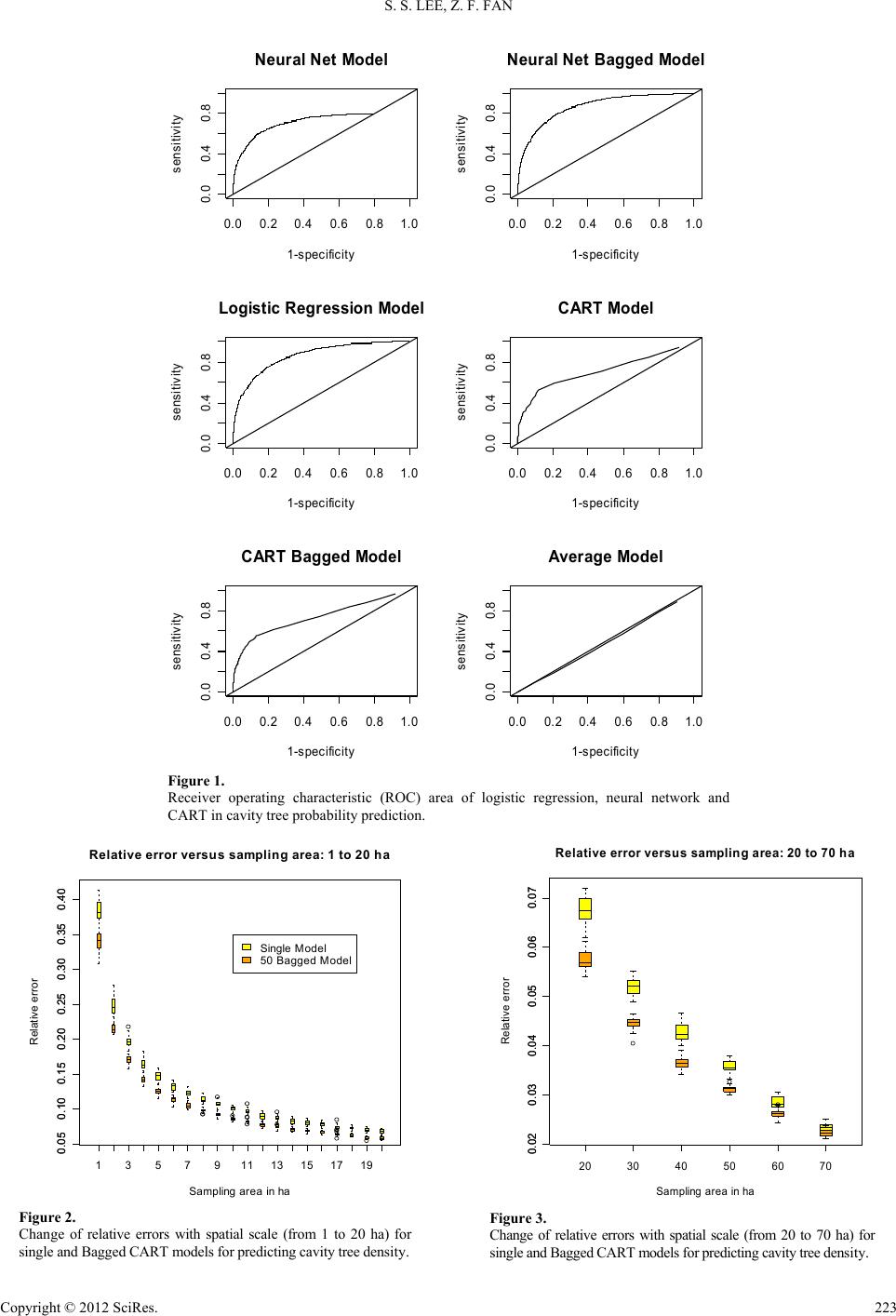
0.021 0.022 0.023 0.024 0.025
0.021 0.022 0.023 0.024 0.025
Sampling Area is 70 ha
50 Bagged Model Relative Error
Single Mo del Relative Erro r
t test p-value < 10^-9
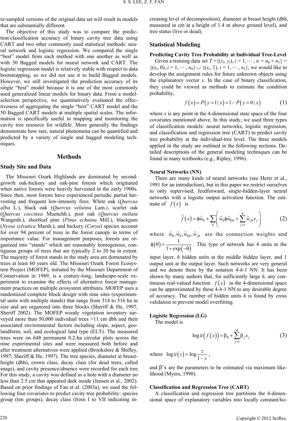
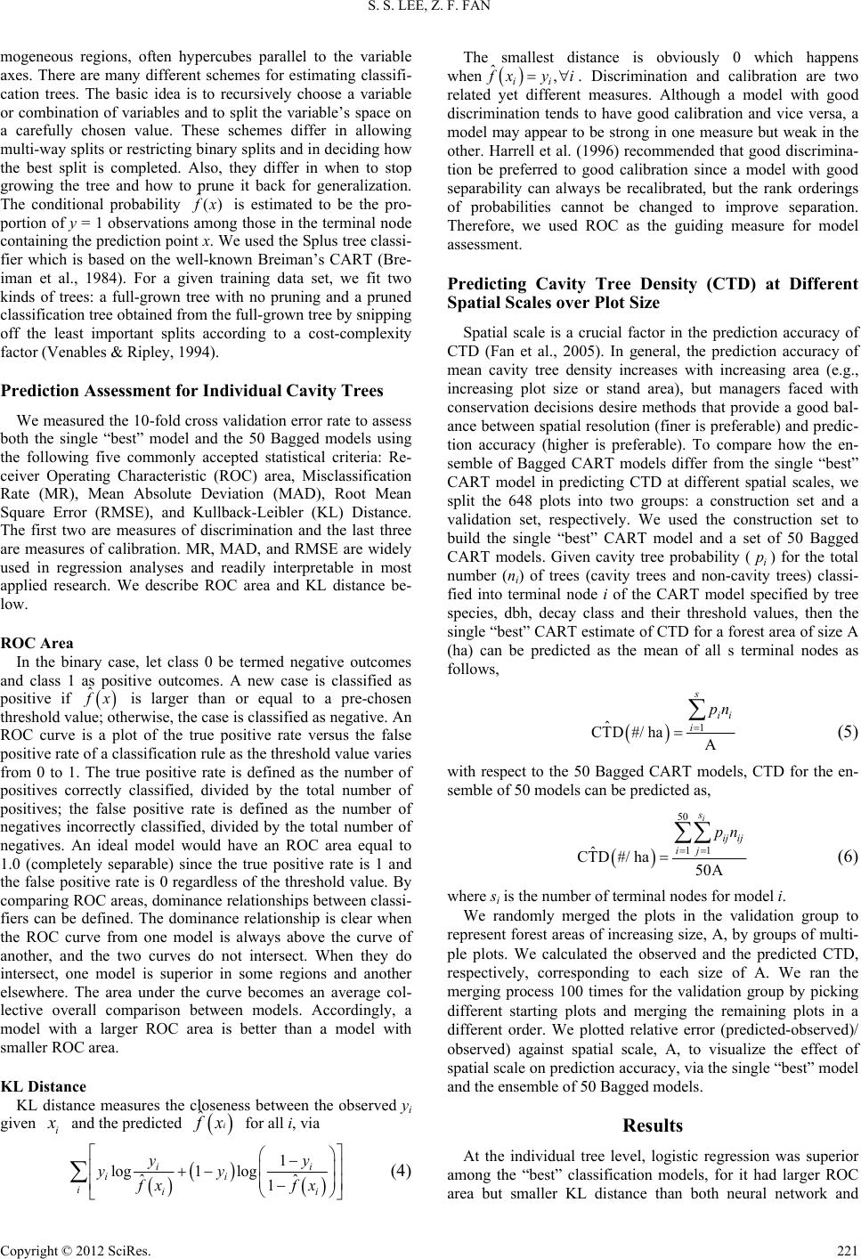
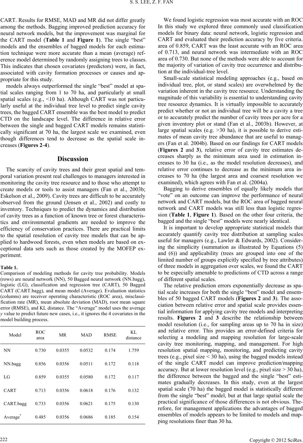
Figure 4.
Scatter plot of relative errors of single and 50 Bagged models at a
spatial scale of 70 ha.
Conclusion
This study constructs three classes of tree-level models to es-
timate probabilities of cavity presence: logistic regression, neu-
ral networks, and CART. The estimated probabilities are com-
bined with known tree counts within covariate classes to predict
mean cavity tree density at different spatial scales, with or
without bootstrap aggregation (bagging). Although logistic
regression was the best model to predict cavity probabilities at
the individual tree level, the bagged CART outperformed other
models in predicting mean cavity tree density at the landscape
scale (e.g., >10 ha). Prediction accuracy, measured in terms of
relative error continues to decrease with spatial scale and the
difference between the bagged CART ensemble and single
CART model remains significant statistically at largest spatial
scale (70 ha) tested in the study. This is largely due to the
non-stationary nature of CART. In addition, the tree profile and
explicit deposition of important covariates in a one-after-an-
other manner of CART make it more useful for landscape level
cavity tree mapping.
Acknowledgements
Mr. Randy Jensen from Missouri Department of Conserva-
tion provided cavity tree data used for these analyses. Dr.
Stephen R. Shifley from USDA Forest Service Northern Re-
search Station reviewed the first draft of this paper. Dr. Michael
K. Crosby from the Department of Forestry, Mississippi State
University helped formatting and reviewing the revised version
of this paper. We thank them all.
REFERENCES
Breiman, L. (1995). Stacked regressions. Machine L e a rn i ng , 24, 49-64.
doi:10.1007/BF00117832
Breiman, L. (1996). Bagging predictors. Machine Learning, 26, 123-
140. doi:10.1007/BF00058655
Breiman, L., Friedman, J. H., Olshen, R. A., & Stone, C. J. (1984).
Classification and regression trees. Monterey, CA: Wadsworth and
Brooks.
Brookshire, B. L., & Shifley, S. R. (Eds.) (1997). Proceedings of the
missouri ozark forest ecosystem project symposium: An experimental
approach to landscape research, St. Louis, 3-5 June 1997.
Carey, A. B. (1983). Cavities in trees in hardwood forests. Snag habitat
management symposium. General Technical Report GTR-RM-99,
US Department of Agriculture Forest Service, 167-184.
Eskelson, B. N., Temesgen, H., & Barrett, T. M. (2009). Estimating ca-
vity tree and snag abundance using negative binomial regression
models and nearest neighbor imputation methods. Canadian Journal
of Forest Research, 39, 1749-1765. doi:10.1139/X09-086
Fan, Z., Larsen, D. R., Shifley, S. R., & Thompson III, F. R. (2003a).
Estimating cavity tree abundance by stand age and basal area, Mis-
souri, USA. Forest Ecolog y an d Ma nagement, 179, 231-242.
doi:10.1016/S0378-1127(02)00522-4
Fan, Z., Lee, S., Shifley, S. R., Thompson III, F. R., & Larsen, D. R.
(2004a). Simulating the effect of landscape size and age structure on
cavity tree density using resampling technique. Forest Science, 50,
603-609.
Fan, Z., Shifley, S. R., Spetich, M. A., Thompson III, F. R., & Larsen,
D. R. (2003b). Distribution of cavity trees in Midwestern old-growth
and second-growth forests. Canadian Journal of Forest Research, 33,
1481-1494. doi:10.1139/x03-068
Fan, Z., Shifley, S. R., Spetich, M. A., Thompson III, F. R., & Larsen,
D. R. (2005). Abundance and size distribution of cavity trees in sec-
ond-growth and old-growth central hardwood forests. Northern
Journal of Applied Forestry, 22,162-169.
Fan, Z., Shifley, S. R., Thompson III, F. R., & Larsen, D. R. (2004b).
Simulated cavity tree dynamics under alternative timber harvest re-
gimes. Forest Ecology and Management, 19 3, 399-412.
doi:10.1016/j.foreco.2004.02.008
Hand, D. J. (1997). Construction and assessment of classification rules.
New York, NY: Wiley.
Harrell Jr., F. E., Lee, K. L., & Mark, D. B. (1996). Multivariable prog-
nostic models: Issue in developing models, evaluating assumptions
and adequacy, and measuring and reducing errors. Statistics in Medi-
cine, 15, 361-387.
doi:10.1002/(SICI)1097-0258(19960229)15:4<361::AID-SIM168>3.
0.CO;2-4
Hertz, J. A., Krogh, A. S., & Palmer, R. G. (1991). Introduction to the
theory of neural computation. Redwood City, CA: Addison-Wesley.
Jensen, R. G., Kabrick J. M., & Zenner, E. K. (2002). Tree cavity esti-
mation and verification in the Missouri Ozarks. General Technical
Report GTR-NC-1227, US Department of Agriculture Forest Service,
114-129.
Johnson, R. A., & Wichern, D. W. (1992). Applied Multivariate Statis-
tical Analysis. Upper Saddle River, NJ: Prentice Hall.
Lawler, J. J., & Edwards, T. C. (2002). Landscape patterns as predictors
of nesting habitat: Building and testing models for four species of
cavity-nesting birds in the Uinta Mountains of Utah, USA. Land-
scape Ecology, 17, 233-245. doi:10.1023/A:1020219914926
McClelland, B. R., & Frissell, S. S. (1975). Identifying forest snags
useful for hole-nesting birds. Journal of Forestry, 73, 414-417.
Myers, R. H. (1990). Classical and Modern Regression with Applica-
tions. Boston: PWS Publishing Company.
Ripley, B. D. (1996). Pattern recognition and neural networks. Cam-
bridge: Cambridge University Press.
Sheriff, S. L. (2002). Missouri ozark forest ecosystem project: The ex-
periment. General Technical Report GTR-NC-227, US Department
of Agriculture Forest Service, 1-25.
Sheriff, S. L., & He, Z. (1997). The experimental design of the Missouri
Ozark Forest Ecosystem Project. General Technical Report GTR-
NC-193, US Department of Agriculture Forest Service, 26-40.
Titus, R. (1983). Management of snags and cavity trees in Missouri—A
process. Snag habitat management symposium. General Technical
Report GTR-RM-99, US Department of Agriculture Forest Service,
51-59.
Venables, W. N., & Ripley B. D. (1994). Modern applied statistics with
S-plus. New York: Springer-Verlag.
Wolpert, D. (1992). Stacked generalization. Neural Networks, 5, 241-
259. doi:10.1016/S0893-6080(05)80023-1
224