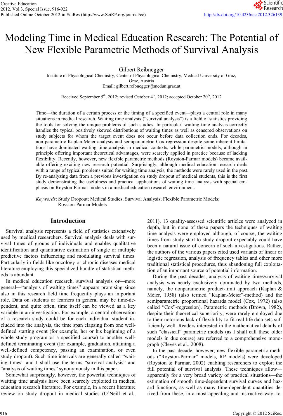
Creative Education
2012. Vol.3, Special Issue, 916-922
Published Online October 2012 in SciRes (http://www.SciRP.org/journal/ce) http://dx.doi.org/10.4236/ce.2012.326139
916
Modeling Time in Medical Education Research: The Potential of
New Flexible Parametric Methods of Survival Analysis
Gilbert Reibnegger
Institute of Physiological Chemistry, Center of Physiological Chemistry, Medical University of Graz,
Graz, Austria
Received September 5th, 2012; revised October 4th, 2012; accepted October 20th, 2012
Time—the duration of a certain process or the timing of a specified event—plays a central role in many
situations in medical research. Waiting time analysis (“survival analysis”) is a field of statistics providing
the tools for solving the unique problems of such studies. In particular, waiting time analysis correctly
handles the typical positively skewed distributions of waiting times as well as censored observations on
study subjects for whom the target event does not occur before data collection ends. For decades,
non-parametric Kaplan-Meier analysis and semiparametric Cox regression despite some inherent limita-
tions have dominated waiting time analysis in medical contexts, while parametric models, although in
principle offering important theoretical advantages, were scarcely applied in practice because of lacking
flexibility. Recently, however, new flexible parametric methods (Royston-Parmar models) became avail-
able offering exciting new research potential. Surprisingly, although medical education research deals
with a range of typical problems suited for waiting time analysis, the methods were rarely used in the past.
By re-analyzing data from a previous investigation on study dropout of medical students, this is the first
study demonstrating the usefulness and practical applications of waiting time analysis with special em-
phasis on Royston-Parmar models in a medical education research environment.
Keywords: Study Dropout; Medical Studies; Survival Analysis; Flexible Parametric Models;
Royston-Parmar Models
Introduction
Survival analysis represents a field of statistics extensively
used by medical researchers. Survival analysis deals with sur-
vival times of groups of individuals and enables qualitative
identification and quantitative estimation of single or multiple
predictive factors influencing and modulating survival times.
Particularly in fields like oncology or chronic diseases medical
literature employing this specialized bundle of statistical meth-
ods is abundant.
In medical education research, survival analysis or—more
general—“analysis of waiting times” appears promising since
also in this research field time frequently plays an important
role. Data on students or learners in general may be time-de-
pendent, and quite often, time itself can be viewed as a key
variable in an investigation. For example, a central observation
of a research study could be for each individual student in-
cluded into the analysis, the time span elapsing from one well-
defined starting event (for example, her or his beginning of a
whole study program or a specified course) to another well-
defined terminating event (for example, graduation, attaining a
well-defined competency, passing an examination, or even
study dropout). Such time intervals are generally called “wait-
ing times” and I shall use the terms “survival analysis” and
“analysis of waiting times” synonymously in this paper.
Somewhat surprisingly, however, the powerful techniques of
waiting time analysis have been scarcely exploited in medical
education research literature. For example, in a recent literature
review on study dropout in medical studies (O’Neill et al.,
2011), 13 quality-assessed scientific articles were analyzed in
depth, but in none of these papers the techniques of waiting
time analysis were employed although, of course, the waiting
times from study start to study dropout expectably could have
been a natural issue of concern of such investigations. Rather,
the authors of the various papers cited used variants of linear or
logistic regression, analysis of frequency tables and other more
traditional statistical procedures, thus abandoning full exploita-
tion of an important source of potential information.
During the past decades, analysis of waiting times/survival
analysis was nearly exclusively dominated by two methods,
namely, the nonparametric product-limit approach (Kaplan &
Meier, 1958) (also termed “Kaplan-Meier”-method) and the
semiparametric proportional hazards model (Cox, 1972) (also
called “Cox”-regression). Parametric methods (Brown, 1982),
despite their theoretical superiority, were rarely employed due
to their notorious lack of flexibility to fit real life data sets suf-
ficiently well. Readers interested in the mathematical details of
such “classical” parametric models (as I shall call these older
models in due course) are referred to a comprehensive mono-
graph (Cleves et al., 2008).
In the past decade, however, new flexible parametric meth-
ods (“Royston-Parmar” models, RP models) were developed
(Royston & Parmar, 2002) enabling researchers to exploit the
full potential of survival analysis. These techniques allow—
apparently for a very broad variety of practical situations—the
estimation of smooth time-dependent survival curves and haz-
ard functions, as well as many time-dependent quantities de-
rived from these, in a most appealing and instructive way, to-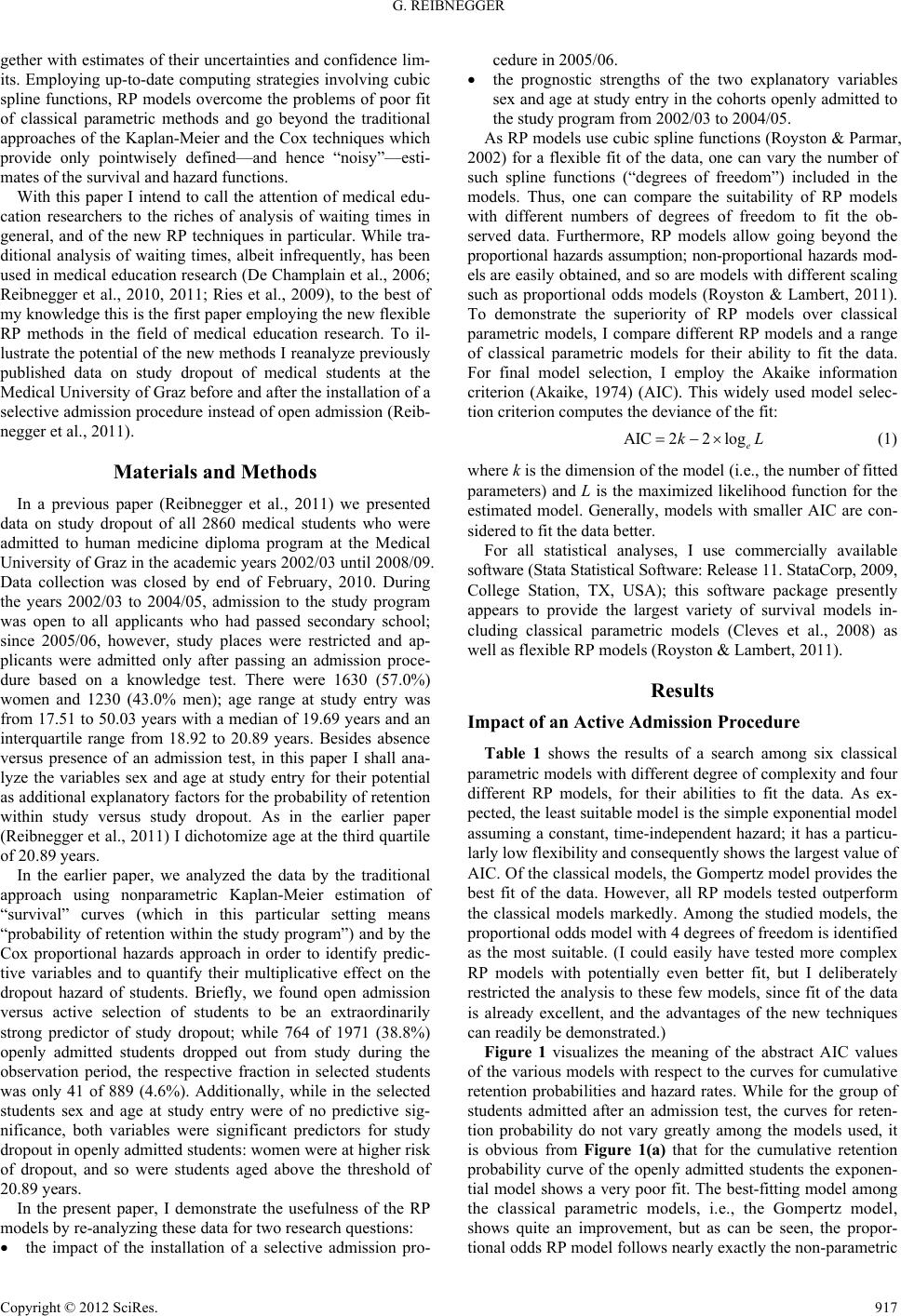

G. REIBNEGGER
gether with estimates of their uncertainties and confidence lim-
its. Employing up-to-date computing strategies involving cubic
spline functions, RP models overcome the problems of poor fit
of classical parametric methods and go beyond the traditional
approaches of the Kaplan-Meier and the Cox techniques which
provide only pointwisely defined—and hence “noisy”—esti-
mates of the survival and hazard functions.
With this paper I intend to call the attention of medical edu-
cation researchers to the riches of analysis of waiting times in
general, and of the new RP techniques in particular. While tra-
ditional analysis of waiting times, albeit infrequently, has been
used in medical education research (De Champlain et al., 2006;
Reibnegger et al., 2010, 2011; Ries et al., 2009), to the best of
my knowledge this is the first paper employing the new flexible
RP methods in the field of medical education research. To il-
lustrate the potential of the new methods I reanalyze previously
published data on study dropout of medical students at the
Medical University of Graz before and after the installation of a
selective admission procedure instead of open admission (Reib-
negger et al., 2011).
Materials and Methods
In a previous paper (Reibnegger et al., 2011) we presented
data on study dropout of all 2860 medical students who were
admitted to human medicine diploma program at the Medical
University of Graz in the academic years 2002/03 until 2008/09.
Data collection was closed by end of February, 2010. During
the years 2002/03 to 2004/05, admission to the study program
was open to all applicants who had passed secondary school;
since 2005/06, however, study places were restricted and ap-
plicants were admitted only after passing an admission proce-
dure based on a knowledge test. There were 1630 (57.0%)
women and 1230 (43.0% men); age range at study entry was
from 17.51 to 50.03 years with a median of 19.69 years and an
interquartile range from 18.92 to 20.89 years. Besides absence
versus presence of an admission test, in this paper I shall ana-
lyze the variables sex and age at study entry for their potential
as additional explanatory factors for the probability of retention
within study versus study dropout. As in the earlier paper
(Reibnegger et al., 2011) I dichotomize age at the third quartile
of 20.89 years.
In the earlier paper, we analyzed the data by the traditional
approach using nonparametric Kaplan-Meier estimation of
“survival” curves (which in this particular setting means
“probability of retention within the study program”) and by the
Cox proportional hazards approach in order to identify predic-
tive variables and to quantify their multiplicative effect on the
dropout hazard of students. Briefly, we found open admission
versus active selection of students to be an extraordinarily
strong predictor of study dropout; while 764 of 1971 (38.8%)
openly admitted students dropped out from study during the
observation period, the respective fraction in selected students
was only 41 of 889 (4.6%). Additionally, while in the selected
students sex and age at study entry were of no predictive sig-
nificance, both variables were significant predictors for study
dropout in openly admitted students: women were at higher risk
of dropout, and so were students aged above the threshold of
20.89 years.
In the present paper, I demonstrate the usefulness of the RP
models by re-analyzing these data for two research questions:
 the impact of the installation of a selective admission pro-
cedure in 2005/06.
 the prognostic strengths of the two explanatory variables
sex and age at study entry in the cohorts openly admitted to
the study program from 2002/03 to 2004/05.
As RP models use cubic spline functions (Royston & Parmar,
2002) for a flexible fit of the data, one can vary the number of
such spline functions (“degrees of freedom”) included in the
models. Thus, one can compare the suitability of RP models
with different numbers of degrees of freedom to fit the ob-
served data. Furthermore, RP models allow going beyond the
proportional hazards assumption; non-proportional hazards mod-
els are easily obtained, and so are models with different scaling
such as proportional odds models (Royston & Lambert, 2011).
To demonstrate the superiority of RP models over classical
parametric models, I compare different RP models and a range
of classical parametric models for their ability to fit the data.
For final model selection, I employ the Akaike information
criterion (Akaike, 1974) (AIC). This widely used model selec-
tion criterion computes the deviance of the fit:
AIC22 loge kL

 (1)
where k is the dimension of the model (i.e., the number of fitted
parameters) and L is the maximized likelihood function for the
estimated model. Generally, models with smaller AIC are con-
sidered to fit the data better.
For all statistical analyses, I use commercially available
software (Stata Statistical Software: Release 11. StataCorp, 2009,
College Station, TX, USA); this software package presently
appears to provide the largest variety of survival models in-
cluding classical parametric models (Cleves et al., 2008) as
well as flexible RP models (Royston & Lambert, 2011).
Results
Impact of an Active Admission Pr oced ure
Table 1 shows the results of a search among six classical
parametric models with different degree of complexity and four
different RP models, for their abilities to fit the data. As ex-
pected, the least suitable model is the simple exponential model
assuming a constant, time-independent hazard; it has a particu-
larly low flexibility and consequently shows the largest value of
AIC. Of the classical models, the Gompertz model provides the
best fit of the data. However, all RP models tested outperform
the classical models markedly. Among the studied models, the
proportional odds model with 4 degrees of freedom is identified
as the most suitable. (I could easily have tested more complex
RP models with potentially even better fit, but I deliberately
restricted the analysis to these few models, since fit of the data
is already excellent, and the advantages of the new techniques
can readily be demonstrated.)
Figure 1 visualizes the meaning of the abstract AIC values
of the various models with respect to the curves for cumulative
retention probabilities and hazard rates. While for the group of
students admitted after an admission test, the curves for reten-
tion probability do not vary greatly among the models used, it
is obvious from Figure 1(a) that for the cumulative retention
probability curve of the openly admitted students the exponen-
tial model shows a very poor fit. The best-fitting model among
the classical parametric models, i.e., the Gompertz model,
shows quite an improvement, but as can be seen, the propor-
tional odds RP model follows nearly exactly the non-parametric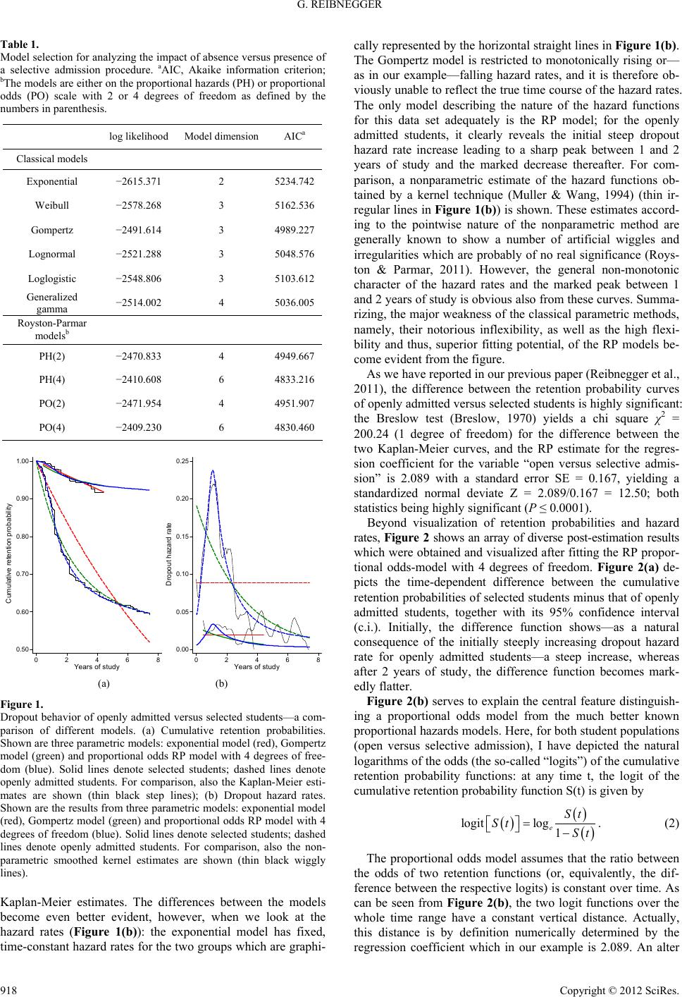

G. REIBNEGGER
Table 1.
Model selection for analyzing the impact of absence versus presence of
a selective admission procedure. aAIC, Akaike information criterion;
bThe models are either on the proportional hazards (PH) or proportional
odds (PO) scale with 2 or 4 degrees of freedom as defined by the
numbers in parenthesis.
log likelihoodModel dimension AICa
Classical models
Exponential −2615.371 2 5234.742
Weibull −2578.268 3 5162.536
Gompertz −2491.614 3 4989.227
Lognormal −2521.288 3 5048.576
Loglogistic −2548.806 3 5103.612
Generalized
gamma −2514.002 4 5036.005
Royston-Parmar
modelsb
PH(2) −2470.833 4 4949.667
PH(4) −2410.608 6 4833.216
PO(2) −2471.954 4 4951.907
PO(4) −2409.230 6 4830.460
0.50
0.60
0.70
0.80
0.90
1.00
Cumulative retention probability
0 2 4 68
Years of study
0.00
0.05
0.10
0.15
0.20
0.25
D r o pout haz ard rate
0 2 4 68
Years of study
(a) (b)
Figure 1.
Dropout behavior of openly admitted versus selected students—a com-
parison of different models. (a) Cumulative retention probabilities.
Shown are three parametric models: exponential model (red), Gompertz
model (green) and proportional odds RP model with 4 degrees of free-
dom (blue). Solid lines denote selected students; dashed lines denote
openly admitted students. For comparison, also the Kaplan-Meier esti-
mates are shown (thin black step lines); (b) Dropout hazard rates.
Shown are the results from three parametric models: exponential model
(red), Gompertz model (green) and proportional odds RP model with 4
degrees of freedom (blue). Solid lines denote selected students; dashed
lines denote openly admitted students. For comparison, also the non-
parametric smoothed kernel estimates are shown (thin black wiggly
lines).
Kaplan-Meier estimates. The differences between the models
become even better evident, however, when we look at the
hazard rates (Figure 1(b)): the exponential model has fixed,
time-constant hazard rates for the two groups which are graphi-
cally represented by the horizontal straight lines in Figure 1(b).
The Gompertz model is restricted to monotonically rising or—
as in our example—falling hazard rates, and it is therefore ob-
viously unable to reflect the true time course of the hazard rates.
The only model describing the nature of the hazard functions
for this data set adequately is the RP model; for the openly
admitted students, it clearly reveals the initial steep dropout
hazard rate increase leading to a sharp peak between 1 and 2
years of study and the marked decrease thereafter. For com-
parison, a nonparametric estimate of the hazard functions ob-
tained by a kernel technique (Muller & Wang, 1994) (thin ir-
regular lines in Figure 1(b)) is shown. These estimates accord-
ing to the pointwise nature of the nonparametric method are
generally known to show a number of artificial wiggles and
irregularities which are probably of no real significance (Roys-
ton & Parmar, 2011). However, the general non-monotonic
character of the hazard rates and the marked peak between 1
and 2 years of study is obvious also from these curves. Summa-
rizing, the major weakness of the classical parametric methods,
namely, their notorious inflexibility, as well as the high flexi-
bility and thus, superior fitting potential, of the RP models be-
come evident from the figure.
As we have reported in our previous paper (Reibnegger et al.,
2011), the difference between the retention probability curves
of openly admitted versus selected students is highly significant:
the Breslow test (Breslow, 1970) yields a chi square χ2 =
200.24 (1 degree of freedom) for the difference between the
two Kaplan-Meier curves, and the RP estimate for the regres-
sion coefficient for the variable “open versus selective admis-
sion” is 2.089 with a standard error SE = 0.167, yielding a
standardized normal deviate Z = 2.089/0.167 = 12.50; both
statistics being highly significant (P ≤ 0.0001).
Beyond visualization of retention probabilities and hazard
rates, Figure 2 shows an array of diverse post-estimation results
which were obtained and visualized after fitting the RP propor-
tional odds-model with 4 degrees of freedom. Figure 2(a) de-
picts the time-dependent difference between the cumulative
retention probabilities of selected students minus that of openly
admitted students, together with its 95% confidence interval
(c.i.). Initially, the difference function shows—as a natural
consequence of the initially steeply increasing dropout hazard
rate for openly admitted students—a steep increase, whereas
after 2 years of study, the difference function becomes mark-
edly flatter.
Figure 2(b) serves to explain the central feature distinguish-
ing a proportional odds model from the much better known
proportional hazards models. Here, for both student populations
(open versus selective admission), I have depicted the natural
logarithms of the odds (the so-called “logits”) of the cumulative
retention probability functions: at any time t, the logit of the
cumulative retention probability function S(t) is given by
 


logitlog 1
e
St
St St 
 . (2)
The proportional odds model assumes that the ratio between
the odds of two retention functions (or, equivalently, the dif-
ference between the respective logits) is constant over time. As
can be seen from Figure 2(b), the two logit functions over the
whole time range have a constant vertical distance. Actually,
this distance is by definition numerically determined by the
regression coefficient which in our example is 2.089. An alter
918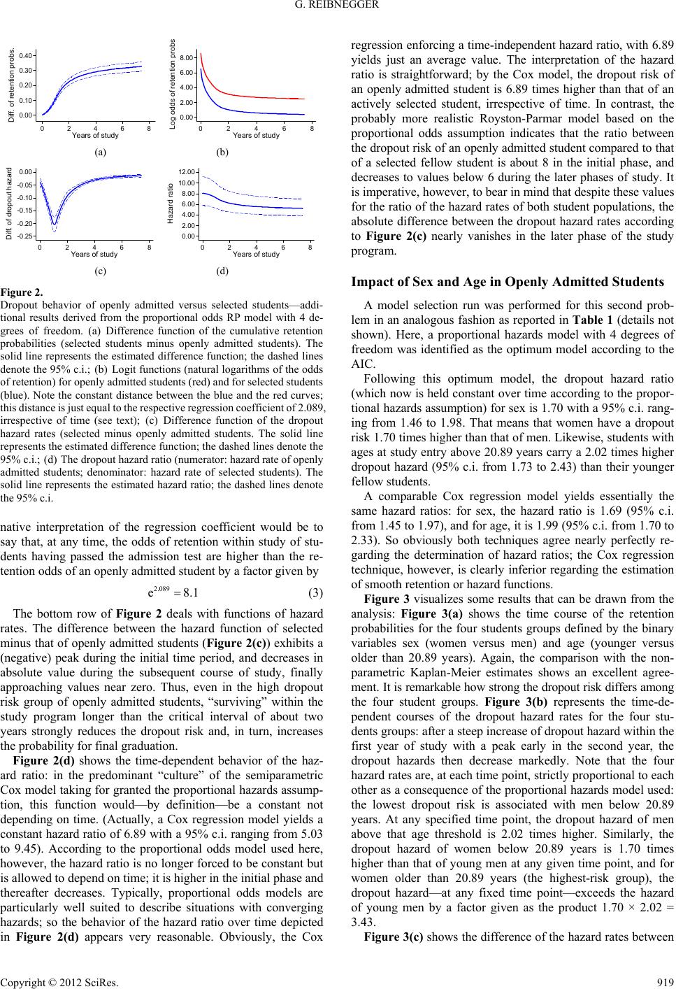

G. REIBNEGGER
0.00
0.10
0.20
0.30
0.40
Di ff. of re t e ntion pro bs .
0 2 46 8
Years of stud y
a
0.00
2.00
4.00
6.00
8.00
Lo g odds of re t ention pr o b s
0 2 4 6 8
Years of stud y
b
(a) (b)
-0.25
-0.20
-0.15
-0.10
-0.05
0.00
Dif f. of d r op out haz ar d
0 24 68
Years of stud y
0.00
2.00
4.00
6.00
8.00
10.00
12.00
Hazard ratio
02468
Years of study
(c) (d)
Figure 2.
Dropout behavior of openly admitted versus selected students—addi-
tional results derived from the proportional odds RP model with 4 de-
grees of freedom. (a) Difference function of the cumulative retention
probabilities (selected students minus openly admitted students). The
solid line represents the estimated difference function; the dashed lines
denote the 95% c.i.; (b) Logit functions (natural logarithms of the odds
of retention) for openly admitted students (red) and for selected students
(blue). Note the constant distance between the blue and the red curves;
this distance is just equal to the respective regression coefficient of 2.089,
irrespective of time (see text); (c) Difference function of the dropout
hazard rates (selected minus openly admitted students. The solid line
represents the estimated difference function; the dashed lines denote the
95% c.i.; (d) The dropout hazard ratio (numerator: hazard rate of openly
admitted students; denominator: hazard rate of selected students). The
solid line represents the estimated hazard ratio; the dashed lines denote
the 95% c.i.
native interpretation of the regression coefficient would be to
say that, at any time, the odds of retention within study of stu-
dents having passed the admission test are higher than the re-
tention odds of an openly admitted student by a factor given by
2.089
e8.1 (3)
The bottom row of Figure 2 deals with functions of hazard
rates. The difference between the hazard function of selected
minus that of openly admitted students (Figure 2(c)) exhibits a
(negative) peak during the initial time period, and decreases in
absolute value during the subsequent course of study, finally
approaching values near zero. Thus, even in the high dropout
risk group of openly admitted students, “surviving” within the
study program longer than the critical interval of about two
years strongly reduces the dropout risk and, in turn, increases
the probability for final graduation.
Figure 2(d) shows the time-dependent behavior of the haz-
ard ratio: in the predominant “culture” of the semiparametric
Cox model taking for granted the proportional hazards assump-
tion, this function would—by definition—be a constant not
depending on time. (Actually, a Cox regression model yields a
constant hazard ratio of 6.89 with a 95% c.i. ranging from 5.03
to 9.45). According to the proportional odds model used here,
however, the hazard ratio is no longer forced to be constant but
is allowed to depend on time; it is higher in the initial phase and
thereafter decreases. Typically, proportional odds models are
particularly well suited to describe situations with converging
hazards; so the behavior of the hazard ratio over time depicted
in Figure 2(d) appears very reasonable. Obviously, the Cox
regression enforcing a time-independent hazard ratio, with 6.89
yields just an average value. The interpretation of the hazard
ratio is straightforward; by the Cox model, the dropout risk of
an openly admitted student is 6.89 times higher than that of an
actively selected student, irrespective of time. In contrast, the
probably more realistic Royston-Parmar model based on the
proportional odds assumption indicates that the ratio between
the dropout risk of an openly admitted student compared to that
of a selected fellow student is about 8 in the initial phase, and
decreases to values below 6 during the later phases of study. It
is imperative, however, to bear in mind that despite these values
for the ratio of the hazard rates of both student populations, the
absolute difference between the dropout hazard rates according
to Figure 2(c) nearly vanishes in the later phase of the study
program.
Impact of Sex and Age in Openly Admitted Students
A model selection run was performed for this second prob-
lem in an analogous fashion as reported in Table 1 (details not
shown). Here, a proportional hazards model with 4 degrees of
freedom was identified as the optimum model according to the
AIC.
Following this optimum model, the dropout hazard ratio
(which now is held constant over time according to the propor-
tional hazards assumption) for sex is 1.70 with a 95% c.i. rang-
ing from 1.46 to 1.98. That means that women have a dropout
risk 1.70 times higher than that of men. Likewise, students with
ages at study entry above 20.89 years carry a 2.02 times higher
dropout hazard (95% c.i. from 1.73 to 2.43) than their younger
fellow students.
A comparable Cox regression model yields essentially the
same hazard ratios: for sex, the hazard ratio is 1.69 (95% c.i.
from 1.45 to 1.97), and for age, it is 1.99 (95% c.i. from 1.70 to
2.33). So obviously both techniques agree nearly perfectly re-
garding the determination of hazard ratios; the Cox regression
technique, however, is clearly inferior regarding the estimation
of smooth retention or hazard functions.
Figure 3 visualizes some results that can be drawn from the
analysis: Figure 3(a) shows the time course of the retention
probabilities for the four students groups defined by the binary
variables sex (women versus men) and age (younger versus
older than 20.89 years). Again, the comparison with the non-
parametric Kaplan-Meier estimates shows an excellent agree-
ment. It is remarkable how strong the dropout risk differs among
the four student groups. Figure 3(b) represents the time-de-
pendent courses of the dropout hazard rates for the four stu-
dents groups: after a steep increase of dropout hazard within the
first year of study with a peak early in the second year, the
dropout hazards then decrease markedly. Note that the four
hazard rates are, at each time point, strictly proportional to each
other as a consequence of the proportional hazards model used:
the lowest dropout risk is associated with men below 20.89
years. At any specified time point, the dropout hazard of men
above that age threshold is 2.02 times higher. Similarly, the
dropout hazard of women below 20.89 years is 1.70 times
higher than that of young men at any given time point, and for
women older than 20.89 years (the highest-risk group), the
dropout hazard—at any fixed time point—exceeds the hazard
of young men by a factor given as the product 1.70 × 2.02 =
3.43.
Figure 3(c) shows the difference of the hazard rates between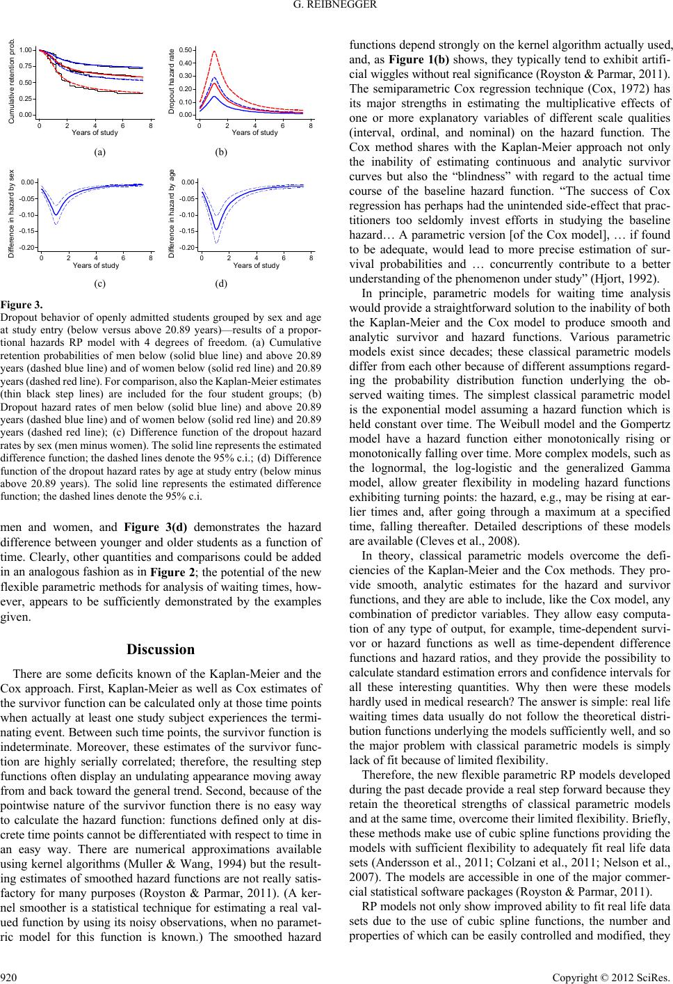

G. REIBNEGGER
0.00
0.25
0.50
0.75
1.00
Cumulative retention prob.
0 2 4 68
Years of study
a
0.00
0.10
0.20
0.30
0.40
0.50
D ropout ha zard rate
0 2 4 68
Years of stud y
b
(a) (b)
-0.20
-0.15
-0.10
-0.05
0.00
Di ffere nce in hazard by sex
0 2 46 8
Years of study
c
-0.20
-0.15
-0.10
-0.05
0.00
Difference in hazard by age
0 2 4 68
Years of stud y
d
(c) (d)
Figure 3.
Dropout behavior of openly admitted students grouped by sex and age
at study entry (below versus above 20.89 years)—results of a propor-
tional hazards RP model with 4 degrees of freedom. (a) Cumulative
retention probabilities of men below (solid blue line) and above 20.89
years (dashed blue line) and of women below (solid red line) and 20.89
years (dashed red line). For comparison, also the Kaplan-Meier estimates
(thin black step lines) are included for the four student groups; (b)
Dropout hazard rates of men below (solid blue line) and above 20.89
years (dashed blue line) and of women below (solid red line) and 20.89
years (dashed red line); (c) Difference function of the dropout hazard
rates by sex (men minus women). The solid line represents the estimated
difference function; the dashed lines denote the 95% c.i.; (d) Difference
function of the dropout hazard rates by age at study entry (below minus
above 20.89 years). The solid line represents the estimated difference
function; the dashed lines denote the 95% c.i.
men and women, and Figure 3(d) demonstrates the hazard
difference between younger and older students as a function of
time. Clearly, other quantities and comparisons could be added
in an analogous fashion as in Figure 2; the potential of the new
flexible parametric methods for analysis of waiting times, how-
ever, appears to be sufficiently demonstrated by the examples
given.
Discussion
There are some deficits known of the Kaplan-Meier and the
Cox approach. First, Kaplan-Meier as well as Cox estimates of
the survivor function can be calculated only at those time points
when actually at least one study subject experiences the termi-
nating event. Between such time points, the survivor function is
indeterminate. Moreover, these estimates of the survivor func-
tion are highly serially correlated; therefore, the resulting step
functions often display an undulating appearance moving away
from and back toward the general trend. Second, because of the
pointwise nature of the survivor function there is no easy way
to calculate the hazard function: functions defined only at dis-
crete time points cannot be differentiated with respect to time in
an easy way. There are numerical approximations available
using kernel algorithms (Muller & Wang, 1994) but the result-
ing estimates of smoothed hazard functions are not really satis-
factory for many purposes (Royston & Parmar, 2011). (A ker-
nel smoother is a statistical technique for estimating a real val-
ued function by using its noisy observations, when no paramet-
ric model for this function is known.) The smoothed hazard
functions depend strongly on the kernel algorithm actually used,
and, as Figure 1(b) shows, they typically tend to exhibit artifi-
cial wiggles without real significance (Royston & Parmar, 2011).
The semiparametric Cox regression technique (Cox, 1972) has
its major strengths in estimating the multiplicative effects of
one or more explanatory variables of different scale qualities
(interval, ordinal, and nominal) on the hazard function. The
Cox method shares with the Kaplan-Meier approach not only
the inability of estimating continuous and analytic survivor
curves but also the “blindness” with regard to the actual time
course of the baseline hazard function. “The success of Cox
regression has perhaps had the unintended side-effect that prac-
titioners too seldomly invest efforts in studying the baseline
hazard… A parametric version [of the Cox model], … if found
to be adequate, would lead to more precise estimation of sur-
vival probabilities and … concurrently contribute to a better
understanding of the phenomenon under study” (Hjort, 1992).
In principle, parametric models for waiting time analysis
would provide a straightforward solution to the inability of both
the Kaplan-Meier and the Cox model to produce smooth and
analytic survivor and hazard functions. Various parametric
models exist since decades; these classical parametric models
differ from each other because of different assumptions regard-
ing the probability distribution function underlying the ob-
served waiting times. The simplest classical parametric model
is the exponential model assuming a hazard function which is
held constant over time. The Weibull model and the Gompertz
model have a hazard function either monotonically rising or
monotonically falling over time. More complex models, such as
the lognormal, the log-logistic and the generalized Gamma
model, allow greater flexibility in modeling hazard functions
exhibiting turning points: the hazard, e.g., may be rising at ear-
lier times and, after going through a maximum at a specified
time, falling thereafter. Detailed descriptions of these models
are available (Cleves et al., 2008).
In theory, classical parametric models overcome the defi-
ciencies of the Kaplan-Meier and the Cox methods. They pro-
vide smooth, analytic estimates for the hazard and survivor
functions, and they are able to include, like the Cox model, any
combination of predictor variables. They allow easy computa-
tion of any type of output, for example, time-dependent survi-
vor or hazard functions as well as time-dependent difference
functions and hazard ratios, and they provide the possibility to
calculate standard estimation errors and confidence intervals for
all these interesting quantities. Why then were these models
hardly used in medical research? The answer is simple: real life
waiting times data usually do not follow the theoretical distri-
bution functions underlying the models sufficiently well, and so
the major problem with classical parametric models is simply
lack of fit because of limited flexibility.
Therefore, the new flexible parametric RP models developed
during the past decade provide a real step forward because they
retain the theoretical strengths of classical parametric models
and at the same time, overcome their limited flexibility. Briefly,
these methods make use of cubic spline functions providing the
models with sufficient flexibility to adequately fit real life data
sets (Andersson et al., 2011; Colzani et al., 2011; Nelson et al.,
2007). The models are accessible in one of the major commer-
cial statistical software packages (Royston & Parmar, 2011).
RP models not only show improved ability to fit real life data
sets due to the use of cubic spline functions, the number and
properties of which can be easily controlled and modified, they
920

G. REIBNEGGER
also go beyond the traditional proportional hazards assumption
(which, as this paper demonstrates, is not necessarily the best
choice) by allowing the user to choose other scales, such as,
e.g., the proportional odds scale or the probit (inverse normal
probability) scale. Clearly, the greatly increased number of
possible modeling options requires methods for model selection;
the Akaike information criterion AIC (Akaike, 1974) is a useful
tool for that purpose. (An alternative to the AIC is the Bayes
information criterion BIC (Schwarz, 1978).)
By re-analyzing published study dropout data before and af-
ter the installation of an admission test for medical students
(Reibnegger et al., 2011) I have addressed two different ques-
tions using RP models. In both cases, I have compared various
RP models with six classical parametric models of increasing
complexity. Model comparison using the AIC shows the
marked improvement of model fit when switching from classi-
cal to RP models. Interestingly, for the first study question,
namely, the impact of the absence versus presence of an admis-
sion test on study dropout, a proportional odds RP model with 4
degrees of freedom was found to fit the data even better than a
comparable proportional hazards model, indicating that the
dropout hazard rates of both student groups converge in the
long run (Bennett, 1983). The graphical comparison of different
models (Figure 1) shows that the simple exponential model is
clearly not suitable to fit the retention probabilities. Among the
other classical parametric models, the Gompertz model was
identified to provide the best fit, and actually its deviation from
the Kaplan-Meier estimates apparently is not very large. How-
ever, the inspection of the hazard rates then provides very con-
vincing evidence that none of the classical models sufficiently
represents the true time dependence of the hazard functions.
The exponential model is restricted to constant hazard rates; it
is, therefore, completely unable to follow the observed course
of the hazard which strongly increases in the early phase, peaks
between year 1 and year 2, and rapidly decreases afterwards.
Also the Gompertz model is not satisfactory; according to its
restriction to monotonically increasing or falling hazard func-
tions, it is unable to reflect the true nature of the hazard func-
tions. In strong contrast, the RP model easily catches the true
course of the hazard functions, while at the same time avoiding
the noisy and wiggly structure of the nonparametric kernel
estimates.
Parametric models adequately fitting the observed data can
be exploited to yield much more detailed information than
nonparametric or semiparametric methods. In contrast to the
latter, differences or ratios between survivor probabilities as
well as between hazard rates of different groups of individuals
are easily obtainable, and so are the confidence intervals of
these quantities. Additionally, many other functions derived
mathematically from the central quantities (cumulative survivor
probability and hazard rate) are accessible, such as, e.g. the
logits (see Figure 2 for examples).
Secondly, the effects of predictor variables sex and age on
cumulative retention probabilities as well as on dropout hazards
were studied in the cohorts of openly admitted students. Again,
I have compared classical as well as RP parametric models for
their suitability to describe these data. Here, a proportional
hazards RP model could be identified as best-fitting model. The
excellent fit of the resulting retention probabilities is obvious
from Figure 3(a). According to the nature of this model, the
hazard functions of the four student groups by sex and age in
this case are strictly proportional, and hazard ratios between
different student groups are therefore constant over time. Nota-
bly, the hazard ratios obtained for the two predictor variables
sex and age are nearly identical to those obtained by a Cox
regression technique. As shown in the Results section, also the
interpretation of these hazard ratios as well as their multiplica-
tive application is identical to the Cox model.
What the Cox model fails to provide, however, is the detailed
time course of the hazard rates and of, e.g., the difference func-
tions between different student groups. The Cox model yields
practically the same information regarding the strengths and the
uncertainties of the constant hazard ratios; it does not, however,
point out clearly enough that the absolute differences between
the hazard functions of men versus women, or of younger ver-
sus older students, after a strong peak in the initial phase of the
study program nearly vanish in the long run. It should be noted
that this important feature is also not easily grasped from Kap-
lan-Meier curves: depicting the cumulative retention (survival)
probabilities, in our example these curves are strongly deter-
mined by the marked initial differences between the hazard
functions. It is mainly within the initial two years that the cu-
mulative plots become separated, and these separations remain
visible despite vanishing differences of hazard rates in the later
years. Thus, the cumulative probability curves visually suggest
a marked difference between the different student groups par-
ticularly at later times; however, as the hazard rates of all
groups nearly vanish at later times, a more appropriate impres-
sion of what really happens is only provided by inspection of
the hazard rates themselves. In conclusion, straightforwardly
drawing the time-dependent differences between the hazard
functions, which is easily accomplished after estimating a RP
model, explicates the intimate details of the time-dependent
hazard rates in a much better way.
An important practical issue for usage of a new statistical
technique by a broad scientific community is the availability of
user-friendly computing software. Kaplan-Meier curves and
Cox models as well as classical parametric models can be ob-
tained by several commercially available software packages
like SAS, STATA and SPSS. Practical examples including the
commands required for performing typical analyses by means
of these mentioned packages are available (Kleinbaum & Klein,
2005). The new flexible RP models can be fitted and analyzed
by STATA Software which to my knowledge presently is the
only commercial package allowing convenient application of
these new techniques. A recent monograph (Royston & Lam-
bert, 2011) presents numerous examples including all the
STATA commands required for even very advanced computa-
tions and for graphical visualization of the results.
Conclusion
The new generation of flexible parametric RP models for
analysis of waiting times opens new horizons to investigate
time-dependent phenomena. The models overcome limitations
of the popular Cox regression method by enabling much more
detailed insight into the time course of hazard rates. Moreover,
being flexible extensions of classical parametric models, they
share the theoretical advantages of the latter while overcoming
their limited applicability due to lack of flexibility. In medical
education research, one could imagine many research questions
that could be studied in greater depth than before by such mod-
els: proper modeling of the time intervals required by students
to attain defined study goals and investigating the detailed in-

G. REIBNEGGER
922
fluences of potential predictor variables by these potent meth-
ods could strongly enhance the spectrum of research directions.
REFERENCES
Akaike, H. (1974). A new look at the statistical model identification.
IEEE Transactions on Automatic Control, 19, 716-723.
doi:10.1109/TAC.1974.1100705
Andersson, T. M. L., Dickman, P. W., Eloranta, S., & Lambert, P. C.
(2011). Estimating and modeling cure in population-based cancer
studies within the framework of flexible parametric survival models.
BMC Medical Research Methodology, 11, 96.
doi:10.1186/1471-2288-11-96
Bennett, S. (1983). Analysis of survival data by the proportional odds
model. Statistics in Medicine, 2, 273-277.
doi:10.1002/sim.4780020223
Breslow, N. (1970). A generalized Kruskal-Wallis test for comparing K
samples subject to unequal patterns of censorship. Biometrika, 57,
579-594. doi:10.1093/biomet/57.3.579
Brown, B. W. Jr. (1982). Estimation in survival analysis: Parametric
models, product-limit and life-table methods. In V. Miké, & K. E.
Stanley (Eds.), Statistics in medical research. Methods and issues,
with applications in cancer research (pp. 317-339). New York, Chi-
chester, Brisbane, Toronto, Singapore: John Wiley and Sons.
Cleves, M., Gutierrez, R., Gould, W., & Marchenko, Y. (2008). An
introduction to survival analysis using stata (2nd ed.). College Sta-
tion, TX: StataCorp LP., Stata Press.
Colzani, E., Liljegren, A., Johansson, A. L. V., Adolfsson, J., Hellborg,
H., Hall, P. F. L., & Czene, K. (2011). Prognosis of patients with
breast cancer: Causes of death and effects of time since diagnosis, age,
and tumor characteristics. Journal of Clinical Oncology, 29, 4014-
4021. doi:10.1200/JCO.2010.32.6462
Cox, D. R. (1972). Regression models and life tables (with discussion).
Journal of the Royal Statistical Society, 34, 187-220.
De Champlain, A., Sample, L., Dillon, G. F., & Boulet, J. R. (2006).
Modeling longitudinal performances on the United States Medical
Licensing Examination and the impact of sociodemographic covari-
ates: An application of survival data analysis. Academic Medicine, 81,
S108-S111. doi:10.1097/00001888-200610001-00027
Hjort, N. L. (1992). On inference in parametric survival data models.
International Statistical Review, 60, 355-387. doi:10.2307/1403683
Kaplan, E. L., & Meier, P. (1958). Nonparametric estimation from in-
complete observations. Journal of the American Statistical Associa-
tion, 53, 457-481. doi:10.1080/01621459.1958.10501452
Kleinbaum, D. G., & Klein, M. (2005). Survival analysis: A self-learn-
ing text (2nd ed.). New York: Springer Science, Business Media,
LLC.
Muller, H.-G., & Wang, J.-L. (1994). Hazard rate estimation under ran-
dom censoring with varying kernels and bandwidths. Biometrics, 50,
61-76. doi:10.2307/2533197
Nelson, C. P., Lambert, P. C., Suire, I. B., & Jones, D. R. (2007). Flexi-
ble parametric models for relative survival, with application in coro-
nary heart disease. Statistics in Medicine, 26, 5486-5498.
doi:10.1002/sim.3064
O’Neill, L. D., Wallstedt, B., Eika, B., & Hartvigsen, J. (2011). Factors
associated with dropout in medical education: A literature review.
Medical Education, 45, 440-454.
doi:10.1111/j.1365-2923.2010.03898.x
Reibnegger, G., Caluba, H.-C., Ithaler, D., Manhal, S., Neges, H. M., &
Smolle, J. (2010). Progress of medical students after open admission
or admission based on knowledge tests. Medical Education, 44, 205-
214. doi:10.1111/j.1365-2923.2009.03576.x
Reibnegger, G., Caluba, H.-C., Ithaler, D., Manhal, S., Neges, H. M., &
Smolle, J. (2011). Dropout rates in medical students at one school
before and after the installation of admission tests in Austria. Aca-
demic Medicine, 86, 1040-1048.
doi:10.1097/ACM.0b013e3182223a1b
Ries, A., Wingard, D., Morgan, C., Farrell, E., Letter, S., & Reznik, V.
(2009). Retention of junior faculty in academic medicine at the Uni-
versity of California, San Diego. Academic Medicine, 84, 37-41.
doi:10.1097/ACM.0b013e3181901174
Royston, P., & Lambert, P. C. (2011). Flexible parametric survival
analysis using stata: Beyond the Cox model. College Station, TX:
StataCorp LP., Stata Press.
Royston, P., & Parmar, M. K. B. (2002). Flexible parametric propor-
tional-hazards and proportional-odds models for censored survival data,
with application to prognostic modelling and estimation of treatment
effects. Statistics in Medicine, 21, 2175-2197. doi:10.1002/sim.1203
Schwarz, G. (1978) Estimating the dimension of a model. Annals of
Statistics, 6, 461-464. doi:10.1214/aos/1176344136