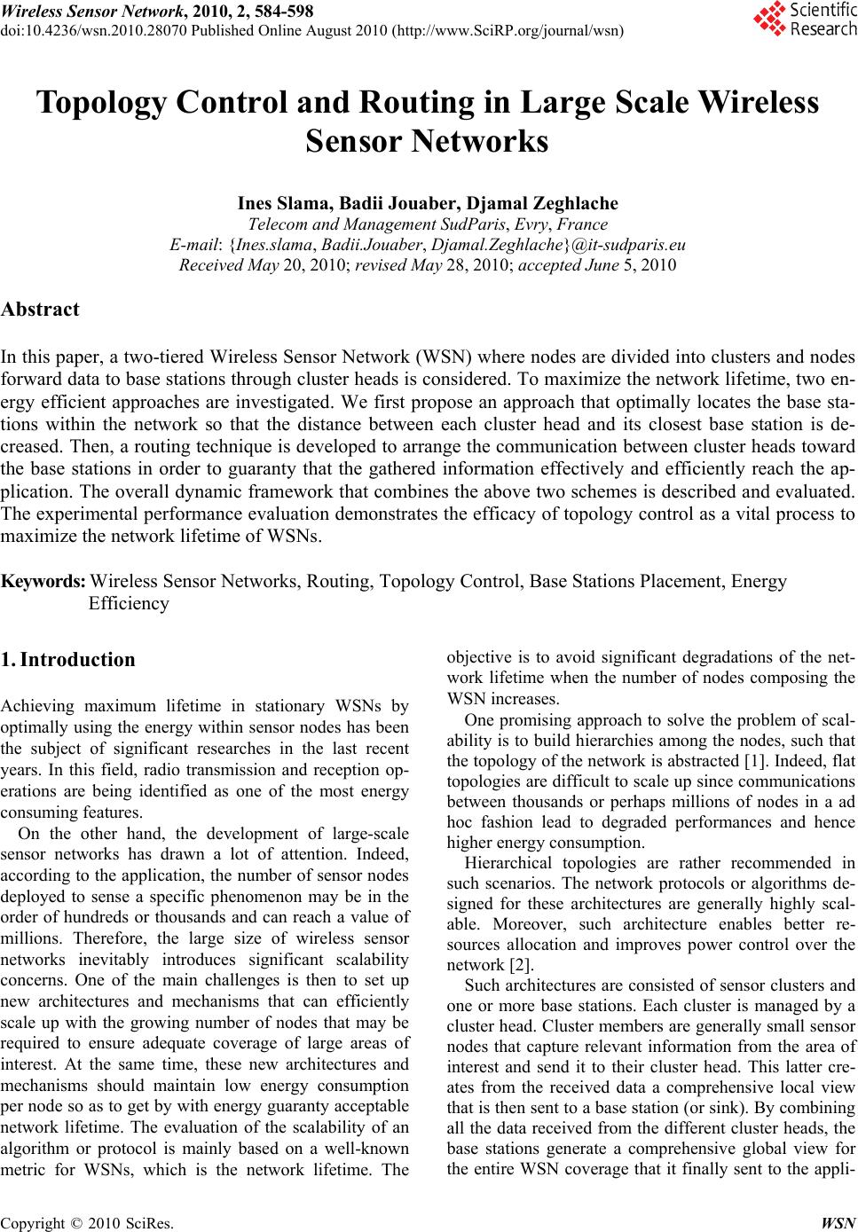Wireless Sensor Network, 2010, 2, 584-598
doi:10.4236/wsn.2010.28070 Published Online August 2010 (http://www.SciRP.org/journal/wsn)
Topology Control and Routing in Large Scale Wireless
Sensor Networks
Ines Slama, Badii Jouaber, Djamal Zeghlache
Telecom and Management SudParis, Evry, France
Received May 20, 2010; revised May 28, 2010; accepted June 5, 2010
Abstract
In this paper, a two-tiered Wireless Sensor Network (WSN) where nodes are divided into clusters and nodes
forward data to base stations through cluster heads is considered. To maximize the network lifetime, two en-
ergy efficient approaches are investigated. We first propose an approach that optimally locates the base sta-
tions within the network so that the distance between each cluster head and its closest base station is de-
creased. Then, a routing technique is developed to arrange the communication between cluster heads toward
the base stations in order to guaranty that the gathered information effectively and efficiently reach the ap-
plication. The overall dynamic framework that combines the above two schemes is described and evaluated.
The experimental performance evaluation demonstrates the efficacy of topology control as a vital process to
maximize the network lifetime of WSNs.
Keywords: Wireless Sensor Networks, Routing, Topology Control, Base Stations Placement, Energy
Efficiency
1. Introduction
Achieving maximum lifetime in stationary WSNs by
optimally using the energy within sensor nodes has been
the subject of significant researches in the last recent
years. In this field, radio transmission and reception op-
erations are being identified as one of the most energy
consuming features.
On the other hand, the development of large-scale
sensor networks has drawn a lot of attention. Indeed,
according to the application, the number of sensor nodes
deployed to sense a specific phenomenon may be in the
order of hundreds or thousands and can reach a value of
millions. Therefore, the large size of wireless sensor
networks inevitably introduces significant scalability
concerns. One of the main challenges is then to set up
new architectures and mechanisms that can efficiently
scale up with the growing number of nodes that may be
required to ensure adequate coverage of large areas of
interest. At the same time, these new architectures and
mechanisms should maintain low energy consumption
per node so as to get by with energy guaranty acceptable
network lifetime. The evaluation of the scalability of an
algorithm or protocol is mainly based on a well-known
metric for WSNs, which is the network lifetime. The
objective is to avoid significant degradations of the net-
work lifetime when the number of nodes composing the
WSN increases.
One promising approach to solve the problem of scal-
ability is to build hierarchies among the nodes, such that
the topology of the network is abstracted [1]. Indeed, flat
topologies are difficult to scale up since communications
between thousands or perhaps millions of nodes in a ad
hoc fashion lead to degraded performances and hence
higher energy consumption.
Hierarchical topologies are rather recommended in
such scenarios. The network protocols or algorithms de-
signed for these architectures are generally highly scal-
able. Moreover, such architecture enables better re-
sources allocation and improves power control over the
network [2].
Such architectures are consisted of sensor clusters and
one or more base stations. Each cluster is managed by a
cluster head. Cluster members are generally small sensor
nodes that capture relevant information from the area of
interest and send it to their cluster head. This latter cre-
ates from the received data a comprehensive local view
that is then sent to a base station (or sink). By combining
all the data received from the different cluster heads, the
base stations generate a comprehensive global view for
the entire WSN coverage that it finally sent to the appli-

I. SLAMA ET AL.585
cation level. In practice, cluster members do not commu-
nicate with each others whereas cluster heads can be in-
volved in inter cluster heads relaying. Both cluster
members and cluster heads are battery powered and en-
ergy constrained. However, cluster heads are considered
to have more computing and storage capacities than
member nodes. Base stations can be mobile or located in
flexible positions and have infinite processing, storage
and power resources. In such scenario, if a sensing node
(cluster member) is drained out of energy, the cluster
head may still be able to provide a comprehensive lo-
cal-view by data generated by other sensor nodes in the
cluster. However, if a cluster head runs out of energy, the
whole cluster coverage is broken. More than that, the
relaying task performed by this cluster head from/to
neighboring cluster heads toward the sink is also lost.
This may affect routes and lead in some cases to the dis-
connection of an entire region of the network, which may
be dramatic for the network mission. Therefore, we are
more concerned about the energy constraint of cluster
heads.
Although cluster heads can have better initial energy
provisioning than sensor nodes, cluster heads also con-
sume energy at a considerably higher rate due to the
transmission of gathered data over much longer distances
[3]. Moreover, cluster heads relay not only data gener-
ated within their own clusters but also data they may
receive from their cluster head neighbors. Cluster Heads
also consume considerable energy for managing their
clusters and gathering information from their cluster
members (reception operations, data aggregation, sig-
naling, etc). Cluster heads perform then two high energy
cost roles. The first is related to forwarding and relaying
tasks and the second concerns their own cluster man-
agement. To increase the network lifetime, the commu-
nication between the cluster heads should be managed in
an energy efficient manner. To this end, an energy aware
routing scheme should be investigated to fairly balance
the energy consumption among the cluster heads ac-
cording to both their available amount of energy and
their role in the network and then route around cluster
heads that are dying or need higher energy to manage
their clusters.
On the other hand, base stations have infinite process-
ing, storage and power resources. Therefore, an efficient
usage of these flexible and mobile base stations to in-
crease the network lifetime should be investigated espe-
cially when the sensing nodes and cluster heads are sta-
tionary or have very low mobility. The idea behind this is
to decrease the distance between each cluster head and
the nearest base station. In fact, when a higher number of
base stations are distributed within the WSN, the paths
length from any cluster head to its nearest base station is
decreased leading to lower energy consumption and
therefore to higher network lifetime. Moreover, since
multi hop communication is used between cluster heads,
the ones that are one hop from the base station drain their
energy faster than other nodes because they have to relay
messages originated from many other nodes (Cluster
Heads) in addition to delivering their own messages.
Therefore, using mobile base stations may help distrib-
uting the energy consumption over the different relaying
cluster heads and then increase the network lifetime.
Base stations trajectories can be rather controlled by the
application or follow a specific mobility model in which
case an estimation of their locations can be computed
like in [4].
Motivated by these issues, we focus, in this paper, on
first, how to optimally locate the base stations in the
network and second, on how to arrange the communica-
tion between cluster heads toward the base stations, both
in order to guaranty that the gathered information effec-
tively and efficiently reach the application. This is gen-
erally referred to as topology control. Our goal is to
maximize the lifetime of a large-scale and energy con-
strained WSN.
The remainder of this paper is organized as follows. A
related work is presented in Section 2. In Section 3, we
give the system architecture of a two-tiered WSN, its
Cluster Heads energy dissipation model, and the defini-
tion of the whole network lifetime. In Section 4, we pre-
sent the approach that optimally locates multiple mobile
base stations in the network such that the energy con-
sumption is fairly distributed over the different Cluster
Heads. In Section 5, by extending an optimal routing
approach presented in a previous work [5], we introduce
a new optimization scheme that arranges the multi-hop
communication between the Cluster Heads while con-
sidering their residual amount of energy and the role they
play in the network leading to a maximum network life-
time. This new optimal routing scheme takes into ac-
count the energy required by each Cluster Head to gather
data from its cluster as well as to relay the packets com-
ing from its Cluster Head neighbors toward the corre-
sponding base station. We describe then in section 6 the
overall dynamic framework. Simulations conducted to
evaluate this global approach are described and com-
mented in section 7. Section 8 concludes this paper and
points out the directions for future work.
2. Prior Work
To solve energy constrained problem in wireless sensor
networks field, many routing protocols have been pro-
posed; especially, cluster based routing protocols have
many advantages such as reducing control messages,
maximizing bandwidth reusability, enhanced resource
allocation, larger scalability and improved power control.
LEACH (Low-Energy Adaptive Clustering Hierarchy)
proposed in [6] includes a distributed cluster formation
technique that enables self-organization of large numbers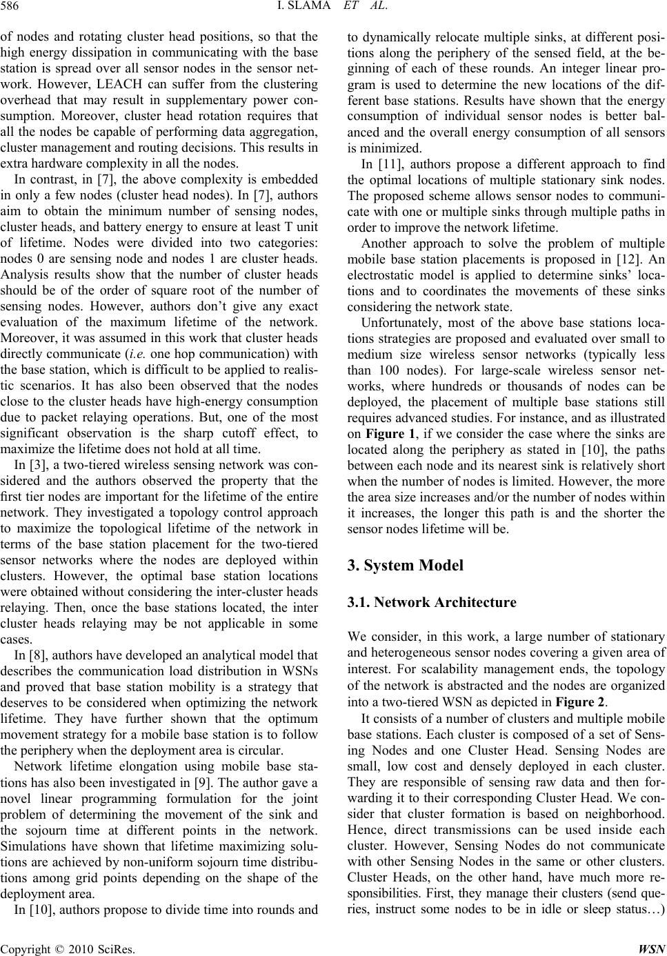

I. SLAMA ET AL. 586
of nodes and rotating cluster head positions, so that the
high energy dissipation in communicating with the base
station is spread over all sensor nodes in the sensor net-
work. However, LEACH can suffer from the clustering
overhead that may result in supplementary power con-
sumption. Moreover, cluster head rotation requires that
all the nodes be capable of performing data aggregation,
cluster management and routing decisions. This results in
extra hardware complexity in all the nodes.
In contrast, in [7], the above complexity is embedded
in only a few nodes (cluster head nodes). In [7], authors
aim to obtain the minimum number of sensing nodes,
cluster heads, and battery energy to ensure at least T unit
of lifetime. Nodes were divided into two categories:
nodes 0 are sensing node and nodes 1 are cluster heads.
Analysis results show that the number of cluster heads
should be of the order of square root of the number of
sensing nodes. However, authors don’t give any exact
evaluation of the maximum lifetime of the network.
Moreover, it was assumed in this work that cluster heads
directly communicate (i.e. one hop communication) with
the base station, which is difficult to be applied to realis-
tic scenarios. It has also been observed that the nodes
close to the cluster heads have high-energy consumption
due to packet relaying operations. But, one of the most
significant observation is the sharp cutoff effect, to
maximize the lifetime does not hold at all time.
In [3], a two-tiered wireless sensing network was con-
sidered and the authors observed the property that the
first tier nodes are important for the lifetime of the entire
network. They investigated a topology control approach
to maximize the topological lifetime of the network in
terms of the base station placement for the two-tiered
sensor networks where the nodes are deployed within
clusters. However, the optimal base station locations
were obtained without considering the inter-cluster heads
relaying. Then, once the base stations located, the inter
cluster heads relaying may be not applicable in some
cases.
In [8], authors have developed an analytical model that
describes the communication load distribution in WSNs
and proved that base station mobility is a strategy that
deserves to be considered when optimizing the network
lifetime. They have further shown that the optimum
movement strategy for a mobile base station is to follow
the periphery when the deployment area is circular.
Network lifetime elongation using mobile base sta-
tions has also been investigated in [9]. The author gave a
novel linear programming formulation for the joint
problem of determining the movement of the sink and
the sojourn time at different points in the network.
Simulations have shown that lifetime maximizing solu-
tions are achieved by non-uniform sojourn time distribu-
tions among grid points depending on the shape of the
deployment area.
In [10], authors propose to divide time into rounds and
to dynamically relocate multiple sinks, at different posi-
tions along the periphery of the sensed field, at the be-
ginning of each of these rounds. An integer linear pro-
gram is used to determine the new locations of the dif-
ferent base stations. Results have shown that the energy
consumption of individual sensor nodes is better bal-
anced and the overall energy consumption of all sensors
is minimized.
In [11], authors propose a different approach to find
the optimal locations of multiple stationary sink nodes.
The proposed scheme allows sensor nodes to communi-
cate with one or multiple sinks through multiple paths in
order to improve the network lifetime.
Another approach to solve the problem of multiple
mobile base station placements is proposed in [12]. An
electrostatic model is applied to determine sinks’ loca-
tions and to coordinates the movements of these sinks
considering the network state.
Unfortunately, most of the above base stations loca-
tions strategies are proposed and evaluated over small to
medium size wireless sensor networks (typically less
than 100 nodes). For large-scale wireless sensor net-
works, where hundreds or thousands of nodes can be
deployed, the placement of multiple base stations still
requires advanced studies. For instance, and as illustrated
on Figure 1, if we consider the case where the sinks are
located along the periphery as stated in [10], the paths
between each node and its nearest sink is relatively short
when the number of nodes is limited. However, the more
the area size increases and/or the number of nodes within
it increases, the longer this path is and the shorter the
sensor nodes lifetime will be.
3. System Model
3.1. Network Architecture
We consider, in this work, a large number of stationary
and heterogeneous sensor nodes covering a given area of
interest. For scalability management ends, the topology
of the network is abstracted and the nodes are organized
into a two-tiered WSN as depicted in Figure 2.
It consists of a number of clusters and multiple mobile
base stations. Each cluster is composed of a set of Sens-
ing Nodes and one Cluster Head. Sensing Nodes are
small, low cost and densely deployed in each cluster.
They are responsible of sensing raw data and then for-
warding it to their corresponding Cluster Head. We con-
sider that cluster formation is based on neighborhood.
Hence, direct transmissions can be used inside each
cluster. However, Sensing Nodes do not communicate
with other Sensing Nodes in the same or other clusters.
Cluster Heads, on the other hand, have much more re-
sponsibilities. First, they manage their clusters (send que-
ries, instruct some nodes to be in idle or sleep status…)

I. SLAMA ET AL.587
(a) (b)
(c)
Figure 1. Multiple base stations placement. (a) a single base
station on the periphery on a small scale WSN; (b) two base
stations on the periphery on a small scale WSN; (c) two
base stations on the periphery on a large scale WSN.
Figure 2. A two-tiered wireless sensor network.
and gather data from their cluster members. Second, they
perform aggregation of this data to eliminate redundancy
and minimize the number of transmissions and thus save
energy. The aggregated data at each Cluster Head repre-
sents a local view of its cluster. Third, they transmit the
composite bit-stream towards the nearest base station.
Each base station can then generate a comprehensive
global view of the entire network coverage by combining
the different local view data received from the different
Cluster Heads [3].
While direct communication is used between Sensing
N
onsibilities can be then defined
fo
gh, both Sensing Nodes and Cluster Heads are
en
allocation plays an important
ro
present the logical
bri
are deployed,
an
.2. Network Graph
e consider that the network is organized into N Clus-
odes and Cluster Heads, it may be inappropriate be-
tween Cluster Heads and Base Stations. Indeed, distances
between them can be large. In such cases, direct trans-
missions will require high power consumption. In addi-
tion, direct transmissions may be simply impossible
since base stations can be out of the range of some Clus-
ter Heads. Multi-hop communication is then used. Con-
sequently, Cluster Heads can also be involved in inter
Cluster Head relaying.
Two main roles/resp
r Cluster Heads. The first is related to their clusters and
consists of managing their cluster members and gather-
ing information from them. The second is related to for-
warding activities and consists of relaying their own
packets as well as packets they may receive from their
Cluster Head neighbors towards the corresponding Base
Station.
Althou
ergy constrained, Cluster Heads are considered to have
more computing and storage capacities than member
nodes. Base Stations, however, have infinite processing,
storage and power resources. They can be mobile or lo-
cated in flexible positions.
Note that initial energy
le in topology control for WSNs. Attributing different
initial energy levels to the nodes according to their posi-
tion and role in the network can significantly improve the
network lifetime [3]. However, since fixed initial energy
sheme is used in practice (among nodes of the same
category, Cluster Heads or Sensing Nodes), we adopt
this scheme for the rest of this paper.
In such scenario, Cluster Heads re
dge between the two tiers of the network architecture:
the lower-tier Sensing Nodes and their Cluster Heads and
the upper-tier Cluster Heads and Base Stations. They are
then vital for the network mission success. Therefore and
as stated previously, Cluster heads should be given all
our attention in terms of energy efficiency.
Once Cluster Heads and Sensing Nodes
immediate challenge is to optimally locate the Base
Stations such that the network lifetime is maximized.
After Base Stations are located, these latters can compute
the inter-Cluster Heads routing scheme. This scheme
should instruct Cluster Heads to communicate in an en-
ergy efficient manner and fairly distribute the energy
consumption among them to achieve a longer network
lifetime.
3
W
ters with one Cluster Head for each Cluster. In the rest of
this paper, we will note a Cluster i by Ci and its corre-
sponding Cluster Head by CHi, i = 1 to N. All the Sens-
ing Nodes in cluster Ci can communicate directly with

I. SLAMA ET AL. 588
eled as an undirected connected
gr
the Cluster Head CH i.
The network is mod
aph G(H,A) where H is the set of Cluster Heads,

, 1
i
H
CHito N and A the set of all undirected
i j CHi, CHj are two Cluster Heads
of H.
Let
links (CH , CH ) where
L be the set of Cluster Heads neighbors of Cluster
H
.3. Energy Model
this work, we assume the following radio energy
i
ead CHi. Li is composed of all Cluster Heads that can
be reached by CHi using a transmission power equal or
less than a maximum predefined threshold. All links are
assumed to be bidirectional.
3
In
model. Note that elec E and amp

represent the energy
consumed respectively to run the radio electronics and
the power amplifier.
Thus, the energy consumed at node when transmit-
tin
i
ij
g information to node j at rate
x
can be written
as:
2
(, )()
tijijelecampijijij ij
ExdEd xex    (1)
And the energy consumed at node when
in
jreceiving
formation from node i at rate ij
x
:
()
rijelec ijrij
ExExex (2)
Moreover, since data aggregation
fo
(fusion) is per-
rmed within the network, the energy consumed at node
j to aggregate information received from node i at rate
ij
x
can be written as:
()
aijij aij
Exx ex

 (3)
where:
Euclid distance between node and node
n
da
ption of one data
un
dij is theij.
eij is the transmission energy required to transmit oe
ta unit from node i to node j.
er is the energy required for the rece
it.

is constant and called the aggregation energy con-
sum
d to the fusion of one data unit.
.4. Lifetime Definitions
irst, we consider that each cluster in the network dies
ole network
as
n this work the lifetime of the whole
cl
fetime can be
ac
. Base Stations Placement
e propose in this section to enhance Base Station
y Multiple
M
large-scale WSN, an intuitively
ap
ach to split a
la
eory related literature, different approaches
an
.1. Existing Graph Partitioning Techniques
[13], a fast approximate graph-partitioning algorithm
ption coefficient [1].
Ea is the energy require
3
F
when no more reliable information can be delivered from
the cluster members. A Cluster Head whose cluster is
dead, continue performing relaying data from/to neigh-
boring Cluster Heads (i.e., its second role).
Second, we define the lifetime of the wh
the metric for determining the optimality of the rout-
ing algorithm.
We define i
uster-based sensor network as the period of time that
ends when a first Cluster Head runs out of energy. This
implies that every Cluster Head is vital for the applica-
tion and cannot be substituted by others.
Hence, maximizing the network li
hieved by delaying as much as possible the first Clus-
ter Head death.
4
W
placement in a two-tiered large-scale WSN.
The idea behind this is to efficiently deplo
obile Base Stations within the network. Multiple Base
Stations are used to decrease the distance between each
Cluster Head and its nearest base station. Base stations
are also chosen to be mobile to make the set of Cluster
Heads close to the Base Stations and then overloaded,
change over the time. This should guaranty a fair distri-
bution of the energy consumption among the different
Cluster Heads in the network and hence improve the
network lifetime. The challenge here is then to define the
initial locations and the movement trajectories of the
different Base Stations.
Since we deal with a
propriate solution is to decompose the underlying
sensor network and then optimize energy usage in each
of the sub-networks independently. The objective is to
take advantage of the powerful and efficient Base Station
placement techniques proposed for small scale WSNs. In
order to apply these techniques over large-scale WSNs,
we propose to first divide the network into sub-networks
according to specific criteria. An adequate Base Station
placement technique can then be applied independently
within each of the defined sub-networks.
Graph partitioning is a promising appro
rge sensor network into balanced sub-networks. In
practice, different criteria can be considered in order to
partition a large-scale two-tiered wireless sensor network.
Since multi-hop communication is used between Cluster
Heads toward base stations, one simple objective is to
create balanced sub-networks (in terms of number of
Cluster Heads/clusters) that group the Cluster Heads ac-
cording to their neighborhood. This allows creating
smaller two-tiered sub-networks with similar characteris-
tics that can be easily optimized, independently but in the
same way.
In graph th
d techniques are proposed for balanced graph parti-
tioning.
4
In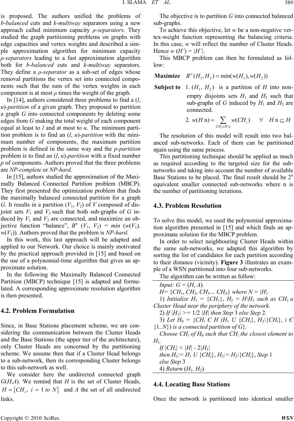

I. SLAMA ET AL.589
l,
u)
proximation of the Maxi-
m
and
ap
he Maximally Balanced Connected
Pa
.2. Problem Formulation
ince, in Base Stations placement scheme, we are con-
rected connected graph
G
is proposed. The authors unified the problems of
b-balanced cuts and k-multiway separators using a new
approach called minimum capacity ρ-separators. They
studied the graph partitioning problems on graphs with
edge capacities and vertex weights and described a sim-
ple approximation algorithm for minimum capacity
ρ-separators leading to a fast approximation algorithm
both for b-balanced cuts and k-multiway separators.
They define a ρ-separator as a sub-set of edges whose
removal partitions the vertex set into connected compo-
nents such that the sum of the vertex weights in each
component is at most ρ times the weight of the graph.
In [14], authors considered three problems to find a (
-partition of a given graph. They proposed to partition
a graph G into connected components by deleting some
edges from G making the total weight of each component
equal at least to l and at most to u. The minimum parti-
tion problem is to find an (l, u)-partition with the mini-
mum number of components, the maximum partition
problem is defined in the same way and the p-partition
problem is to find an (l, u)-partition with a fixed number
p of components. Authors proved that the three problems
are NP-complete or NP-hard.
In [15], authors studied the ap
ally Balanced Connected Partition problem (MBCP).
They first presented the optimization problem that finds
the maximally balanced connected partition for a graph
G. It results in a partition (V1, V2) of V composed of dis-
joint sets V1 and V2 such that both sub-graphs of G in-
duced by V1 and V2 are connected, and maximize an ob-
jective function “balance”, Bw (V1, V
2) = min (w(V1),
w(V2)). Authors proved that the problem is NP-hard.
In this work, this last approach will be adapted
plied to our Network. Our choice is mainly motivated
by the practical approach provided in [15] and based on
the use of a polynomial-time algorithm that gives an ap-
proximate solution.
In the following t
rtition (MBCP) technique [15] is adapted and formu-
lated. A corresponding approximate resolution algorithm
is then presented.
4
S
sidering the communication between the Cluster Heads
and the Base Stations (the upper tier of the architecture),
only Cluster Heads are concerned by the partitioning
scheme. We assume then that if a Cluster Head belongs
to a sub-network, then its corresponding Cluster belongs
to this sub-network as well.
We consider here the undi
(H,A). We remind that H is the set of Cluster Heads,

, 1
i
H
CHito N and A the set of all undirected
rtition G into connected balanced
sub-gra
links.
The objective is to pa
phs.
To achieve this objective, let w be a non-negative ver-
tex-weight function representing the balancing criteria.
In this case, w will reflect the number of Cluster Heads.
Hence w (H’) = |H’|.
This MBCP problem can then be formulated as fol-
low:
121 2
(,)min((),())
w
BHHwH wHaximize M
12
1. (, )
H
HSubject to is a partition of H into non-
empty disjoints sets H1 and H2uch that
sub-graphs
s
of G induced by H1 and H2 are
connected.
( n)()n
i
wHwCHH H
n
2.
i
CH H 

The resolu
anced sub-net
tion of this model will result into two bal-
works. Each of them can be partitioned
ag
the polynomial approxima-
15] and which finds an ap-
ain using the same process.
This partitioning technique should be applied as much
as required according to the targeted size for the sub-
networks and taking into account the number of available
Base Stations to be placed. The final result should be 2n
equivalent smaller connected sub-networks where n is
the number of partitioning iterations.
4.3. Problem Resolution
To solve this model, we used
tion algorithm presented in [
proximate solution for the MBCP problem.
In order to select neighbouring Cluster Heads within
the same sub-networks, we adapted this algorithm by
sorting the list of candidates for each partition according
to their distance (vicinity). Figure 3 illustrates an exam-
ple of a WSN partitioned into four sub-networks.
The algorithm can be written as follow:
Input: G = (H, A).
H= {CH1, CH2, CH3… CHN} where N =
CH }, H = H\H s
|H|.
1) Initialize H1 = {121 uch as CH
1 a
Cluster Head near the periphery of the network.
2) If |H1| >= 1/2 |H| then Step 3 else Step 2.
3) Let H0 = {CHi Є H (H1 U {CHi}, H
2\{CHi}, i Є
{1 a connected ..N}) is partition of G}.
Choose CHi of H0 such that CHi the closest element to
H1.
If |CHi| < |H| - 2|H1|
then H1:= H1 U {CHi}, H2:= H2\{CHi}, Step 1
else Step 3
4) Return (H1, H2).
4.
Once the network is partitioned into identical smaller
4. Locating Base Stations

I. SLAMA ET AL. 590
Figure 3. A Wireless Sensor Network partitioned into 4
sub-networks (the four node patterns represent four dif-
ferent sub-networks).
b-network as centre and the distance between this cen-
nt area is circular.
hen each Base Station
ke
ime, the base station moves
in
this work that each Base Station moves in a
slo
, the base station will more fre-
qu
e the cluster heads will con-
tin
Cluster Heads to efficiently forward the data to
th
Cluster
y first.
ence, to further extend the network lifetime, it is nec-
two-tiered sub-networks, each of these sub-networks is
represented by a disc with the geographic centre of the
su
tre and the farthest Cluster Head (belonging to this sub-
network) from it as radius. Recall that if a Cluster Head
belongs to a sub-network, then its Cluster members be-
long to this sub-network as well.
Base Stations can now be optimally located within
each of these sub-networks independently but in the
same way.
It has been proven in [8] that the optimum movement
for a mobile base station is to follow the periphery when
the deployme
Motivated by this result, we suggest in this work that
one single Base Station be randomly deployed on the
periphery of each sub-network. T
eps moving along the periphery of the sub-network in
which it was deployed. Note that Cluster Heads can send
their data only to the Base Station deployed in the
sub-network they belong to.
A mobile base station can move in two different re-
gimes, a fast mobility regime and a slow mobility regime
[16]. In the fast mobility reg
a continuous form with a velocity v along the time
without any stop or pause in a particular position. In the
slow mobility regime, the base station moves in a dis-
crete form and its trajectory is a sequence of anchor
points between which the base station moves with a ve-
locity v and at which it pauses during a period of time
(epoch).
The slow mobility regime is considered more realistic
and is adopted in many research studies. Therefore, we
assume in
w mobility regime. We propose then to divide time
into rounds. Each Base Station moves then at the begin-
ning of each round and remains at its new position until
the end of the round.
It is very important to carefully choose the value of the
base station velocity. In fact, when the mobile base sta-
tion velocity is high
ently change its position and visit more the different
regions over the area of interest during the network life-
time. Therefore, the energy consumption is efficiently
distributed over the cluster heads and the network life-
time is extended. This can be much more efficient in the
particular case where the cluster heads buffer the data
gathered in their clusters and wait until the base station
approaches to deliver it [4] which reduces unnecessarily
packet forwarding actions since cluster heads are sure of
base station arrival before loosing the data (because of
buffer size limitation or packet deadline expiration). Be-
sides, the high speed moving base station produces a
tolerable data delivery delay especially in the case of fast
mobility regime, which can be very important for some
specific applications. However, base station high veloc-
ity can have negative effects. In fact, it can make the
session interval too short to successfully exchange a long
data packet and hence the packet loss rate will increase.
In slow mobility regime, it is preferred that the epoch
(round) be long enough to guaranty long messages ex-
change.
On the other hand, it seems obvious that the mobility
of the base stations will inevitably incur additional over-
head in data exchanges sinc
uously need to be informed of their corresponding
base station location. However, it has been proved in [16]
that when using a slow mobility regime with an epoch
much longer than the base station moving time, the
overhead introduced by the mobility of the base station
became negligible because amortized across a long ep-
och. This reinforces our choice in using a slow mobility
regime.
After determining the Base Stations placement strat-
egy, we can further prolong network lifetime by in-
structing
e destination. Hence, at the beginning of each round
and after it is located in its new position, each Base Sta-
tion has to compute the routing scheme that will manage
in an energy efficient manner the inter Cluster Heads
communication within its corresponding sub-network
4. Inter-Cluster Head Communication
As discussed at the beginning of this paper,
Heads that are in critical positions run out of energ
H
essary to delay as much as possible the first Cluster
Heads death.

I. SLAMA ET AL.591
ting. It dynamically distributes flows pro-
po
or each node
to
a new con-
st
sa
t these indi-
vi
t
th
ns to be deployed in the
tion k by bk, k = 1 to
For small-scale non-clustered WSNs, we proposed in a
previous work [5] an approach that defines an optimal
multi-hop rou
rtionally to the residual energy available at each node
leading to a maximum network lifetime.
The routing scheme is modelled as an optimization
algorithm and is computed at the Base Station. Its resolu-
tion results in a routing matrix that defines f
which of its neighbors it has to send data.
In this section, we propose to extend this approach to
two-tiered WSN architectures. In addition to the residual
energy at each Cluster Heads, we introduce
raint that reflects Cluster Head energy consumption re-
lated to its intra-cluster activities (i.e. the first role of
Cluster Heads). The idea is to alleviate, from relaying ac-
tivities (i.e. the second role of Cluster Heads), Cluster
Heads requiring higher energy for managing their clusters.
On the other hand, inside each cluster, Sensing Nodes
have to provide the information required by the end ap-
plication. They should be organized such that the QoS is
tisfied with minimum cost. Different techniques can be
used to achieve this goal. For instance, sensors can be
autonomous and self organized [6,17]. Another approach
is to use a relative central mechanism (e.g., scheduling
mechanism) that can take the appropriate decisions on
behalf of the Sensing Nodes. For instance, we can con-
sider that within each cluster, one or more Sensing
Nodes may be used at any time to provide data to the
application, but only certain subsets of available sensors
may satisfy channel bandwidth and/or application quality
of service constraints [18]. In this work, we decide to
adapt the scheduling mechanism, initially proposed in
[18] for a flat topological WSNs, to manage communica-
tions inside the clusters. This scheduler determines
which sensor sets should be used and for how long time
so that the lifetime of the cluster is maximized while the
necessary quality of service expected from this cluster is
always maintained at the application. In addition, Sens-
ing Nodes providing redundant information can be
turned off which contributes in energy saving and re-
duces data flows. Used within each cluster and according
to the performance evaluation given in [18], this mecha-
nism optimizes individual clusters lifetimes.
In order to achieve a global routing optimization , the
inter-Cluster Heads communication approach that we
propose should, in addition, take into accoun
dual clusters lifetimes, as the more a cluster lasts, the
more its Cluster Heads requires energy for its manage-
ment (e.g., reception, data processing and fusion, …).
This inter-Cluster Heads communication approach is
modeled within each sub-network as an optimization
problem. It is then processed in a centralized manner a
e Base Station of each sub-network independently but
simultaneously. It takes into account the current status
and topology of the sub-network and results in a routing
matrix that defines the inter-Cluster Heads flows within
this sub-network such that the minimum Cluster Head
lifetime is optimized.
The inter-Cluster Heads communication approach con-
struction and its details are presented in the following
sections.
4.1. Model and Notations
Let’s consider bBase Statio
etwork. We note a Base Sta
N
aph
nb N.
The network gr G is then partitioned into b N equi-
valent sub-graphs. We consider (H1, H
2, …,b
N
H
) the
connected partition of G.
conThen, each sub-network k corresponding to-
tains one single mobile Base Station bk and NClus-
te
Hk
CH
k
r Heads, k = 1 tob N, CH
k
k
NN

.
We assume that each sub-network k is med as a
connected sub-grapGk 1
odel
h (Hk, Ak), k = tHk is then
the set of Cluster Heads belonging to tnetwork k,
Clus
that can be reached by CHk,i. All
lin
note by the
lete set of Sensing Nodes within a
cl
ob N.
e sub-h
Hk = {CHk,i, i = 1 to CH
k
N} and Ak the set of the undi-
rected links (CHk,i, CHk,j) where CHk,i and CHk,j are two
Cluster Heads of Hk.
Let Lk,i be the set of ter Heads neighbors of Clus-
ter Head CHk,i in the sub-network k. Lk,i is composed of
all Cluster Heads of Hk
ks are assumed to be bidirectional.
We remind that if a Cluster Head belongs to a
sub-network than its corresponding Cluster belongs to
this sub-network as well. We will ,ki
Cluster of Sensing Nodes corresponding to the Cluster
Head CHk,i and then belonging to sub-network k, i = 1
to CH
k
N and k = 1 tob N.
Each cluster ,ki
C contains ,
S
ki
N Sensing Nodes. We
will refer to the comp
C
uster ,ki C as



,
,1.,
S
kil ki
Sl N .
We remind that all Sensing Nodes in Cluster ,ki C can
communicate dire
,, .., ki
S
ctly with their Cluster Head CHk,i and
that all Cluster Heads or
ha
re mb
k,i the arrival rate of information at CHk,I
CHk,i belonging to sub-netwk k
ve to forward the gathered data to the Base Station bk
deployed within this same sub-network. Also, Cluster
Heads belonging to one sub-network cannot communicate
with Cluster Heads belonging to another sub-network.
We finally assume that ,
S
kil
E and ,
CH
ki
E are the initial
energies of Sensing Node ,kil S and Cluster Head CHk,I
spectively. In Table 1, we list all syols used in the
rest of this paper.
4.2. Flow Conservation
We denote by r

I. SLAMA ET AL. 592
otations. sensey thd
we dte bfter
aggreg n.
Table 1. N
Symbol Description
N the numsters in the network.ber of Cluster Heads/Clu
H
d be Sensing Nodes within its cluster C
k,i an
enoy ,ki
v the rate of information at CHk,i a
atio
Hence, ,ki v can be written as, ,, ()
kiaki
vfr. a
f
is a
typical linear agegation function such that ()
a
the set of N Cluster HSN. eads of the W
A the set of the undirected links between the Clustegr
f
xx


for some consta
r
Heads of H
CHi a Cluster Head of H.
Ci the Cluster corresponding to CHi.
Li the set of Cluster Head
, 0 <

< 1.

is called the data
nt

ag n ra
n that tran-
t ipoh
ensed by the cluster members and
gr
ceived from
gregatiotio [1].
Let ,ki w be the average rate of informatio
sit through CHk,i. Is comsed of te generated infor-
mation rate at CHk,i (s
th e
s neighbours of CHi.
ed in the network.
C Hk.
k.
CHk,iin
Ck,i CHk,i.
Sk,il
k,i.
rk,i eata at CHk,i.
vk,i d data at CHk,i.
Nb the number of base stations deploy
Hk a partition of H.
bk the base station deployed in sub-graph k.
Hk,i
CH
a Cluster Head of
k
N the number of Cluster Heads in sub-graph
Heads Neighbors of
Lk,i the set of Cluster
sub-graph k.
the cluster in sub-network k corresponding to
,
S
ki
N the number of Sensing nodes in Ck,i.
Sk,i the set of Sensing Nodes in Ck,i.
a Sensing Node of Sk,i.
,l
E
CH
S
ki the initial energy of Sk,il.
,ki
E the initial energy of CH
the arrival rate of sensd d
the arrival rate of aggregate

the data agregation ratio.
fa the aggregation function.
en aggated at CH k,i) plus the information rate re-
its Cluster Heads neighbours of Lk,i.
,ki
w is given by:
,,
,, ,,
/(, {1,...,})
kj ki
CH
kikik jikjk
jCH L
wvpwkiN

 

(4)
and
i,
{1,..., }
CH
kk
bk
iN
wv



(5)
e is the proportion of data transmitte
k,j to CHk,i.
Obviously, ijand
y the routing trix within sub-
ne which can be writte
wher
CH
,,kji kj
pw d by
,0 (,,) kij
pk
k
p

,,
1 (, {1,...,})
CH
ki N .
We denote b
,
/kj kikij jCH L

k
Pma
twork k and n as:


,kkij
Pp 
Note that Equations (4) and (5) verify the flow con-
servation condition. The flow conser
wk,i at transit through CHk,i.
t transit through bk.
Pk
Tkk k.
Tnet le network.
the average rate of data th
k
b
w the average rate of data tha
pk,ij The flow portion transmitted from CHk,i CHk,j.
the routing matrix within sub-network k.
,
CH
C
ki
T the lifetime duration of Ck,i.
,ki
T the lifetime duration of CHk,i.
the lifetime duration of sub-networ
the lifetime duration of the who
Fk,i the set of feasible sensor sets in Ck,i.
Fk,im a feasible sensor set of Fk,i.
,
F
ki
N the number of feasible sensor sets in C
vation condition
states that the sum of information generation rate and the
total incom
-
red from the cluster Sensing
ifetime of a cluster by
first Cluster Head runs out of energy. We analogically
defi
ing flow must equal the total outgoing flow.
4.3. Lifetime Model
e remind that a cluster dies when no more reliable inW
formation can be delive
odes. We denote the lN,ki C
luste
,
C
ki
T.
Once its cluster dead, each Cluster head continue per-
forming relaying activities until it is over of energy. We
then denote by ,
CH
ki
T, the lifetime of Cr Head
,ki
CH .
The lifetime of the whole network is defined, as stated
in Subsection 3.4, as the period of time that ends when a
th
k,i.
,
F
kim
T the length of time that Fk,im is being u
Schedule of Ck,i.
sed in the optimal
qk,il the power consumption at sensor Sk,il.
elec
E the energy consumed to run the radio electronics.
amp

the energy consumed to run the power amplifier.
ek,ij
er nit.
the transmission energy required to transmit one data
unit from CHk,i to CHk,j .
the energy required for the reception of one data u
ea the energy required to the fusion of one data unit.

the aggregation energy consu
nee lifetime of a sub-network k as the period of
time until which the first Cluster Head ,ki CH dies and
denote it by k T. Then, k T can be written as:
min ,
CH
TTk
,
{1,...,}
CH
k
kk i
iN 

 (6)
mption coefficient.

I. SLAMA ET AL. 593
fined
ntthes.
ork le, denothen be
written as follow:
im
4.4. Intra-Cluster Communication
nspired from [18]. The communications in-
de the clusters is managed by an optimized scheduler
be used and for
axi-
in
Thus, the network lifetime can be deas the pe-
riod of time uil which first sub-network die
The netwifetimed by , can t
net
T
,
, {1,...,}
minmin CH
k
CH
netkk i
kkiN
TT T

 (7)
eHence, maximizing the network lifet can be achie-
ved by maximizing each sub-network lifetime simulta-
neously.
As already mentioned, the intra-cluster communication
scheme is i
si
that determines which sensor sets should
ow long time so that the lifetime of the cluster is mh
mized while the necessary quality of service is respected.
As defined in [18], a sensor set is determined to be fea-
sible if 1) the total bandwidth necessary to support the set is
below the capacity of the cluster and the traffic is schedul-
able and 2) the set provides the necessary reliability to the
application. We will refer to the set of feasible sensor sets
a cluster Ck,i as


,, ,
,1,...,
F
kikimki
FFm N .
The optimal scheduler that maximizes the lifetime of
Ck,i determines the length of time that each sensor set in
Ck,i should be used. Let ,
F
kim
T represent the length of
time that feasible sensor set ,kim
F
is being used in the
op
Finally, we define qk,il as a variable that rep
power consumption (sensing and communication) at
se
troduces the following
S
timal schedule of Ck,i. The objective of the problem is
to maximize the lifetime of each cluster Ck,i:
,,
{1,...,}
CF CH
ki kimk
m
TTi N
 (8)
We will define ak,ilm as a variable equal to one if sensor
Sk,il is being used in feasible sensor set Fk,im of the cluster
Ck,i and equal to zero otherwise.
,,, ,,
( ,{1,...,},{1,...,})
FS CH
kilm kim kilkilkki
m
aTqEkiN lN

(9)
This scheduling problem has been modeled as a gener-
alized maximum flow graph problem. The same method
will be used for each cluster in the network and carried
out in a centralized manner by an unconstrained node
or at the application level at the beginning of the network
deployment and once the clusters are formed (during the
set-up phase and before the transmission phase is started).
The computation of this optimization scheme defines for
each cluster the optimal Schedule that maximizes its life-
time. Each Cluster lifetime value can then be computed
and used as an input parameter for the inter-Cluster
Heads communication scheme.
To have details about the resolution of this optimiza-
tion problem the reader is referred to [18].
4.5. Maximizing Network Lifetime
According to the scheduling problem described in the last
section the lifetime of each cluster Ck,i (not including the
corresponding CHk,i) is . During this period of time a
Cluster Head CHk,i is providing two functionalities: the
first concerns internal exchange (receiving and aggregat-
ing data coming from its cluster members) and the second
concerns external exchange (receiving, transmitting and
relaying the data coming from its Cluser Head neighbors).
,
C
ki
T
Once this period achieved, CHk,i, if not yet drained out
of energy, expend its remaining energy to provide only
the second functionality.

,k
resents the
During the period of time, CHk,i expends an
amount of energy given by Equation (10).
,
C
ki
T
Here, is the transmission energy required to
transmit one data unit from CHk,i to CHk,j relatively to
Equation (1).
,kij
e
So, the remaining energy at CHk,i when is spent is:
,
C
ki
T
2
,,
CH CH
CH
kiki ki
EEE
1
,
(11)
nsor Sk,il.
We remind that ,
S
kil
E is the initial energy of Sensor
Node S. This finite energy in
Hence, according to the energy model described in
Subsection 3.3, the lifetime of CHk,i under a given system


,kkij
Pp( ,{1,...,})
CH
k
ki N is given by Equation (12).
k,il
constraint:
1
,,
, ,,,
/
(
kj ki
kikij kijki
jCHL
T epw



,,
, ,,
/
kj ki
CH C
kirk jikjarki
jCHL
E epweer


,
()) (10)
2
,, ,,
,, ,,
,,
,
,,
,,,, ,
//
,,,,,,, ,
)
ki
r
//
,
,,, ,
//
()
(()
kj kikj ki
kj kikj ki
kj ki
CH C
ki kki
kijkijkirk jik j
jCHLjCH L
CH C
kikikijkijkirkjikjar
jCH LjCH L
C
ki
k ijk ijk irkji
jCHjCH L
TPTepw epw
ETepwepw ee
Tepw ep



 

 



CH
ki
E
(12)
,, , kj kikj
Lw 


I. SLAMA ET AL. 594
Then the lifetime of sub-graph k, can be approxi-
mated as follow:
(13)
Maximizing the lifetime of a sub-network k can be
ached by solving the following optimization problem:
The last constraint models energy conservation at each
Cluster Head CHk,i.
The resolution of this system requires determining the
matrix Pk defining, for a fixed position of Base Station bk,
the optimal routing flows that are used by each Cluster
Head within sub-network k to forward data to
Neighbors such that the lifetime of this sub-netwo
m
on at the Base Station b.
ll dynamic frame-
time maximization. The framewo
isation scheme related to both Base Stations position-
communication presented
m is then defined to permit
e dynamic adaptation of the optimization process (see
the periphery of each sub-network. Time is
th
Input: G(H, A).
,k T,
0.1. The network is divided into Nb equivalent sub-networks.
0.2. One mobile base station is deployed on the periphery of each of
,
{1,..., }
()min(),
CH
k
CH
kkkik
iN
TPT Pk

 these sub-networks.
0.3. Initial round duration (epoch) is de
re
,,
,
,
/
{1,..., }/
0 {1,...,}
kj ki
CH
ki
j k
kij k
jCH L
iNandj CHL
piN

 


M
12
,, ,
{1,...,}
CH CH CH CH
kikikik
EE EiN

(14)
,, k jki
CH
0
k
T
p
aximize
Subject to
its
rk is
aximized. The optimal matrix Pk can then be computed
in a centralized fashik
This optimisation problem is Non Polynomial and can
then be solved over Matlab using specific heuristics
similar to those used to solve the optimization problem
presented in [5]. Once the different sub-networks life-
times , 1
kb
TktoN are computed, the whole net-
work lifetime can be finally given by:
min
netk
k
TT (15)
5. Global Framework
In this section we describe the overa
work for large two-tiered wireless sensor networks life-
rk is based on the opti-
m
ing and inter-Cluster Head
reviously. A cyclic algorithp
th
Figure 4).
Once the nodes are deployed in the interested area, the
network topology is first abstracted and the overall net-
work is partitioned into equivalent sub-networks that
have the same characteristics and where the energy con-
sumption can be optimized independently but in the
same way. One mobile base station is then randomly
deployed on
en divided into equal periods of time called rounds or
epochs. At the beginning of each round, each base station
moves along the periphery of its corresponding sub-
network. Once it reached its new position, the base sta-
tion collects information about the current topology
termined at the application
level
While (the sensor network is operational for the application) do
{//begin of the round
{1,..., }
b
kN :
1) Base station bk in sub-network k moves to its new position on the
periphery
2) At base station bk: Collection of all relevant information from all
the cluster heads of Hk concerning the current topology of sub-network
k.
3) At base station bk: Run of the optimization process and compute
the routing matrix [Pk].
4) Base station bk transmits to each Cluster Head CHk,i the vector
[P ]
k,ij
(,,
{1 . . .}/
CH
kkjki
iNandjCHL).
5) Each Cluster Head sends the captured/received information to its
neighbors toward bk according to [Pk].
// end of the round}
Figure 4. Global framework.
a next step, each base station runs the routing opti-
consumption over the different Cluster Hs according
to their roles in the sub-network and to the residual
he collected data is
aggred by the cluster heads toward
e correspondtimized rout-
g probabilities.
.1. Base Stations Placement
partitioning technique on the
status of its sub-network. These information may include
The residual energy at each sensor node, the neighbors list
and the positions of each node, sources’ throughputs, etc.
In
mization process corresponding to its sub-network as
described in the previous section and which results in an
updated routing matrix that optimally distributes energy
ead
amount energy at each of them. Data gathering is then
p sensing nodes and terformed by the
gated and forwarde
th
in
ing base station using the op
6. Simulations
This section is dedicated to the evaluation of the per-
formances of first, the Base Stations Placement scheme
that optimally locates the different base stations in the
network while considering scalability as well as energy
efficiency issues and second, the inter-Cluster Head
communication approach formulated as an optimization
problem that aims to efficiently and fairly distribute the
energy among Cluster Heads while taking into account
their roles in the network.
6
he effect of the proposed T
WSN lifetime is investigated using numerical simula-
tions over Matlab environment. A circular large-scale
wireless sensor network, with a radius R = 500 m is con-

I. SLAMA ET AL.595
ommunication range r = 80m
nd an initial energy of 1000 J unit. Base Stations are
because they have
rechargeable. We
se sta-
tio
s radius.
en run to compare the net-
wthe two different cases of each of the
th
sidered. In order to study the performance of the base
stations placement scheme, we focused on the upper tier
of the network architecture (Base Stations and Cluster
Heads) independently of the lower tier (Cluster Heads
and Sensing Nodes). 1000 nodes (Cluster Heads) are
randomly (uniformly) deployed over a network area. All
nodes are similar with a c
a
assumed to have no energy constraints
rger batteries or their batteries arela
assumed, in this scenario, that the shortest path routing
algorithm is used to establish routes from Cluster Heads
to base stations. The network lifetime is defined as the
moment at which the first node runs out of energy. Time
is divided into rounds. Each round is composed of T =
100 timeframes. Each sensor node generates one data
packet every timeframe.
To evaluate the efficiency of the proposed graph parti-
tioning technique in elongating the network lifetime,
three comparative scenarios are considered:
1) Scenario 1:
Case 1: An entire large network (not partitioned) is
considered. All the sensors have the same capacity. N
base stations are randomly fixed inside the coverage area
of interest. Each sensor has to send the data it senses to
the nearest base station.
Case 2: The graph-partitioning algorithm (detailed in
Subsection 4.3) is used to define N smaller sub-networks.
One single base station is then randomly fixed in each
sub network. Each sensor node sends its data to the base
station deployed inside the sub-network the sensor node
is belonging to.
2) Scenario 2:
Case 1: The entire network is considered. N mobile
baeployed randomly. Then, the base stations are d
ns start to move inside the area of interest following
the random waypoint model [19]. At the beginning of
each round, each base station moves 60 m.
Case 2: N sub-networks are defined using the graph-
partitioning algorithm and one single base station is ran-
domly deployed in each sub network. Then each base
station moves 60 m each round. The base station cannot
go outside the area of the sub-network it belongs to. This
area is represented by a disc with the geographic centre
of the sub-network as centre and the distance between
this centre and the farthest sensor (belonging to this sub-
network) from it a
3) Scenario 3:
Case 1: The entire network is considered. N mobile
base stations are deployed randomly on the periphery of
the network. Then, the base stations start to move along
the periphery. In one round each base station moved 60
m.
Case 2: The graph-partitioning algorithm is used to
define N smaller sub-networks. One single base station is
randomly deployed on the periphery of each sub network.
Then each base station moves 60 m each round on the
periphery.
We consider that the time required by a base station to
move to its next position is negligible compared to a
round duration.
Several simulations are th
ork lifetime in
ree different scenarios.
Simulation results are presented in Figures 5, 6 and 7.
0
248
n
50
100
150
lifetim
200
250
300
350
e duration (rounds)
450
400
umber of sinks
case1
case2
Figure 5. The network lifetime in Scenario 1.
0
100
200
300
400
500
600
700
800
900
1000
248
number of sinks
lifetime duration (rounds)
case1
case2
Figure 6. The network lifetime in Scenario 2.
0
200
400
600
800
1000
1200
248
case1
number of sinks
case2
Figure 7. The network lifetime in Scenario 3.
lifetime duration (rounds)

I. SLAMA ET AL. 596
hey respectively compare the performance of the dif-
ferent base stations deployment strategies in the case of
partitioned and non-partitioned network (Scenario 1, 2
and 3).
First, let’s notice that the simple use of multiple base
stations enhances the network lifetime (with and without
partitioning). Indeed, the network lifetime increases
proportionally to the number of base stations because the
distance between the nodes and their correspondent base
stations is shortened. Second, it can be seen that moving
the base stations clearly prolong the operation of the
network. In fact, figures show that the network lifetime is
much longer when the base stations are moving (Sce-
nario 2 and 3 with or without partitioning) than when
they are fix (Scenario1). This result is valid with or
withou
enhancement is the most significant in the third
sc
ones situated along the peripheries
of
the
sub-network they belong to whereas they are closer to a
ba
ation is
ndomly
of the pro-
po
e scenario where the sizes of the clusters vary
w
we randomly generate feasible
se sets in a
cler heads
is
of
ber of
se
e 9, which illustrates
T
t partitioning.
Third, enhancements of the network lifetime can be
observed in the case of partitioned large-scale WSNs
compared to non-partitioned ones in all the scenarios.
But the
enario. This was expected as when one base station is
moving along the periphery of each sub-network, the
energy consumption is obviously much more distributed
over the sensors than when all the base stations are mov-
ing along the periphery of the whole network. The nodes
that are the closest to the base stations are logically the
ones who die first because they not only send their own
data but also relay the data of all the nodes in the net-
work. In Scenario 3, the nodes who die first in the case
of non-partitioned network are the nodes situated all
along the periphery whereas in the case of partitioned
network, they are the
the different sub-networks. Then, in this scenario, us-
ing the graph partitioning technique to deploy the base
stations distributes the load relay and decreases the av-
erage distance between the nodes and the base stations.
Indeed, the improvement of the network lifetime of the
partitioned network is much more important when the
number of base stations (or sub-networks) increases.
In the first case of the first scenario, base stations are
randomly placed. Hence, they can be in some cases
grouped in a small space. As a consequence, the distance
between a node and the closest base station may not be
really shortened. Whereas, in the second case, where we
limited the area in which each base station can be de-
ployed, by partitioning the network into sub networks,
this distance is almost always shortened. This can be
much more efficient when the base stations move (Sce-
nario 2) since the base stations in both cases have the
same velocity (60 m/round).
However, we notice, from Figure 5 and Figure 6, that
the improvement is not so spectacular. This can be ex-
plained by the fact that when dividing the network into
independent sub-networks, some nodes are bound to
send their data to the base station deployed in
se station deployed outside (in an other sub-network).
6.2. Inter-Cluster Heads Communication
In this section, we focus on the performance evaluation
of the optimization scheme presented in section 5 and
which manages the communication between Cluster
Heads whithin each sub-network to efficiently transmit
data toward base stations. The optimization problem is
solved using specific heuristics and several simulations
were run over Matlab.
Since the same optimal routing process is used in each
of the sub-networks, we limit here our simulations to one
single sub-network. We consider then a circular sub-
network with radius equal to 100 m. Cluster Heads and
Sensing nodes are assumed to have a maximum commu-
nication radius of 80 m and 20 m respectively. We as-
ume that nodes are, initially, distributed in a random s
fashion over the sub-area and that the clusteriz
ased on neighborhood. Feasibles sets are then rab
generated in each cluster of the sub-network. One base
station with no energy constraints is deployed and ran-
domly placed on the periphery of the area.
The same initial energy is assumed for all Cluster
Heads and is equal to 1000 J unit. The same initial en-
ergy is also assumed for all Sensing Nodes and is equal
to 50 J. Power consumption at the Sensing Nodes is 10
µW.
The following values are considered for energy dissi-
pation at Cluster Heads.
E=50 nJ/bit in the transmit circuitry and
elec
єamp =100 pJ/bit/m2 for the transmit amplifier.
γ = 50 nJ/bit for the aggregation energy consumption.
We assume the data aggregation ratio β = 25% and a
Sensing Node data rate equal to 160 bit/s.
Figures are obtained by averaging simulation results
for a large number of scenarios. For each scenario, a dif-
ferent random node layout is used.
Figure 8 illustrates the normalized sub-network life-
time. As depicted, the numerical resolution
sed model quickly converges to an optimal solution.
To study the effect of the sub-network composition
and topology on its lifetime and the interactions between
the inter-cluster and intra-cluster communications, we
study th
hile the number of cluster heads is kept constant. When
running the simulations,
ts for each cluster. The number of feasible
uster is randomly chosen. The number of clust
fixed at 20. Initially, we randomly generate the number
sensing nodes in each cluster while keeping the aver-
age number equal to 3. Then, we increase the num
nsing nodes similarly in each cluster until it reaches 18
(average size).
The results are presented in Figur

I. SLAMA ET AL.597
Figure 8. Lifetime convergence.
Figure 9. Sub-n cluster
ze.
a sub-network lifetime evolution when increasing the
clusters’ size and keeping the number of cluster heads
constant.
It can be seen that the sub-network lifetime decreases
as the clusters size increases. This is expected as when
the cluster size increases, the corresponding cluster life-
time increases as well. Hence, each cluster head will
spend more time performing both its neighbor’s data
relay and its own cluster management (its two roles si-
multaneously). As a result, it expends more quickly its
energy which leads to network death in shorter time.
To further explore the performances of the proposed
inter-cluster head communication scheme, we propose to
study the influence of the clusters lifetime on the choic
lleviate from releying tasks cluster heads with long
those with short cluster lifetime. To this end,
we voluntarily generate clusters with considerably dif-
fe
e
tim
phery.
proposed an optimal multi-hop rout-
thin each sub-network independently
efficiently manage the communication between the
etwork lifetime as a function of thes
si
e
of the routes to deliver the data from each Cluster Head
to the base station. An efficient routing scheme should
a
clusters lifetime since these cluster heads will spend
longer time and then much more energy to manage their
clusters than
rent lifetimes (through different sizes). This makes the
corresponding clusters’ lifetime standard deviation be
large.
After several simulations, we compute the different
cluster head lifetime and we remark that the correspond-
ing standard deviation is considerably small (3.2% of the
whole sub-network lifetime). This result proves that the
majority of cluster heads die approximately at the sam
e. This also proves that flows are fairly distributed
over the different cluster heads proportionally to the re-
sidual energy available at each one of them and also with
considering the lifetime of each cluster i.e., proportion-
ally to their role in the sub-network. The objectives of
the proposed schemes are obviously attained.
7. Conclusions
The use of multiple mobile base stations in large-scale
wireless sensor networks is necessary in order to cover
large areas and to minimize energy consumption for data
transmission operations. In this paper, we proposed an
energy efficient usage of multiple, mobile base stations
to increase the lifetime of a two-tiered large-scale Wireless
Sensor Network. Our approach uses a graph-partitioning
algorithm to decompose the underlying network into
balanced sub-networks. The energy usage is then opti-
mized in each sub-network independently but in the
same way using efficient base stations placement tech-
niques that are optimized for small-scale WSNs. Per-
formance results have shown that the proposed technique
considerably enhances the network lifetime particularly
hen the base stations are moving along the periw
We have further
ing scheme used wi
to
Cluster Heads so that the entire network lifetime is elon-
gated. Different strategies can be used, inside clusters, to
manage intra-cluster communications. The proposed
scheme simply adapt and fairly distribute the relaying
flows according to Cluster Heads residual energy and
their corresponding Clusters’ lifetime duration, so that
Cluster Heads with critical energy situations are allevi-
ated from relaying operations. Simulation results have
shown that we can compute a near optimal solution of
the routing matrix that defines the optimal flow routing.
The overall dynamic framework that combines the
above two schemes has been then described. It is defined
as a cyclic algorithm that allows dynamic adaptation of
the optimization process according to the current status
of the whole network.
Using the graph-partitioning approach to improve en-
ergy consumption in large-scale WSNs is promising. We
will focus in complementary and future work on more
elaborated approaches for optimal multiple mobile base
stations placement and WSN partitioning. In addition,

I. SLAMA ET AL. 598
ov
[1]
or Networks with Mobile Sinks,” Proceed-
nsys’06 Workshop WSW, Boulder, October
. Basagni, E. Melachrinoudis and C. Petri-
g of IEEE GLOBECOM San Francisco, 2003, pp.
aximally Bal-
s a Mobile Sink
urgut, “WCA: A Wei-
efficient tools should be proposed to determine the opti-
mal number of partitions and base stations to be used
according to the WSN characteristics, applications’ re-
quirements and financial costs.
Moreover, we plan in future work to investigate fur-
ther the mathematical resolution of the optimization al-
gorithm corresponding to the inter-Cluster Head com-
munication. The effect on energy consumption of the [10
erhead generated by this scheme needs to be more
deeply explored.
8. References
Y. P. Chen, A. L. Liestman and J. Liu, “A Hierarchical
Energy-Efficient Framework for Data Aggregation in
Wireless Sensor Networks,” IEEE Transactions on Ve-
hicular Technology, Vol. 55, No. 3, May 2006, pp. 789-
796.
[2] W. Rabiner Heinzelman, A. Chandrakasan and H. Balak-
rishnan, “Energy-Efficient Communication Protocol for
Wireless Microsensor Networks,” Proceedings of the
33rd International Conference on System Sciences, Hawaii,
January 2000, pp. 3005-3014.
[3] J. Pan, Y. Hou, L. Cai, Y. Shi and X. Shen, “Topology
Control for Wireless Sensor Networks,” Proceeding of
the 9th ACM Conference on Mobile Computing and Net-
working, San Diego, September 2003, pp. 286-299.
[4] C. Chen, J. Ma and K. Yu, “Designing Energy-Efficient
Wireless Sens
ing of ACM Se
2006, pp. 1-9.
ance
[5] I.Slama, B. Jouaber and D. Zeghlache, “Routing for
Wireless Sensor Networks Lifetime Maximization under
Energy Constraints,” The 3rd International Conference
on Mobile Technology, Applications and Systems, Bang-
kok, October 2006, pp. 1-5.
[6] W. Heinzelman, A. Chandrakasan and H. Balakrishnan,
“An Application-Specific Protocol Architecture for
Wireless Microsensor Networks,” IEEE Transaction in
Wireless Communications, Vol. 1, No. 4, October 2002,
pp. 660-670.
[7] V. Mhatre, C. Rosenberg, D. Kofman, R. Mazumdar and
N. Shroff, “A Minimum Cost Heterogeneous Sensor
Network with a Lifetime Constraint,” IEEE Transaction
on Mobile Computing, Vol. 4, No. 1, 2005, pp. 4-15.
[8] J. Luo and J.-P. Hubaux, “Joint Mobility and Routing for
Lifetime Elongation in Wireless Sensor Networks,” Pro-
ceeding of IEEE INFOCOM, Miami, March 2005, pp.
1-10.
[9] Z. M. Wang, S
oli, “Exploiting Sink Mobility for Maximizing Sensor
Networks Lifetime,” Proceedings of the 38th Annual
Hawaii International Conference on System Sciences,
Washington, D.C., January 2005, p. 287.
] S. R. Gandham, M. Dawande, R. Prakash and S. Venka-
tesan, “Energy Efficient Schemes for Wireless Sensor
Networks With Multiple Mobile Base Stations,” Pro-
ceedin ,
377-381.
[11] H. Kim, Y. Seok, N. Choi, Y. Choi and T. Kwon, “Opti-
mal Multi-Sink Positioning and Energy-Efficient Routing
in Wireless Sensor Networks,” Lecture Notes in Com-
puter Science, Vol. 3391, No. 11, pp. 264-274.
[12] Z. Vincze, K. Fodor, R. Vida and A. Vidacs, “Electro-
static Modelling of Multiple Mobile Sinks in Wireless
Sensor Networks,” Proceeding of IFIP Networking
Workshop on Performance Control in Wireless Sensor
Networks, Coimbra, May 2006, pp. 30-37.
[13] G. Even, J. Naor, S. Rao and B. Schieber, “Fast Ap-
proximate Graph Partitioning Algorithms,” Proceeding of
the 8th Annual ACM-SIAM Symposium on Discrete Algo-
rithms, New Orleans, 1997, pp. 639-648.
[14] T. Ito, X. Zhou and T. Nishizeki, “Partitioning a Graph of
Bounded Tree-Width to Connected Subgraphs of Almost
Uniform Size,” Journal of Discrete Algorithms, Vo. 4,
No. 1, March 2006, pp. 142-154.
[15] J. Chlebikova, “Approximability of the M
d Connected Partition Problem in Graphs,” Informa-
tion Processing Letters, Vol. 60, 1996, pp. 225-230.
[16] J. Luo, J. Panchard, M. Piorkowski, M. Grosglausser and
J-P. Hubaux, “Mobiroute: Routing toward
for Improving Lifetime in Sensor Networks”, Proceeding
of the International Conference on Distributed Comput-
ing in Sensor Systems, San Francisco, June 2006.
[17] M. Chatterjee, S. K. Das and D. T
ghted Clustering Algorithm for Mobile Ad Hoc Networks,”
Journal of Cluster Computing, Special Issue on Mobile Ad
Hoc Networking, Vol. 5, No. 2, 2002, pp. 193-204.
[18] M. Perillo and W. Heinzelman, “Optimal Sensor Man-
agement Under Energy and Reliability Constraints,”
Proceedings of the IEEE Wireless Communications and
Networking Conference, New Orleans, March 2003.
[19] D. B. Johnson and D. A. Maltz, “Dynamic Source Rout-
ing in Ad Hoc Wireless Networks,” Mobile Computing,
Vol. 353, No. 5, pp. 153-181.