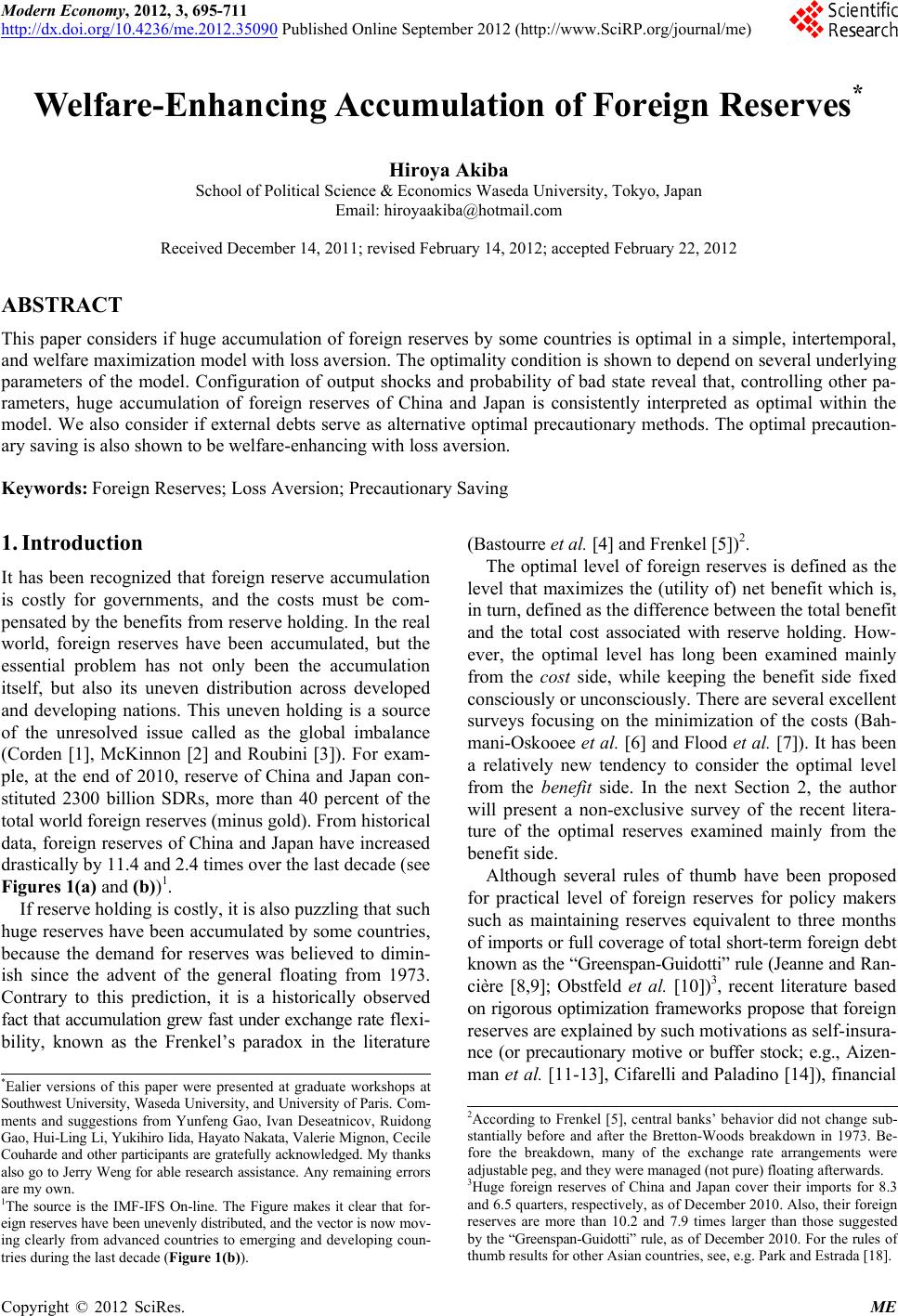Modern Economy, 2012, 3, 695-711
http://dx.doi.org/10.4236/me.2012.35090 Published Online September 2012 (http://www.SciRP.org/journal/me)
Welfare-Enhancing Accumulation of Foreign Reserves*
Hiroya Akiba
School of Political Science & Economics Waseda University, Tokyo, Japan
Received December 14, 2011; revised February 14, 2012; accepted February 22, 2012
ABSTRACT
This paper considers if huge accumulation of foreign reserves by some countries is optimal in a simple, intertemporal,
and welfare maximization model with loss aversion. The optimality condition is shown to depend on several underlying
parameters of the model. Configuration of output shocks and probability of bad state reveal that, controlling other pa-
rameters, huge accumulation of foreign reserves of China and Japan is consistently interpreted as optimal within the
model. We also consider if external debts serve as alternative optimal precautionary methods. The optimal precaution-
ary saving is also shown to be welfare-enhancing with loss aversion.
Keywords: Foreign Reserves; Loss Aversion; Precautionary Saving
1. Introduction
It has been recognized that foreign reserve accumulation
is costly for governments, and the costs must be com-
pensated by the benefits from reserve holding. In the real
world, foreign reserves have been accumulated, but the
essential problem has not only been the accumulation
itself, but also its uneven distribution across developed
and developing nations. This uneven holding is a source
of the unresolved issue called as the global imbalance
(Corden [1], McKinnon [2] and Roubini [3]). For exam-
ple, at the end of 2010, reserve of China and Japan con-
stituted 2300 billion SDRs, more than 40 percent of the
total world foreign reserves (minus gold). From historical
data, foreign reserves of China and Japan have increased
drastically by 11.4 and 2.4 times over the last decade (see
Figures 1(a) and (b))1.
If reserve holding is costly, it is also puzzling that such
huge reserves have been accumulated by some countries,
because the demand for reserves was believed to dimin-
ish since the advent of the general floating from 1973.
Contrary to this prediction, it is a historically observed
fact that accumulation grew fast under exchange rate flexi-
bility, known as the Frenkel’s paradox in the literature
(Bastourre et al. [4] and Frenkel [5])2.
The optimal level of foreign reserves is defined as the
level that maximizes the (utility of) net benefit which is,
in turn, defined as the difference between the total benefit
and the total cost associated with reserve holding. How-
ever, the optimal level has long been examined mainly
from the cost side, while keeping the benefit side fixed
consciously or unconsciously. There are several excellent
surveys focusing on the minimization of the costs (Bah-
mani-Oskooee et al. [6] and Flood et al. [7]). It has been
a relatively new tendency to consider the optimal level
from the benefit side. In the next Section 2, the author
will present a non-exclusive survey of the recent litera-
ture of the optimal reserves examined mainly from the
benefit side.
Although several rules of thumb have been proposed
for practical level of foreign reserves for policy makers
such as maintaining reserves equivalent to three months
of imports or full coverage of total short-term foreign debt
known as the “Greenspan-Guidotti” rule (Jeanne and Ran-
cière [8,9]; Obstfeld et al. [10])3, recent literature based
on rigorous optimization frameworks propose that foreign
reserves are explained by such motivations as self-insura-
nce (or precautionary motive or buffer stock; e.g., Aizen-
man et al. [11-13], Cifarelli and Paladino [14]), financial
*Ealier versions of this paper were presented at graduate workshops at
Southwest University, Waseda University, and University of Paris. Com-
ments and suggestions from Yunfeng Gao, Ivan Deseatnicov, Ruidong
Gao, Hui-Ling Li, Yukihiro Iida, Hayato Nakata, Valerie Mignon, Cecile
Couharde and other participants are gratefully acknowledged. My thanks
also go to Jerry Weng for able research assistance. Any remainingerrors
are my own.
1The source is the IMF-IFS On-line. The Figure makes it clear that for-
eign reserves have been unevenly distributed, and the vector is now mov-
ing clearly from advanced countries to emerging and developing coun-
tries during the last decade (Figure 1(b)).
2According to Frenkel [5], central banks’ behavior did not change sub-
stantially before and after the Bretton-Woods breakdown in 1973. Be-
fore the breakdown, many of the exchange rate arrangements were
adjustable peg, and they were managed (not pure) floating afterwards.
3Huge foreign reserves of China and Japan cover their imports for 8.3
and 6.5 quarters, respectively, as of December 2010. Also, their foreign
reserves are more than 10.2 and 7.9 times larger than those suggested
by the “Greenspan-Guidotti” rule, as of December 2010. For the rules o
f
thumb results for other Asian countries, see, e.g. Park and Estrada [18].
C
opyright © 2012 SciRes. ME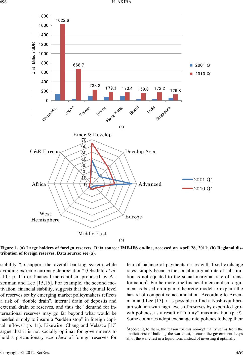

H. AKIBA
696
Foreign Reserve minus Gold (bil.SDR)
2001 Q1 2010 Q1
China,M.L.141.9 1622.6
Japan28.17 668.7
Taiwan87.8 233.8
Korea74.9 179.3
Hong Kon
g
90.9 170.4
Brazil27.1 159.8
India31.9 172.2
Singapore61.5 129.8
1622.6
668.7
233.8 179.3 170.4 159.8 172.2 129.8
0
200
400
600
800
1000
1200
1400
1600
China,M.L.
Japan
Taiwan
Korea
Hong Kong
Brazil
Indi a
Singapore
1800
2001 Q1
2010 Q1
Unit: Billion SD
R
(a)
0
10
20
30
40
50
60
70
Develop Asia
Advanced
Europe
Middle East
West
He misphere
Africa
C&E Europe
Emer & Develop
2001 Q1
2010 Q1
(b)
Figure 1. (a) Large holders of foreign reserves. Data source: IMF-IFS on-line, accessed on April 28, 2011; (b) Regional dis-
tribution of foreign reserves. Data source: see (a).
stability “to support the overall banking system while
avoiding extreme currency depreciation” (Obstfeld et al.
[10]: p. 11) or financial mercantilism proposed by Ai-
zenman and Lee [15,16]. For example, the second mo-
tivation, financial stability, suggests that the optimal level
of reserves set by emerging market policymakers reflects
a risk of “double drain”, internal drain of deposits and
external drain of reserves, and thus the “demand for in-
ternational reserves may go far beyond what would be
needed simply to insure a “sudden stop” in foreign capi-
tal inflows” (p. 11). Likewise, Chang and Velasco [17]
argue that it is not socially optimal for governments to
hold a precautionary war chest of foreign reserves for
fear of balance of payments crises with fixed exchange
rates, simply because the social marginal rate of substitu-
tion is not equated to the social marginal rate of trans-
formation4. Furthermore, the financial mercantilism argu-
ment is based on a game-theoretic model to explain the
hazard of competitive accumulation. According to Aizen-
man and Lee [15], it is possible to find a Nash-equilibri-
um solution with high levels of reserves by export-led gro-
wth policies, as a result of “utility” maximization (p. 9).
Some countries adopt exchange rate policies to keep their
4According to them, the reason for this non-optimality stems from the
implicit cost of building the war chest, because the government keeps
all of the war chest in a liquid form instead of investing it optimally.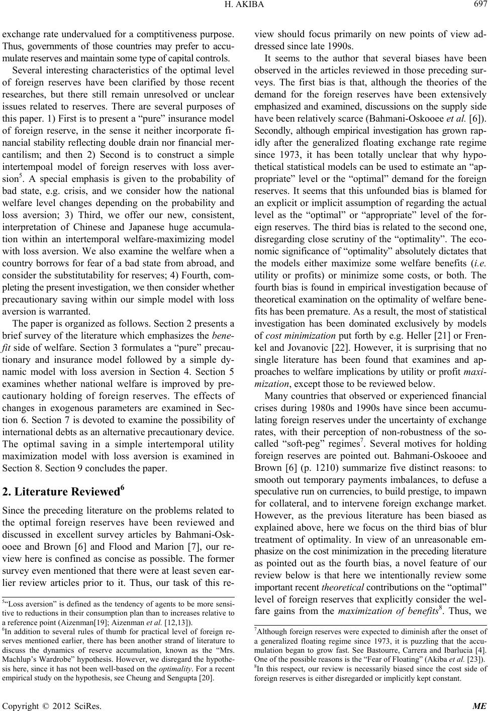

H. AKIBA 697
exchange rate undervalued for a comptitiveness purpose.
Thus, governments of those countries may prefer to accu-
mulate reserves and maintain some type of capital controls.
Several interesting characteristics of the optimal level
of foreign reserves have been clarified by those recent
researches, but there still remain unresolved or unclear
issues related to reserves. There are several purposes of
this paper. 1) First is to present a “pure” insurance model
of foreign reserve, in the sense it neither incorporate fi-
nancial stability reflecting double drain nor financial mer-
cantilism; and then 2) Second is to construct a simple
intertempoal model of foreign reserves with loss aver-
sion5. A special emphasis is given to the probability of
bad state, e.g. crisis, and we consider how the national
welfare level changes depending on the probability and
loss aversion; 3) Third, we offer our new, consistent,
interpretation of Chinese and Japanese huge accumula-
tion within an intertemporal welfare-maximizing model
with loss aversion. We also examine the welfare when a
country borrows for fear of a bad state from abroad, and
consider the substitutability for reserves; 4) Fourth, com-
pleting the present investigation, we then consider whether
precautionary saving within our simple model with loss
aversion is warranted.
The paper is organized as follows. Section 2 presents a
brief survey of the literature which emphasizes the bene-
fit side of welfare. Section 3 formulates a “pure” precau-
tionary and insurance model followed by a simple dy-
namic model with loss aversion in Section 4. Section 5
examines whether national welfare is improved by pre-
cautionary holding of foreign reserves. The effects of
changes in exogenous parameters are examined in Sec-
tion 6. Section 7 is devoted to examine the possibility of
international debts as an alternative precautionary device.
The optimal saving in a simple intertemporal utility
maximization model with loss aversion is examined in
Section 8. Section 9 concludes the paper.
2. Literature Reviewed6
Since the preceding literature on the problems related to
the optimal foreign reserves have been reviewed and
discussed in excellent survey articles by Bahmani-Osk-
ooee and Brown [6] and Flood and Marion [7], our re-
view here is confined as concise as possible. The former
survey even mentioned that there were at least seven ear-
lier review articles prior to it. Thus, our task of this re-
view should focus primarily on new points of view ad-
dressed since late 1990s.
It seems to the author that several biases have been
observed in the articles reviewed in those preceding sur-
veys. The first bias is that, although the theories of the
demand for the foreign reserves have been extensively
emphasized and examined, discussions on the supply side
have been relatively scarce (Bahmani-Oskooee et al. [6]).
Secondly, although empirical investigation has grown rap-
idly after the generalized floating exchange rate regime
since 1973, it has been totally unclear that why hypo-
thetical statistical models can be used to estimate an “ap-
propriate” level or the “optimal” demand for the foreign
reserves. It seems that this unfounded bias is blamed for
an explicit or implicit assumption of regarding the actual
level as the “optimal” or “appropriate” level of the for-
eign reserves. The third bias is related to the second one,
disregarding close scrutiny of the “optimality”. The eco-
nomic significance of “optimality” absolutely dictates that
the models either maximize some welfare benefits (i.e.
utility or profits) or minimize some costs, or both. The
fourth bias is found in empirical investigation because of
theoretical examination on the optimality of welfare bene-
fits has been premature. As a result, the most of statistical
investigation has been dominated exclusively by models
of cost minimization put forth by e.g. Heller [21] or Fren-
kel and Jovanovic [22]. However, it is surprising that no
single literature has been found that examines and ap-
proaches to welfare implications by utility or profit maxi-
mization, except those to be reviewed below.
Many countries that observed or experienced financial
crises during 1980s and 1990s have since been accumu-
lating foreign reserves under the uncertainty of exchange
rates, with their perception of non-robustness of the so-
called “soft-peg” regimes7. Several motives for holding
foreign reserves are pointed out. Bahmani-Oskooee and
Brown [6] (p. 1210) summarize five distinct reasons: to
smooth out temporary payments imbalances, to defuse a
speculative run on currencies, to build prestige, to impawn
for collateral, and to intervene foreign exchange market.
However, as the previous literature has been biased as
explained above, here we focus on the third bias of blur
treatment of optimality. In view of an unreasonable em-
phasize on the cost minimization in the preceding literature
as pointed out as the fourth bias, a novel feature of our
review below is that here we intentionally review some
important recent theoretical contributions on the “optimal”
level of foreign reserves that explicitly consider the wel-
fare gains from the maximization of benefits8. Thus, we
5“Loss aversion” is defined as the tendency of agents to be more sensi-
tive to reductions in their consumption plan than to increases relative to
a reference point (Aizenman[19]; Aizenman et al. [12,13]).
6In addition to several rules of thumb for practical level of foreign re-
serves mentioned earlier, there has been another strand of literature to
discuss the dynamics of reserve accumulation, known as the “Mrs.
Machlup’s Wardrobe” hypothesis. However, we disregard the hypothe-
sis here, since it has not been well-based on the optimality. For a recent
empirical study on the hypothesis, see Cheung and Sengupta [20].
7Although foreign reserves were expected to diminish after the onset o
f
a generalized floating regime since 1973, it is puzzling that the accu-
mulation began to grow fast. See Bastourre, Carrera and Ibarlucia [4].
One of the possible reasons is the “Fear of Floating” (Akiba et al. [23]).
8In this respect, our review is necessarily biased since the cost side o
f
foreign reserves is either disregarded or implicitly kept constant.

H. AKIBA
698
totally disregard empirical articles in our discussion below
simply because they have been exclusively examined
through the cost side of foreign reserves. One additional
new point of view is examination of effects of interna-
tional debts on the level of foreign reserves, as the mone-
tary authority (or government agencies) might determine
both of them jointly through the budget constraint.
Moreover, Aizenman [19,12] first formulates a model
for the optimal level of foreign reserves by applying a
microeconomic utility maximization problem. Using the
concept of “disappointment aversion” by Gull [24], he
derives the government’s optimal level of foreign re-
serves by applying an individual’s expected utility func-
tion that exhibits “disappointment” from a smaller con-
sumption than the certainty equivalent level under in-
come uncertainty. The “disappointment aversion” meas-
ure has been called “loss aversion” after expanding its
domain over total wealth. Applying the concept of “loss
aversion” within a framework of buffer stock and foreign
reserves, Aizenman [19,12] shows that the foreign re-
serves as buffer stock in fact depend on disappointment
aversion (or loss aversion) in a tractable way. Specifically,
it rigorously shows that the optimal foreign reserves are
increasing with loss aversion, and the optimal level is
likely to be positive under income uncertainty.
In order to show the importance of loss aversion, Ai-
zenman and Marion [11], recognizing that the Korean
financial crisis since 1997 was caused by a fall in will-
ingness of international loans due to a decrease in the
Korean reserve level, show that a change in reserves has
an asymmetric effect, especially when an expected large
fall in reserves causes a large reduction in the supply of
international credit when the private sector downgrades
its prior belief towards repayment possibilities or becomes
more pessimistic about the future level of reserve posi-
tion. This asymmetric effect is the essence of the notion
of disappointment (or loss) aversion.
Both Aizenman and Marion [12,13] and Alfaro and
Kanczuk [25] consider an intertemporal, 2-period, and
dynamic stochastic model under income uncertainty. They
examine whether a country, maximizing the present dis-
counted value of the expected utility, holds foreign re-
serves for a precautionary purpose. The novel feature of
the model lies in their assumption that the government
maximizes the country’s welfare by jointly choosing the
optimal levels of foreign reserves and international debts.
In the former article, the government finances its foreign
reserves’ costs by collecting taxes. Moreover, while the
former article shows that the optimal foreign reserve level
is unambiguously positive when the country’s historical
reserve position is zero, the latter article also calibrates
the optimal dynamic course of foreign reserves, showing
that the optimal level is zero. The differences reveal two
interesting facts toward the model. First the positive re-
serve level in the former article is shown only at the point
of time where the initial holding is zero, while the latter
article examines the future reserve level is zero. Second,
while the former article has not considered the possibility
of default, the latter article assumes it as a possible choice.
The common feature of both studies is that the optimal
reserves decrease as the discount factor decreases. This is
a plausible result, as it implies more consumption in an
earlier period and tilts the tax rates toward a later period.
Thus, international reserve holding must fall, while ex-
ternal borrowing must rise to satisfy the budget constraint.9
But, the latter article shows that both are not perfect sub-
stitutes because of possibility of default. Since the most
of the latter article’s results are based only on calibration
with specific assumptions of an isoelastic utility function
and GDP being fitted by an AR(1) process, and even
though their several robustness exercises, their conclu-
sion of the optimal level of foreign reserves being zero
remains to be explained in view of the large actual ac-
cumulation of foreign reserves in many developed, de-
veloping, and emerging economies.
Aizenman and Lee [15,16] consider whether foreign
reserves for a precautionary purpose is consistent with a
mercantilist interpretation. They distinguished two differ-
ent mercantilisms: financial and monetary. The former one
is characterized by direct subsidies, financial repressions,
or moral suasion, while the latter one hinges on hoarding
foreign reserves. As long as both mercantilisms have a
negative beggar-thy-neighbor externality associated with
costs, large reserve holding is inefficient. While their
article [15] deduces that monetary mercantilism is ob-
servationally near-equivalent to precautionary holding,
they come up from their regression in their article [16]
with a conclusion that the precautionary motive plays a
more visible role than the mercantilist motive represented
by the growth rate of real exports and national price lev-
els. Then, they construct a two-period dynamic model of
a private bank embodying a precautionary motive by
self-insurance. The model is similar in spirit to Aizenman
and Marion [12,13] that the bank borrows (accepts de-
posits) and either invests in real capital or hoards as re-
serves. Thus, the model is a straightforward application
of the familiar bank run model by Diamond and Dybvig
[26]. By maximizing the expected profits, they derive
that the optimal reserves are held up to the point where
the expected opportunity cost of hoarding reserves equals
the expected precautionary benefit. Then, they calculate
the optimal demand for deposit and the profit, and they
simulate it under a liquidity shock defined by fluctuations
in the ratio of reserves to deposit. They show a plausible
result that the reserve ratio increases with the volatility.
9According to Aizenman and Marion ([12]: p. 394), the effect of the
decrease in the discount factor is “very similar to the effect of political
uncertaint
y
or corru
p
tion.”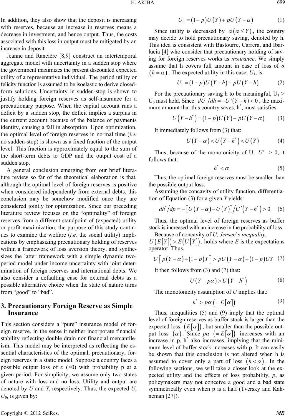

H. AKIBA 699




01UpUYpUY
In addition, they also show that the deposit is increasing
with reserves, because an increase in reserves means a
decrease in investment, and hence output. Thus, the costs
associated with this loss in output must be mitigated by an
increase in deposit.
Jeanne and Rancière [8,9] construct an intertemporal
aggregate model with uncertainty in a sudden stop where
the government maximizes the present discounted expected
utility of a representative individual. The period utility or
felicity function is assumed to be isoelastic to derive closed-
form solutions. Uncertainty in sudden-stop is shown to
justify holding foreign reserves as self-insurance for a
precautionary purpose. When the capital account runs a
deficit by a sudden stop, the deficit implies a surplus in
the current account because of the balance of payments
identity, causing a fall in absorption. Upon optimization,
the optimal level of foreign reserves in normal time (i.e.
no sudden-stop) is shown as a fixed fraction of the output
level. This fraction is approximately equal to the sum of
the short-term debts to GDP and the output cost of a
sudden stop.
A general conclusion emerging from our brief litera-
ture review so far of the theoretical elaboration is that,
although the optimal level of foreign reserves is positive
when considered independently from external debts, this
conclusion may be somehow modified once they are
considered jointly for optimization. Since our preceding
literature review focuses on the “optimality” of foreign
reserves from a different standpoint of (expected) utility
or profit maximization, the purpose of this study contin-
ues to examine the welfare (i.e. the social utility) impli-
cations by emphasizing precautionary holding of reserves
within a framework of loss aversion theory, and synthe-
sizes the latter framework with a simple dynamic two-
period model under income uncertainty with joint deter-
mination of foreign reserves and international debts. We
also consider a defaulting case for external debts as a
possible alternative choice when the state of nature turns
from “good” to “bad”.
3. Precautionary Foreign Reserve as Simple
Insurance
This section considers a “pure” insurance model of for-
eign reserve, in the sense it neither incorporate financial
stability reflecting double drain nor financial mercantile-
ism. This model may be interpreted as reflecting the es-
sential characteristics of the optimal, precautionary, for-
eign reserves in a static model. Suppose a country faces a
possible output loss of x (>0) with probability p at a
given period. For simplicity, we assume only two states
of nature with loss and no loss. Utility and output are
denoted by U and Y, respectively. Thus, the expected U,
U0, is given by:




Y  
(1)
Since utility is decreased by , the country
may decide to hold precautionary saving, denoted by h.
This idea is consistent with Bastourre, Carrera, and Ibar-
lucia [4] who consider that precautionary holding of sav-
ing for foreign reserves works as insurance. We simply
assume that h covers full amount in case of loss of α


h

. The expected utility in this case, U1, is:




11UpUYhpUY h

 (2)
For the precautionary saving h to be meaningful, U1 >
U0 must hold. Since

'0dU dhU Yh 
1, the maxi-
mum amount that this country saves, h*, must satisfies:



 
*1UY hpUYpUY

 (3)
It immediately follows from (3) that:




*
UYUY hUY   
U
(4)
Thus, because of the monotonicity of U,

> 0, it
follows that:
*
h

(5) 
Thus, the optimal foreign reserves must be smaller than
the possible output loss.
Assuming the concavity of utility function, differentia-
tion of Equation (3) for a given Y yields:



**
0dh dpUYUYU Yh 


 

(6)
Thus, the optimal level of foreign reserves as buffer
stock is increased with an increase in the probability of loss.
Because of concavity of U, Jensen’s inequality,








UEY EUY, holds where E is the expectations
operator. Thus,




11UpYpY pUYpUY    
 (7)
It then follows from (3) and (7) that:



*
UYpUY h   

(8)
The monotonicity assumption of U implies that:



*
hpE (9)

 
Thus, inequalities (5) and (9) imply that the optimal
level of foreign reserves as buffer stock is larger than the
expected loss




E

, but smaller than the possible out-
put loss




E



. Since pα



h
increases with an
increase in p, h* also increases, implying that the mini-
mum level of buffer stock increases with p. It can easily
be shown that this conclusion is not altered when h is
assumed to cover only a part of loss


neman [27]).
. In the
following sections, we will take a closer look at the ex-
pected utility and the effects of loss probability, p, as
policymakers may not conceive a good and a bad state
symmetrically even when p is a half (Tversky and Kah-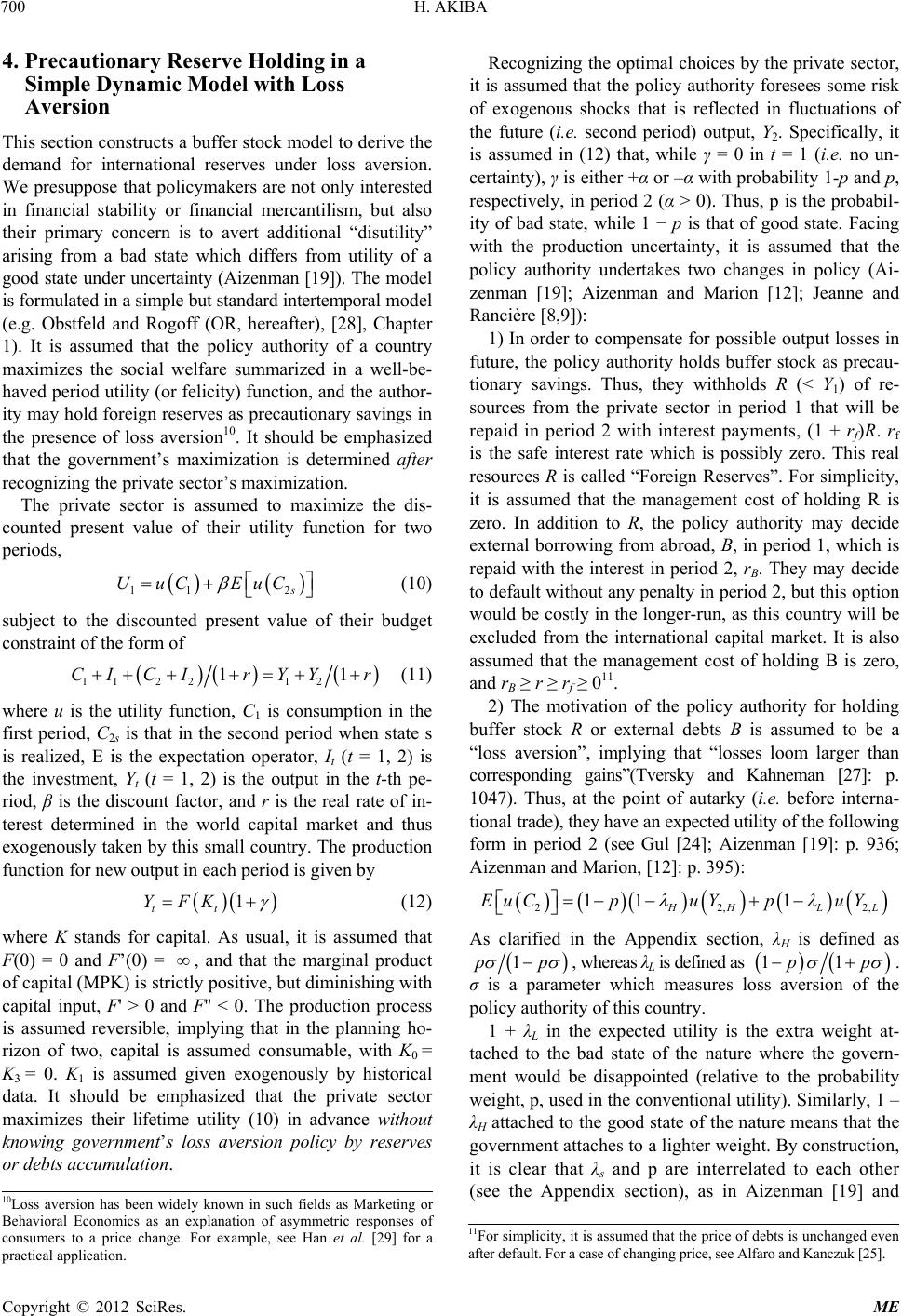

H. AKIBA
700
4. Precautionary Reserve Holding in a
Thucts a buffer stock model to derive the
dis-
co
 
11 2s
UuC EuC 



(10)
subject to the discounted present value of

Simple Dynamic Model with Loss
Aversion
is section constr
demand for international reserves under loss aversion.
We presuppose that policymakers are not only interested
in financial stability or financial mercantilism, but also
their primary concern is to avert additional “disutility”
arising from a bad state which differs from utility of a
good state under uncertainty (Aizenman [19]). The model
is formulated in a simple but standard intertemporal model
(e.g. Obstfeld and Rogoff (OR, hereafter), [28], Chapter
1). It is assumed that the policy authority of a country
maximizes the social welfare summarized in a well-be-
haved period utility (or felicity) function, and the author-
ity may hold foreign reserves as precautionary savings in
the presence of loss aversion10. It should be emphasized
that the government’s maximization is determined after
recognizing the private sector’s maximization.
The private sector is assumed to maximize the
unted present value of their utility function for two
periods,
their budget
constraint of the form of

11221 2
11r YYr  (11)
where u is the utility function, C1 is consumption in
CICI 
the
first period, C2s is that in the second period when state s
is realized, E is the expectation operator, It (t = 1, 2) is
the investment, Yt (t = 1, 2) is the output in the t-th pe-
riod, β is the discount factor, and r is the real rate of in-
terest determined in the world capital market and thus
exogenously taken by this small country. The production
function for new output in each period is given by



1
tt
YFK

 (12)
where K stands for capital. As usual, it is assum
al choices by the private sector,
it is assumed that the policy authority foresees some risk
of exogenous shocks that is reflected in fluctuations of
the future (i.e. second period) output, Y2. Specifically, it
is assumed in (12) that, while γ = 0 in t = 1 (i.e. no un-
certainty), γ is either +α or –α with probability 1-p and p,
respectively, in period 2 (α > 0). Thus, p is the probabil-
ity of bad state, while 1 − p is that of good state. Facing
with the production uncertainty, it is assumed that the
policy authority undertakes two changes in policy (Ai-
zenman [19]; Aizenman and Marion [12]; Jeanne and
Rancière [8,9]):
1) In order to compensate for possible output losses in
future, the policy authority holds buffer stock as precau-
tionary savings. Thus, they withholds R (< Y1) of re-
sources from the private sector in period 1 that will be
repaid in period 2 with interest payments, (1 + rf)R. rf
is the safe interest rate which is possibly zero. This real
resources R is called “Foreign Reserves”. For simplicity,
it is assumed that the management cost of holding R is
zero. In addition to R, the policy authority may decide
external borrowing from abroad, B, in period 1, which is
repaid with the interest in period 2, rB. They may decide
to default without any penalty in period 2, but this option
would be costly in the longer-run, as this country will be
excluded from the international capital market. It is also
assumed that the management cost of holding B is zero,
and rB ≥ r ≥ rf ≥ 011.
2) The motivation of the policy authority for holding
buffer stock R or external debts B is assumed to be a
“loss aversion”, implying that “losses loom larger than
corresponding gains”(Tversky and Kahneman [27]: p.
1047). Thus, at the point of autarky (i.e. before interna-
tional trade), they have an expected utility of the following
form in period 2 (see Gul [24]; Aizenman [19]: p. 936;
Aizenman and Marion, [12]: p. 395):
ed that
F(0) = 0 and F’(0) = , and that the marginal product
of capital (MPK) is strictly positive, but diminishing with
capital input, F' > 0 and F'' < 0. The production process
is assumed reversible, implying that in the planning ho-
rizon of two, capital is assumed consumable, with K0 =
K3 = 0. K1 is assumed given exogenously by historical
data. It should be emphasized that the private sector
maximizes their lifetime utility (10) in advance without
knowing government’s loss aversion policy by reserves
or debts accumulation.
Recognizing the optim










22,2,
11 1
H
HLL
EuCpuY puY   

As clarified in the Appendix section, λH is defined as


1pp  , whereas λL is defined as




11pp

 .
σ is a parameter which measures loss aversion of the
policy authority of this country.
1 + λL in the expected utility is the extra weight at-
tached to the bad state of the nature where the govern-
ment would be disappointed (relative to the probability
weight, p, used in the conventional utility). Similarly, 1 –
λH attached to the good state of the nature means that the
government attaches to a lighter weight. By construction,
it is clear that λs and p are interrelated to each other
(see the Appendix section), as in Aizenman [19] and
10Loss aversion has been widely known in such fields as Marketing or
Behavioral Economics as an explanation of asymmetric responses o
f
consumers to a price change. For example, see Han et al. [29] for a
p
ractical application.
11For simplicity, it is assumed that the price of debts is unchanged even
after default. For a case of changing price, see Alfaro and Kanczuk [25].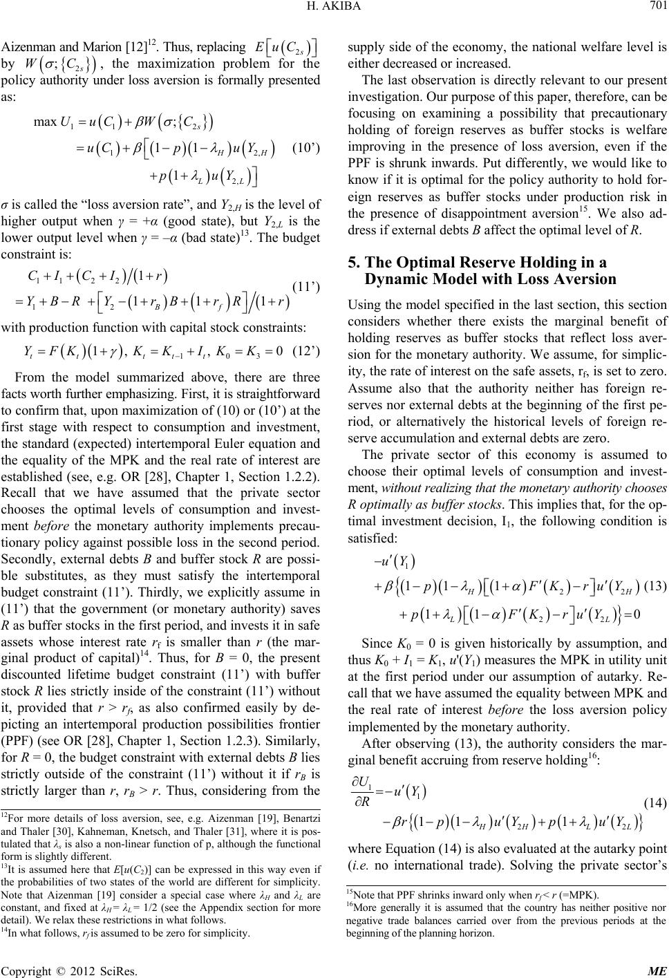

H. AKIBA 701
Aizenman and Marion [12]12. Thus, replacing


2s
EuC




by



2
;s WC  , the maximization problem for the
policy authority under loss aversion is formally presented
as:




 
 
11 2
12,
2,
max ;
11
1
s
HH
LL
UuCWC
uCp uY
puY








 
(10’)
σ is called the “loss aversion rate”, and Y2,H is the level of
higher output when γ = +α (good state), but Y2,L is the
lower output level when γ = –α (bad
co
state)13. The budget
nstraint is:




  
112 2
12
1
111
Bf
CICIr
YBRYrBrRr
 

 

(11’)
with production function with capital stock constraints:
 
levels of consumption and invest-
m
r than r (the mar-
ginal product of capital). Thus, for B = 0, the presen
discounted lifetime budget constraint (11’) with buffe
med easilye
fare level is
er decreased o
stigation. Our purpose of this paper, therefore, can be
focusing on examining a possibility that precautionary
holding of foreign reserves as buffer stocks is welfare
improving in the presence of loss aversion, even if the
PPF is shrunk inwards. Put differently, we would like to
know if it is optimal for the policy authority to hold for-
eign reserves as buffer stocks under production risk in
the presence of disappointment aversion15. We also ad-
dress if external debts B affect the optimal level of R.
5. The Optimal Reserve Holding in a
Dynamic Model with Loss Aversion
Using the model specified in the last section, this section
considers whether there exists the marginal benefit of
holding reserves as buffer stocks that reflect loss aver-
sion for the monetary authority. We assume, for simplic-
ity, the rate of interest on the safe assets, rf, is set to zero.
Assume also that the authority neither has foreign re-
serves nor external debts at the beginning of the first pe-
riod, or alternatively the historical levels of foreign re-
serve accumulation and external debts are zero.
The private sector of this economy is assumed to
choose their optimal levels of consumption and invest-
ment, without realizing that the monetary authority chooses
R optimally as buffer stocks. This implies that, for the op-
timal investment decision, I1, the following condition is
satisfied:
103
1, , 0
tt ttt
YFKKKIKK 


(12’)
From the model summarized above, there are three
facts worth further emphasizing. First, it is straightforward
to confirm that, upon maximization of (10) or (10’) at the
first stage with respect to consumption and investment,
the standard (expected) intertemporal Euler equation and
the equality of the MPK and the real rate of interest are
established (see, e.g. OR [28], Chapter 1, Section 1.2.2).
Recall that we have assumed that the private sector
chooses the optimal
ent before the monetary authority implements precau-
tionary policy against possible loss in the second period.
Secondly, external debts B and buffer stock R are possi-
ble substitutes, as they must satisfy the intertemporal
budget constraint (11’). Thirdly, we explicitly assume in
(11’) that the government (or monetary authority) saves
R as buffer stocks in the first period, and invests it in safe
assets whose interest rate rf is smalle
14 t
r
stock R lies strictly inside of the constraint (11’) without
it, provided that r > rf, as also confir by d-
picting an intertemporal production possibilities frontier
(PPF) (see OR [28], Chapter 1, Section 1.2.3). Similarly,
for R = 0, the budget constraint with external debts B lies
strictly outside of the constraint (11’) without it if rB is
strictly larger than r, rB > r. Thus, considering from the
supply side of the economy, the national wel
eithr increased.
The last observation is directly relevant to our present
inve


 

 

1
22
22
11 1
110
HH
LL
uY
pFKruY
pFKruY





  



 

(13)
Since K0 = 0 is given historically by assumption, and
thus K0 + I1 = K1, u'(Y1) measures the MPK in utility unit
at the first period under our assumption of autarky. Re-
call that we have assumed the equality between MPK and
the real rate of interest before the loss aversion policy
implemented by the monetary authority.
After observing (13), the authority considers the mar-
ginal benefit accruing from reserve holding16:

  
1
1
22
11 1
HH LL
UuY
R
rpuYp uY
 






(14)
where Equation (14) is also evaluated at the autarky point
(i.e. no international trade). Solving the private sector’s
12For more details of loss aversion, see, e.g. Aizenman [19], Benartzi
and Thaler [30], Kahneman, Knetsch, and Thaler [31], where it is pos-
tulated that λs is also a non-linear function of p, although the functional
form is slightly different.
13It is assumed here that E[u(C2)] can be expressed in this way even i
f
the probabilities of two states of the world are different for simplicity.
N
ote that Aizenman [19] consider a special case where λH and λLare
constant, and fixed at λH = λL = 1/2 (see the Appendix section for more
detail). We relax these restrictions in what follows.
14In what follows, r
f
is assumed to be zero for simplicity.
15Note that PPF shrinks inward only when rf < r (=MPK).
16More generally it is assumed that the country has neither positive nor
negative trade balances carried over from the previous periods at the
beginning of the planning horizon.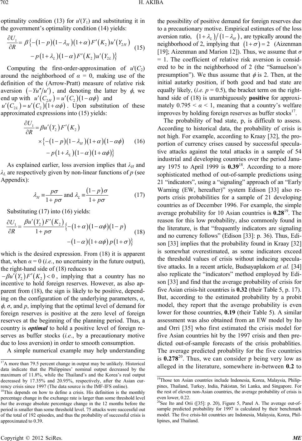

H. AKIBA
702
optimality condition (13) for u'(Y1) and substituting it in
the government’s optimality condition (14) yields:
  


1
22
11 1
HH
UpFKuY
R


 
 (15)
the (Arrow-Pratt) measure of relative risk
on


22
11
LL
pF KuY 

 
Computing the first-order-approximation of u'(C2)
around the neighborhood of α = 0, making use of the
definition of
aversi

Yu u
 
, and denoting the latter by  , we
with

end up


22
1
H
uC uC



 and

22
1C

u
L
uC



. Upon substitution of these

approximated expressions into (15) yields:
 
   
  
11 11
111
H
L
p
p
1
22
UuYF K
R




   

(16)
As explained earlier, loss aversion implies that λH and
λL are respectively given by non-linear functions of p (see
Appendix):




1
and
11
HL
p
p
pp








(17)
Substituting (17) into (16) yields:
 

 
22
111 1
1
111
uYF K
Up
Rp
p









 
(18)
which is the desired expression. From (18) it is apparent
that, when α = 0 (i.e., no uncertainty in the future output),
the right-hand side of (18) reduces to
 
22
0uY F K 

 , implying that a country has no
incentive to hold foreign reserves. However, as also ap-
parent from (18), the sign is likely to be positive, depend-
ing on the configuration of the underlying parameters, α,
 , σ, and p, implying that the optimal level of demand for
foreign reserves is positive at the zero level of foreign
reserves at the beginning of the planning period. Thus, a
country is optimal to hold a positive level of foreign re-
serves as buffer stocks (i.e., by a precautionary motive
due to loss aversion) in order to smooth consumption.
A simple numerical example may help understanding
the possibility of positive demand for foreign reserves due
to a precautionary motive. Empirical estimates of the loss
aversion ratio,




11
LH

 , are typically around the
neighborhood of 2, implying that

12   (Aizenman
[19]; Aizenman and Marion 12]). Thus, we assume that σ
= 1. The coefficient of relative risk aversion is consid-
ered to be in the neighborhood of 2 (the “Samuelson’s
presumption”). We thus assume that
 is 2. Then, at the
e right-
ha pproxi-
a more
so
obability for 10 Asian countries is 0.28 . The
reason for this low probability, also commonly found in
the literature, is that “frequently indicators are signaling
and no currency follows” (Edison [33]: p. 36). Thus,
son [33] implies that the probability found in Kraay [32]
is somewhat overestimated, as some indicators exceed
th
m
. A similar
assessment was also obtained from an EW model by Ito
and Orri [35] who first estimated the crisis mode
five Asian countries hit by the 1997 crisis and then
dicted out-of-sample forecasts of the crisis probablities.
initial autarky position, if both good and bad state are
equally likely, (i.e. p = 0.5), the bracket term on th
nd side of (18) is unambiguously positive for a
mately 0.795 < α < 1, meaning that a country’s welfare
improves by holding foreign reserves as buffer stocks17.
The probability of bad state, p, is difficult to assess.
According to historical data, the probability of crisis is
not high. For example, according to Kraay [32], the pro-
portion of currency crises caused by successful specula-
tive attacks against the total attacks in a sample of 54
industrial and developing countries over the period Janu-
ary 1975 to April 1999 is 0.3918. According to
phisticated method of out-of-sample predictions using
21 “indicators”, using a “signaling” approach of an “Early
Warning (EW, hereafter)” system Edison [33] also re-
ports crisis probabilities for a sample of 21 developing
countries as of December 1996. For example, the simple
average pr19
Edi -
e threshold values of crisis without inducing specula-
tive attacks. In a recent article, Budsayaplakorn et al. [34]
also replicate the “indicators” method employed by Edi-
son [33] and find that the average probability of crisis for
five Asian crisis-hit countries is 0.32 (their Table 5, p. 17).
But, according to the estimated probability by a probit
odel, they report that the average probability is even
lower for those countries, 0.19 (their Table 5)
l for
pre-
The average predicted probablity for the five countries
is 0.27820. Thus, we can consider p being very low as
alleged in the literature, somewhere in-between 0.2 to
19Those ten Asian countries include Indonesia, Korea, Malaysia, Philip-
p
ines, Thailand, Turkey, India, Pakistan, Sri Lanka, and Singapore. Fo
r
the rest of eleven non-Asian countries, the average probability of crisis is
even lower, 0.22.
verage out-of-
17A more than 79.5 percent change in output may be unlikely. Historical
data indicate that the Philippines’ nominal output decreased by the
maximum of 11.8%, while the Thailand’s and the Korea’s real output
decreased by 17.35% and 20.95%, respectively, after the Asian cur-
rency crisis since 1997 (The data source is the IMF-IFS online).
18This depends on how to define a crisis. His definition is the monthly
p
ercentage change in the exchange rate is larger than some threshold level
but the average absolute percentage change in the 12 months before the
p
eriod is smaller than some threshold level. 75 attacks were successful out
of the total of 192 episodes, and thus the probability o
20See Ito and Orii ([35]: p. 20), Figure 5, Panel A. The a
sample predicted probability for 1997 is calculated by their benchmark
model. The five crisis-hit countries are Indonesia, Malaysia, Korea, Phil-
lipines, and Thailand.
f successful crisis is
approximated to 0.39.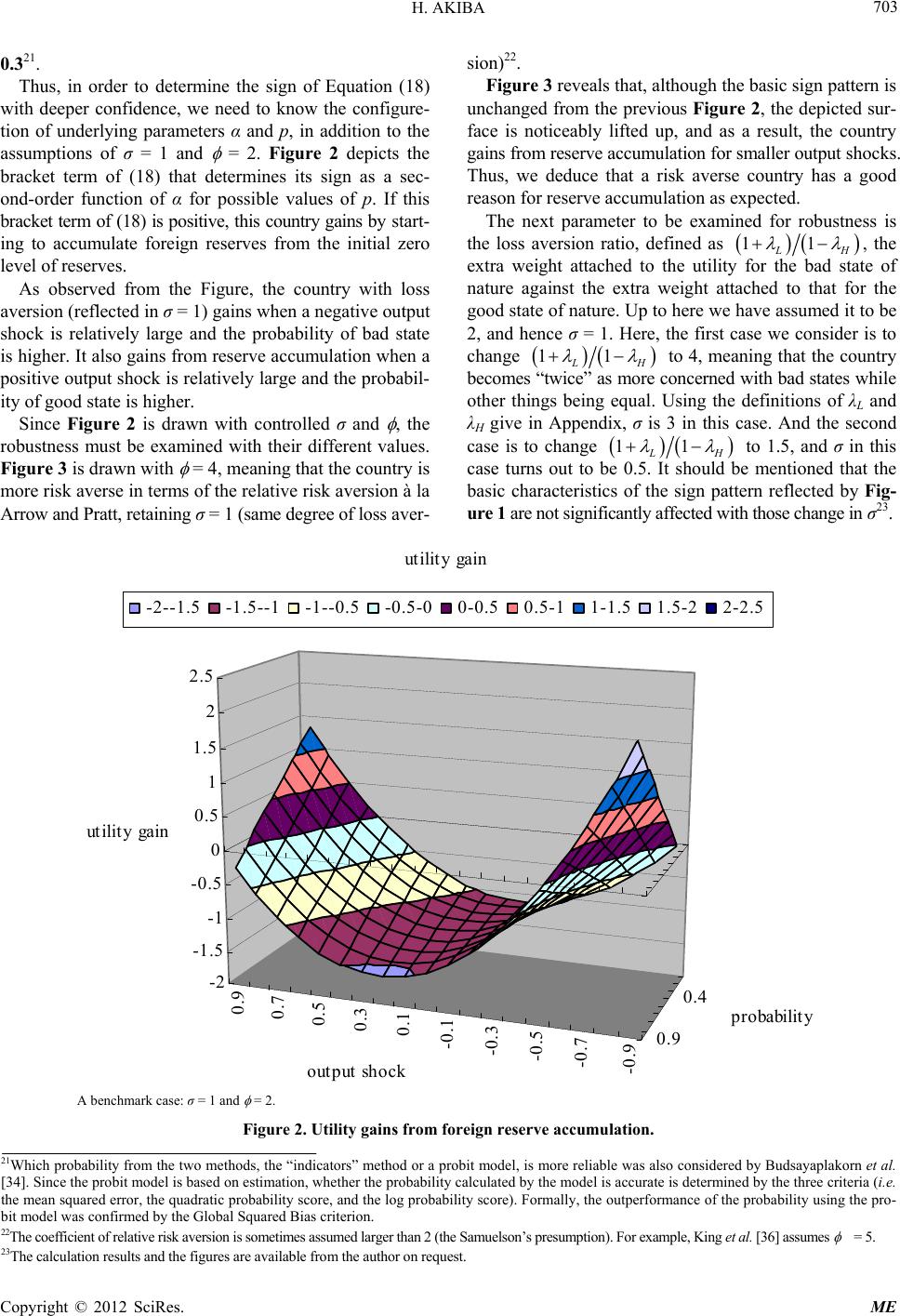

H. AKIBA
ME
703
0.321.
Thus, in order to determine the sign of Equatio
with deeper confidence, we need to know the confi
tion of underlying parameters α and p, in addition to the
as
m of (18)
ulate foreign reserves froinitial zero
level of reserves.
try with loss
aversion (reflected in σ = 1) gains when a negative output
shock is relatively large and the probability of bad state
is higher. It also gains from reserve accumulation w
positive output shock is relatively large and the p
ity of good state is higher.
Since Figure 2 is drawn with controlled σ and  , the
ro
erse in terms of the relative risk aversion à la
Arrow and Pratt, retaining σ = 1 (same degree of loss aver-
e basic s
sion)22.
Figure 3 reveals that, although thign pattern is
unchanged from the previous Figure 2, the depicted sur-
face is noticeably lifted up, and as a result, the country
gains from reserve accumulation for smaller output shocks.
Thus, we deduce that a risk averse country has a good
reason for reserve accumulation as expected.
The next parameter to be examined for robustness is
the loss aversion ratio, defined as
 
11
L
H

 , the
extra weight attached to the utility for the bad state of
nature against the extra weight attached to that for the
n (18)
gure-
sumptions of σ = 1 and  = 2. Figure 2 depicts the
bracket term of (18) that determines its sign as a sec-
ond-order function of α for possible values of p. If this
bracket teris positive, this country gains by start-
ing to accumm the
As observed from the Figure, the coun
good state of nature. Up to here we have assumed it to be
2, and hence σ = 1. Here, the first case we consider is to
change




11
L
H

  to 4, meaning that the country
becomes “twice” as more concerned with bad states while
other things being equal. Using the definitions of λL and
λH give in Appendix, σ is 3 in this case. And the second
case is to change




11
L
H

  to 1.5, and σ in this
case turns out to be 0.5. It should be mentioned that the
basic characteristics of the sign pattern reflected by Fi g-
ure 1 are not significantly affected with those change in σ23.
hen a
robabil-
bustness must be examined with their different values.
Figure 3 is drawn with  = 4, meaning that the country is
more risk av
0.
0.
0.5
0.3
0.1
-0.1
9
7
-0.3
-0.5
-0.7
.9-0
0.9
0.4
-2
-1.5
-1
-0.5
0
0.5
1
1.5
2
utility gain
2.5
pr obability
ainutility g
-2--1.5 -1.5--1 -1--0.5 -0.5-0 0-0.5 0.5-1 1-1.5 1.5-22-2.5
output shock
A benchmark case: σ = 1 and  = 2.
Figure 2. Utility gains from foreign reserve accumulation.
21Which probability from the two methods, the “indicators” method or a p
[34]. Since the probit model is based on estimation, whether the probabili
the mean squared error, the quadratic probability score, and the log proba
bit model was confirmed by the Global Squared Bias criterion.
22The coefficient of relative risk aversion is sometimes assumed larger than 2 (
23The calculation result
rob
ty c
bili
the S
s and the fi
it model, is more reliable was also considered by Budsayaplakorn et al.
alculated by the model is accurate is determined by the three criteria (i.e.
ty score). Formally, the outperformance of the probability using the pro-
amuelson’s presumption). For example, King et al. [36] assumes  = 5.
g
ures are available from the author on re
q
uest.

H. AKIBA
704
Thus, it is apparent from Figures 1 and 2 that the coun-
try gains from reserve accumulation a) for higher prob-
ability of bad state with higher negative output fluctua-
tion, and also b) for higher probability of good state with
higher positive output fluctuation. But the country looses
by reserve accumulation when output shock is small,
regardless of the probability of bad state. To confirm this
relative irresponsiveness of change in utility with respect
to
ing a larger weight to the bad
st
be
cumulation
of
low, since Chin
e that almost o
loss aversion, we perform additional robustness exer-
cise with a larger σ = 7, other things being equal. The
result with this strong emphasis on loss aversion parameter,
however, does not significantly affect the sign pattern
depicted by Figure 2 or 3. This suggests that the country
may not gain by simply add
ate in their utility function24.
This finding may offer a new interpretation for huge
foreign reserve accumulation by both China and Japan,
although they have been very much different not only in
political systems, but also economic aspects: China has
en a developing country with a high output growth rate,
but their per capita income has still remained very low.
On the other hand, Japan has been a member of the OECD
with a higher per capita income, but it has been suffering
from a stagnant economy (deflation) for more than twenty
years25. For these two countries with high ac
foreign reserves, our analysis offers a consistent ex-
planation for the “optimality”.
For a remarkable increase in Chinese foreign reserve
accumulation, it can be argued that, because of prolonged
steady rate of economic growth, α (a change in output), is
relatively large, while the probability of bad state (or cri-
sis), p, isa has been free from speculative
attacks because of relatively strict capital controls26. Thus,
it has been “optimal” for China to accumulate huge for-
eign reserves from the standpoint of loss aversion. It is
surprising to realizpposite reasons may
apply for large Japanese foreign reserve accumulation:
Because of the “lost two decades” of economic slump, –α
0.9
0.7
0.5
0.3
0.1
-0.1
-0.3
-0.5
-0.7
-0.9
0.9
0.4
-4
-2
0
2
4
6
8
10
utility gain
output shock
probability
utilitainy g
-4--2 -2-0 0-2 2-44-66-88-10
for
σ = 1 and  = 4. Figure 3. Utility gains from eign reserve accumulation.
24The most notable change from Figure 2 or 3 is that the slope of the surface is steeper in this case. The calculation result and the Figure are also available
on request.
25The Chinese and the Japanese per capita incomes in 2010 were US$4382.14 and US$42820.39, respectively, according to the IMF’s World Economic
Outlook (April, 2011).
26The Chinese average growth rate of the last decade (2002-2011) is 10.6 % (IMF-World Economic Outlook, April, 2011). Thus, China is an example o
f
case (a).

H. AKIBA 705
(<0) is relatively large in absolute value, while p has been
alleged to be large because of huge unsettled national
debts, almost 600 trillion yen (more than 120 percent of
nominal GDP) at the end of 200927. Thus, it may be rea-
sonable to understand why Japan has such a large “opti-
mal” accumulation of foreign reserves for a reason of loss
aversion, even though this interpretation may be reason-
able in hindsight once we recall that Japan has been blamed
for attaining the unprecedented high rate of economic
growth by increasing its exports like “concentrated heavy
rain”, or by “mercantilism”.
The next question to ask is how much foreign reserves
to accumulate as the “optimal” level. The answer has
al
6. Effects of Exogenous Changes on the
Optimal Reserves
This section examines the effects of exogenous shifts in
the four underlying parameters, and explores if a policy
of holding of foreign reserves at autarky is much more
legitimate and convincing. The results are summarized in
Panel A of Table 1.
6.1. An Increase in p
The first exercise is the effect of an exogenous increase
in the probability of bad state, p. Partial differentiation of
(18) with respect to p yields:
ready been given in our discussion in Section 3, where
we have found that the optimal precautionary savings as
buffer stock should be larger than the expected loss (see
Equation (9)) but smaller than the possible output loss
(see Equation (5))28.
 
 

1
22
1
221
1
uY F K
U
pR p










 
 (19)
which is negative for  = 2 and σ = 1. In other words,
when the probability of a bad state is more likely to in-
crease, the desirability of holding foreign reserves for a
precautionary purpose is diminished. This is plausible,
ation would be possible
w
to the probability of state of the nature.
6.2. An Increase in σ
The second exercise is an effect of increase in a parame-
ter which measures loss aversion of the policy authority
of this country, i.e. σ. Partial differentiation of (18) with
respect to σ yields:
because if the country holds foreign reserves, the total
spending would be reduced in a worse situation under the
risk of a higher probability of a bad state. This character-
istic is visualized clearly in Figure 2, where the utility
surface has a slope downward with the probability of bad
state, p.
However, another interpret
hen the (Arrow-Pratt) measure of relative risk aversion
 is smaller than unity. This in fact is equivalent to a
qualification made by Aizenman [19] (p. 943) that “the
concavity of the marginal utility is playing only a secon-
dary role”. Needless to say, (19) is also positive for  = 0,
meaning that the desirability of holding foreign reserves
is increased when the instantaneous (period) utility func-
tion is a linear function of consumption. If (19) is evalu-
ated at the initial point where α = 0 (i.e. no output uncer-
tainty), the whole expression reduces to 0, implying that
the desirability of holding foreign reserves is insensitive




 

22
1
221 1
1
uY F K
Upp
Rp










 (20)
which is negative for  = 2. Thus, the desirability of
holding foreign reserves diminishes for a higher measure
of loss aversion. This is also plausible, as the partial de-
rivatives of λH and λL in (17) with respect to σ are shown
to be positive for the former, but zero for the latter for p
= 0.5. Thus, for a higher measure of loss aversion σ, the
country attaches a higher weight for a good state, but an
unchanged weight for a bad state, implying that the coun-
try’s precautionary motive for holding foreign reserves is
weaker than otherwise.
However, (20) is positive when  < 1. This implies
that, if the preceding remark on the case (1) by Aizenman
[19] is plausible, the desirability of holding foreign re-
serves increases for a higher measure of loss aversion. A
similar interpretation to the preceding case (1) applies to
this case when the instantaneous (period) utility function
f consumption. Since a mar-
wise. Also, if (20) is evaluated at the initial point where α
sitive to loss aversion.
27The Japanese average annual growth rate of the “lost two decades”
(1992-2011) is only 0.87%. The lowest growth rate is –6.29% in 2009
(IMF-World Economic Outlook, April, 2011). According to Figure 2,
utility is increased by reserve accumulation at a point where p= 0.6 and
α = –0.6. This “indifference curve” shows the same utility for a lower p
with a higher α. A similar indifference relation is observed in Figure 3
where, for example, p = 0.8 with α = –0.3. Thus, Japan is an example o
f
case (bthe Bloomsberg’s report dated April 21, 2011
(http://www.bloomm/news), the
28
J
arch 11, 2011 is estimated as 16.9 trillion yen, about 3.5% o
is closer to a linear function o
ginal increase in loss aversion for a linear utility function
implies a decrease in the expected utility level, the desir-
). Accroding to
sberg.co “sovereign vulnerability index
ranks Japan as the second most vulnerable”, next to Greece. The USA
was ranked 5th.
According to the press release by the Japanese Cnet Office dated
une 24, 2011, the total loss incurred by the “Great East Japan Earth-
quake” on M
abi ability of holding foreign reserves increases than other-
= 0, the whole expression reduces to 0, i.e. the desirabil-
ity of holding foreign reserves as a buffer stock is insen-
f
t the end of 2010, while that of Chine was 49%.
11)).
the 2010 nominal GDP (479.2 trillion yen). The Japanese foreign reserve
ratio to GDP was 19% a
(Author’s calculation based on the IMF’s World Economic Outlook
(April, 20

H. AKIBA
706
ts o
nel
Fores)
Table 1. Comparative statics results for benefi
Pa
Parameter R (
f foreign reserves (R) and external debts (B).
A
eign Reserv
p



12
222
1
Uu
FK
pR p



 


 


1 
 

1  
 
σ


12
222
1FK
Rp 



1 1p   
Uu p 







 

α



12
2
1
Uu
FK p
Rp


1
 

1121p p

   



  
 
 
 

φ



12
Uu
FK


 


221
1Rp 


1 1p p    





 

δ -
β
 

2
1
21
1
uY
UFK
Bp



  


 

 

1 [11 21p   
Note: Evaluated at R = B = 0.
Panel B
nal Debts): No Defaulting B (International Debts): Defaulting* Parameter B (Internatio
p

 
12
221 1
1
Uu
FK
pB p



  


 
 

2
 
21
2
pB 2
91 211
1
uFK
p
 U

 



 








σ

 
21 1p
 



12
22
Uu
FK p
B



  



 

2
1p 


1
2
B 

2
121 1
1
u
pp FK
p
 



U 








α


  

2
2
1
11121
FK
p
pp p

1
U
B
u







 

 







U
B
F

 



211
1211K pppp

1p
1
2
u



  














φ




12
2
1
211 (1)
Uu
FK
Rp
pp




  


 





 

2
2211 11
1
u
FKpp p
p

1
R
U




  

 




δ -




  
2
2
1112
1
u
pFK
p
 




1
B

U



 

 




β



2
2
1
1111 21
B
uFK
p
p







   

1
U 

 

1
2
(121 11
U
B
2
1
u
p

) 1 11
F
Kp p










  




 








Note: Evaluated * at R = B = 0. means evaluated at rB = 0 and δ = 0.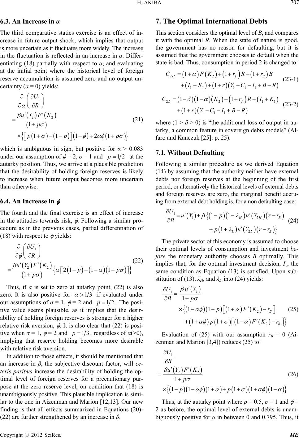

H. AKIBA 707
6.3. An Increase in α
The third com
crease in future output shock, which implies that outp
is more uncertain as it fluctuates more widely. The increase
in the fluctuation is reflan increase in α. Diffe
entiating (18) partially with respect to α, and evaluating
at the initial point where the historical level of foreign
reserve accumulation is assumed zero and no output un-
certainty (α = 0) yields:
parative statics exercise is an effect of in-
ut
ected in r-
 


1
22
1
111
U
R
uY F K
p
pp



 

21p


 
(21)
which is ambiguous in sign, but positive for α > 0.083
under our assumption of 
 







= 2, σ = 1 and 12p at the
autarky position. Thus, we arriplausible prediction
that the desirability of holding foreign reserves is likely
to increase when future outes more uncertain
than otherwise.
6.4. An Increase in
The fourth and the final exercise is an effect of increase
itudes milar pro-
cedure as in the previous cases, partial differentiation of
(18) with respect to
 yields:
ve at a
put becom

in the att towards risk,  . Following a si
 
 

1
22
211 1
1
U
R
uYF Kpp
p



 



 


(22)
Thus, if α is set to zero at autarky point, (22) is also
zero.

 
It is also positive for 13

 if evaluated under
our assumptions nd of σ = 1,  = 2 a12p. The posi-
tive value see it implies that the desir-
ability of holdirves is stronger for a higher
relative riskalso clear that (22) is posi-
tive when σ =
ms plausible,
ng foreign rese
aversion, 
1,  = 2
as
. It is
and 13p

, regardless of α(>0),
iming that reser becomes more desirable
with relative risk aversion.
In addition to those effects, it should be mentioned that
an increase in β, the subjective discount factor, will ce-
teris paribus increase the desirability of holding the op-
timal level of foreign reserves for a precautionary pur-
pose at the zero reserve level, on condition that (18) is
unambiguously positive. This plausible implication is simi-
lar to the one in Aizenman and Marion [12,13]. Our new
finding is that all effects summarized in Equations (20)-
(22) are further strengthened by an increase in β.
7. The Optimal International Debts
nd compares
ith the optimal R. When the state of nature is good,
the government has no reason for defaulting, but it is
t the government chooses to default when the
state is bad. Thus, consumption in period 2 is changed to:

plyve holding
This section considers the optimal level of B, a
it w
assumed tha



 
22
11 111
111
1
HfB
CFKrRrB
I
KrYCIBR
 


(23-1)
  
 
2211
111
11 1
1
Lf
CKrRIK
rY CIBR
  
  (23-2)
where (1 > δ > 0) is “the additional loss of output in au-
tarky, a common feature in sovereign debts models” (Al-
faro and Kanczuk [: p. 25).
7.1. Without Defaulting
Following a similar procedure as we derived Equation
(14) by assuming that the authority neither have external
debts nor foreign reserves at the beginning of the first
period, or alternatively the historical levels of external debts
and foreign reserves are zero, the marginal benefit accru-
ing from external debt holding is, for a non defaulting case:
25]
  


1
2
11
1
12
H
HB
LLB
UuYpuYrr
B
puYrr




 


 
(24)
The private sector of this economy is assumed to choose
their optimal levels of consumption and investment be-
fore the monetary authority chooses B optimally. This
implies that, for the optimal investment decision, I1, the
same condition as Equation (13) is satisfied. Upon sub-
stitution of (13), λH, and λL, into (24) yields:






2
1
2
2
1
111
111
B
B
uY
U
Bp
pFKr
pFKr


 
 




 


 

(25)
Evaluation of (25) with our assumption rB = 0 (Ai-
zenman and Marion [3,4]) reduces (25) to:
 
     
1
22
1
11 1111
U
B
uY F K
p
pp











(26)
Thus, at the autarky point where p = 0.5, σ = 1 and  =
2 as before, the optimal level of external debts is unam-
biguously positive for α in between 0 and 0.795. Thus, it

H. AKIBA
708
is optimal for the country to hold some external debts for
this region of α. However, recalling that the optimal level
of foreign reserves is zero for this region of α, we can see
that this result is consistent with Alfaro and Kanczuk
[25], arguing that the optimal level of foreign reserves is
zero, while that of international debts is positive, bsed
model
output uncertainty being in be-
llowing a similar procedure as
before and using (23-2):
a
on their simulation. What we have found is that our
uggests that their conclusion based on loss aversion also s
is true for the extent of
tween 0 < α < 0.795. For larger uncertainty α ≥ 0.795, the
opposite conclusion is deduced; the optimal level of B is
zero, while that of R is positive.
7.2. With Defaulting
When the government chooses to default for a low output
level due to a bad state, we can derive the marginal change
at the autarky point, fo







2
1
2
1
111
111
B
uY
U
Bp
pFKr
p


 
 




 

  

(27)
< α < 0.795, but also greater than (26),
in from external debts is larger
on-defaulting case. How-
gaining credibility.
7.3. Effects of Exogenous Changes on the
Optimal Debts with or without Default
A similar procedure of comparative statics exercises for
the optimal B yields the results summarized in Panel B of
Ta
metric result between R and B for non-defaulting case
(the first column of Panel B). However, this symmetric
nature is a natural consequence of the budget constraint
(11’), in which R and B enter the constraint at the first
period with opposite signs. Thus, since the marginal bene-
fits of holding R (Equation (18)) or B (Equation (26)) are
evaluated at the beginning of the first period at R = B = 0,
that the
defaulting
8. Precautionary Saving with Loss Aversion
This section considers the optimal precautionary sav
with loss or disappointment aversion in a simple two-period
dynamic model under uncertainty. We simplify t
vious model in section IV with an assumption of
0, and by disregarding production, and hence investment.
Y2 – α. Thus, the problem
faced by the government is to maximize (10’) with re-
to the lifetime budget con-
 

2
11 1FK


  


Evaluating at the initial autarky position with our as-
sumption rB = 0 and, in addition δ = 0 reduces (27) to
(see the Equation (28) below):
This is not only positive as (26) with the same parame-
ter values for 0
implying that a utility ga
for defaulting case than for n
ever, this larger utility gain with defaulting should not be
emphasized, as the country in the longer-run will have a
larger cost of inability to borrow from the world capital
market for sometime before re
ble 1. Several characteristics are outstanding from it.
The first and the most noticeable characteristic is the sym-
the comparative statics results of R and B must have the
opposite signs for each other. In other words, they are
“substitutes” each other in the sense of Alfaro and Kanc-
zuk [25].
Secondly, as a comparison between defaulting (the first
column of Panel B) and non-defaulting (the second col-
umn) cases reveals, the comparative statics values are lar-
ger in absolute value for the case of non-defaulting than
defaulting (except the case of δ). This implies
optimality of holding B is strengthened for a
case for this one-shot game. Moreover, this observation
is also consistent with that of Alfaro and Kanczuk [25]
who observe that they are not “complete substitutes”. We
confirm this characteristic in our model incorporating loss
aversion.
ing
he pre-
R = B =
Outputs are assumed given exogenously, but the sec-
ond-period endowment of output is stochastic by α as
before, Y2H = Y2 + α and Y2L =
spect to S (saving), subject
straint


12 12
11CCr YYr

 , where S is de-
fined by S = Y1 – C1. The first-order condition is:





 
 

12
2
11 1
11
H
L
uY SpuYrS
puYrS



 
  (29)
where


11 r

is assumed equal to the discount rate, β.
Expanding the marginal utilities around the neighbor-
hood of S = 0 and α = 0 by Taylor series and approxi-
mating them at the first and the second degree, it c
shown that ( see the Equation (30) below):
an be
 

2
1
21111
1
uY
UFK p
Bp

 

1[11 11p p





  

(28)














2
11
1
111
12
HL
dS
uY rS
pp
ruY
2
211
121
uY rS
pp 

2
1 1
12
112
1
rpuY
r
12
1r


  

 










  

 
 


 




 


 
 

 
(30)
  

H. AKIBA 709
where Ωi is the coefficient of Arrow-Pratt absolute risk
aversion at time i

0uiui
 
. The second term
on thght-hand side is unambiguously
voking the so-called Arr
hypo g (or non-increasing) Ωi, since it
. Thus, for a given positive second
rtainty (α) is
i

e numerator of the ri
positive (or non-negative), in
thesis of decreasin
lies that 0u 
0pp
ow’s
imp
ter
12
m, a sufficient, but not necessary, condition for sav-
ings to increase by an increase in unce


. The equation 12 0pp


is a
Figure 4.
If the second, positive, term of (30) is negligibly small
for a small α, the sign of (30) is dominated by the sig
12pp
hyperbola in the p – σ plane as shown in
n of

 (Aizenman [19]). In the absence of
aversion (σ = 0), this implies that saving increases for
loss
12p. But under loss aversion, it can be confirmed
that saving increases for an even smaller probability of
output loss; for example, when σ = 1 (Aizenman, 1998),
the country saves more even for 13p for a precau-
tionary purpose. As discussed earlier, we may be able to
approximate p being somewhere in between 0.2 to 0.3
from preceding literature on the Early Warning System
against currency crises. When p ≤ 0.3 the sufficient con-
dition for dS > 0 is satisfied for σ < 1.3. An important
implication is that our sufficient condition depicted in
Figure 4 is likely to be satisfied, and thus, that the opti-
mal precautionary saving under loss aversion is quite
likely to be positive for plausible value of p according to
empirical crisis episodes.
9. Conclusions
This paper considers a t
foreign reserves, with pa
heory of the “optimal” level of
rticular emphasis on the benefits
derived from precautionary holding of reserves. Starting
from a simple self-insurance model, we elaborate our
analytical model in an intertemporal framework, and
σ
p
0 1/2
1/3
1
Figure 4. A sufficient condition for dS > 0.
presuppose that policy makers are motivated by neither
financial stability nor financial mercantilism, but actually
by holding precautionary reserves because agents are loss
Itn for
surface depicted in Figures 2 and 3. Showing that the
change in the welfare from the optimal level of foreign
reserves under loss aversion depends crucially on the
underlying parameter values (the probability of bad state,
the Arrow-Pratt measure of relative risk aversion, the
loss aversion rate, and the output uncertainty measure),
we show how the present discounted level of welfare (U1)
changes with configuration of the probability of bad state
(p) and the output shock (α), controlling the rest of the
two parameters. From the surface depicted in Figures 2
in the p-α-U1 space, we put forth our interpretation that
huge accumulated foreign reserves observed in the actual
historical data of China and Japan can be interpreted con-
sistently within our intertemporal optimization model with
loss aversion.
Several comparative statics exercises for the condition
of the optimal foreign reserves are examined with respect
to the underlying exogenous parameters. It is argued that
the optimal level of foreign reserves decreases with the
probability of bad state. The reason rests on the fact that
the total spending decreases if the country saves more for
a precautionary purpose. However, it is also clear that
this prediction crucially depends on the degree of risk
aversion. A similar dependency is also observed in an-
other comparative statics exercise with respect to loss
aversion. Plausible effects of output shocks and the atti-
tudes toward risk are also derived.
Admitting that a country would not likely to make ex-
ternal borrowing for a precautionary purpose, we also
consider such a possibility, partly because of theoretical
completeness and partly because such a case has been
considered in the previous literature. Allowing for a pos-
sibility of defaulting, we derive that similar optimality
conditions with and without defaulting.
The optimal precautionary saving is also considered
directly from our intertemporal optimizing model with
loss aversion. We have shown that, as long as the Ar-
row’s hypothesis of non-increasing absolute risk aversion,
the optimal level of precautionary saving is likely to be
positive with historically observed parameter values.
An important message drawn from the present invest-
tigation is that foreign reserve accumulation observed in
the real world is consistent with the rational behavior of a
country which has been concerned with loss aversion and
averse.
is shown that the initial optimality conditio
holding foreign reserves depends on the underlying pa-
rameters of the model. Given the loss aversion parameter
and the coefficient of relative risk aversion, the utility
surface depends on the probability of bad state and the
degree of output uncertainty, as summarized by a convex

H. AKIBA
710
thus behaved optimally in a dynamic world with precau-
tionary savings.
REFERENCES
[1] W. M. Corden, “Those Current Account Imbalance: A
Sceptical View,” The World Economy, Vol. 30, No. 3,
2007, pp. 363-382.
doi:10.1111/j.1467-9701.2007.01000.x
[2] R. McKinnon, “Why China Should Keep Its Dollar Peg,”
International Finance, Vol. 10, No. 1, 2007, pp. 43-70.
doi:10.1111/j.1468-2362.2007.00195.x
[3] N. Roubini, “Why China Should Abandon Its Dollar
Peg,” International Finance, Vol. 10, No. 1, 2007, pp. 71-
89. doi:10.1111/j.1468-2362.2007.00197.x
[4] D. Bastourre, J. Carrera and J. Ibarlucia, “What Is Driving
Reserve Accumulation? A Dynamic Panel Data Ap-
proach,” Review of International Economics, Vol. 17, No.
4, 2009, pp. 861-877.
[5] J. A. Frenkel, “International Liquidity and Monetary Con-
trol,” In: G. M. von Furstenberg, Ed., International Money
and Credit: The Policy Roles, International Monetary
Fund, Washington DC, 1983, pp. 65-109.
[6] M. Bahmani-Oskooee and F. Brown, “Demand for Inter-
national Reserves: A Review Article,” Applied Economics,
Vol. 34, No. 10, 2002, pp. 1209-1226.
doi:10.1080/00036840110096129
[7] R. Flood and N. Marion, “Holding International Reserves
in an Era of High Capital Mobility,” IMF Working Paper
WP/02/62, April 2002.
[8] O. Jeanne and R. Rancière, “The Optimal Level of Inter-
national Reserves for Emerging Market Countries: For-
mulas and Applications,” IMF Working Papers WP/06/
R. Rancière, “The Op
ld J C
[11] J. Aizenmaeserve Uncertain
229, October 2006.
[9] O. Jeanne and timal Level of Inter-
national Reserves for Emerging Market Countries: A New
Formula and Some Applications,” (Mimeographed),
February 2009.
[10] M. Obstfe,.. Shambaugh and A. M. Taylor, “Finan-
cial Stability, the Trilemma, and International Reserves,”
Unpublished Manuscript, January 2008.
n and N. Marion, “Rty and
the Supply of International Credit,” Journal of Money,
Credit, and Banking, Vol. 34, No. 3, 2002, pp. 631-649.
doi:10.1353/mcb.2002.0001
[12] J. Aizenman and N. Marion, “The High Demand for In-
ional Reserves in the Far East: What Is Going on?”
Journal of the Japanese and International Economies,
l. 17, No. 3, 2003, pp. 370-400.
2009, pp. 525-543.
[15] J. Aizenman and J. Lee, “Financial versus Monetary
Mercantilism—Long-Run View of Large International
Reserves Hoarding,” NBER Working Paper Series 12718,
December 2006.
[16] J. Aizenman and J. Lee, “International Reserves: Precau-
tionary versus Mercantilist Views, Theory and Evi-
dence,” Open Economies Review, Vol. 18, No. 2, 2007,
pp. 191-214. doi:10.1007/s11079-007-9030-z
[17] R. Chang and A. Velasco, “Financial Fragility and the
Exchange Rate Regime,” Journal of Economic Theory,
Vol. 92, No. 1, 2000, pp. 1-34.
doi:10.1006/jeth.1999.2621
ng Asia
Too Much Foreign Exchange Reserves? An Empirical
Examination,” The Journal of Korean Economy, Vol. 11,
No. 1, 2010, pp. 103-128.
[19] J. Aizenman, “Buffer Stocks and Precautionary Savings
th Loss A
[18] D. Park and G. E. B. Estrada, “Does Developi
wiversion,” Journal of International Money and
Finance, Vol. 17, No. 6, 1998, pp. 931-947.
doi:10.1016/S0261-5606(98)00035-7
[20] Y.-W. Cheung and R. Sengupta, “Accumulation of Re-
serves and Keeping up with Joneses: The Case of LASTAM
Economies,” International Review of Economics and Fi-
nance, Vol. 20, No. 1, 2011, pp. 19-31.
doi:10.1016/j.iref.2010.07.003
[21] H. R. Heller, “Optimal International Reserves,” Economic
Journal, Vol. 76, No. 302, 1966, pp. 296-311.
doi:10.2307/2229716
[22] J. A. Frenkel and B. Jovanovic, “Optimal Interna
Reserves: A Stochastic Framework,” Economic Journal
Vol. 91, No. 362, 1981, pp. 507-514.
doi:10.2307/2232599
tional
,
[23] H. Akiba, Y. Iida and Y. Kitamura, “The Optimal Ex-
change Rate Regime for a Small Country,” International
Economics and Economic Policy, Vol. 6, No. 3, 2009, pp.
315-343. doi:10.1007/s10368-009-0140-5
[24] F. Gul, “A Theory of Disappointment Aversion,” Econo-
metrica, Vol. 59, No. 3, 1991, pp. 667-686.
doi:10.2307/2938223
[25] L. Alfaro and F. Kanczuk
ment and Sover
, “Optimal Reserve Manage-
eign Debt,” Journal of International Eco-
nomics, Vol. 77, No. 1, 2009, pp. 23-36.
doi:10.1016/j.jinteco.2008.09.005
[26] D. D. Diamond and P. H. Dyvbig, “Bank Runs, Liquidity,
and Deposit Insurance,” Journal of Political Economy,
Vol. 91, No. 3, 1983, pp. 401-419. doi:10.1086/261155
[27] A. Tversky and D. Kahneman, “Loss Aversion in Risk-
ternat
Vo
doi:10.1016/S0889-1583(03)00008-X
[13] J. Aizenman and N. Marion, “International Reserve Hold-
ings with Sovereign Risk and Costly Collection,” The
Economic Journal, Vol. 114, No. 497, 2004, pp. 569-591.
less Choice: A Preference-Dependent Model,” Quarterly
Journal of Economics, Vol. 106, No. 4, 1991, pp. 1039-
1061. doi:10.2307/2937956
[28] M. Obstfeld and K. Rogoff, “Foundations of International
Macroeconomics,” The MIT Press, Cambridge, 1996.
[29] S. Han, S. Gupta and D. R. Lehmann, “Consumer Price
Sensitivity and Price Thresholds,” Journal of Retailing,
Vol. 77, No. 4, 2001, pp. 435-456.
doi:10.1016/S0022-4359(01)00057-4
Tax
doi:10.1111/j.1468-0297.2004.00232.x
[14] G. Cifarelli and G. Paladino, “The Buffer Stock Model
Redux? An Analysis the Dynamics of Foreign Reserve
Accumulation,” Open Economies Review, Vol. 20, No. 4,

H. AKIBA
ME
711
[30] S. Benartzi and R. H. Thaler, “Myopic Loss Aversion and
the Equity Premium Puzzle,” NBER Working Paper No.
4369, May 1993.
[31] D. Kahneman, J. L. Knetsch and R. H. Thaler, “Experi-
mental Tests of the Endowment Effect and the Coase
Theorem,” Journal of Political Economy, Vol. 98, No. 6,
1990, pp. 1325-1348. doi:10.1086/261737
[32] A. Kraay, “Do High Interest Rates Defend Currencies
during Speculative Attacks?” Journal of International
Economics, Vol. 59, No. 2, 2003, pp. 271-321.
doi:10.1016/S0022-1996(02)00021-1
[33] H. J. Edison, “Do Indicators of Financial Crises Work?
An Evaluation of an Early Warning System,” Interna-
tional Journal of Finance and Economics, Vol. 8, No. 1,
1972003, pp. 11-53. doi:10.1002/ijfe.
[34] S. Budsayaplakorn, S. Dibooglu and I. Mathur, “Can
Macroeconomic Indicators Predict a Currency Crisis?
Evidence from Selected Southeast Asian Countries,”
Emerging Markets Finance & Trade, Vol. 46, No. 6, 2010,
pp. 5-21.
[35] T. Ito and K. Orii, “Early Warning Systems of Currency
Crises,” Public Policy Review, Vol. 5, No. 1, 2009, pp. 1-
24.
[36] M. S. Kingl, L. Sarno and E. Sojli, “Timing Exchange
Rates Using Order Flow: The Case of the Loonie,” Jour-
nal of Banking & Finance, Vol. 34, No. 12, 2010, pp.
2917-2928. doi:10.1016/j.jbankfin.2010.02.016
Appendix tainty equivalent consumption, μ, i.e. the “expected dis-
appointment”. This average loss below the certainty equi-
valent consumpt
This section recapitulates the definition of loss aversion
as put forth in Aizenman [19] and Azenman and Marion
[12], and clarifies the demand side of the economy (i.e.
ex
ion reflects the authority’s sentiment of
“disappointment” (Aizenman [19]: p. 935). Equation (A-1)
postulates that theutility equals the
difference betweeected utility and
are only two
orresponds to a
ts
loss averse expected
n the conventional exp
pected utility) in the second period in more detail. The
relationships between the degree of loss aversion (σ), the
probabilities of bad and good states, (p, 1 – p), and the
extra weights attached to utility in good and bad states
(λH, λL) are presented. As it will be explained below, the
definition of loss aversion is an application of the con-
cept of risk aversion by subtracting the expected disap-
pointment from the conventional expected utility.
Assume that the policy authority possesses the ex-
pected utility of uncertain consumption

2
s
C in n
states of nature, s 1,,n, denoted by




2
;s WC 
in the second period. σ is called the loss aversion rate.
Assume also that there is the “certainty equivalent” level
of consumption μ, defined by





2
;s WC u

 ,
where u is a conventional utility index with 0u

 and
0u . Then, loss aversion is defined by the existence of
a positive parameter σ that satisfies:
 
  
2
22 2
;s
ss s
C
WC
uCf CdsuuC



a measure of loss aversion (σ) times the “expected dis-
appointment”.
Assume further that, for simplicity, there
states of nature, C2H and C2L, where C2H c
higher and C2L to a lower level of consumption with
probability of 1 – p and p, respectively. Thus, p represen
probability of bad state. Then, sincethe u(μ) does not
depend on states of nature but a constant, it is straightfor-
ward to derive


W

. Upon integration of (A-1) yields:








 
22
2
1
H
L
L
WpuCpuC
pW uC


 





(A-2)
and thus solving (A-2) for

W yields:



 
22
11 1
H
HLL
W
puCpuC

   (A-3)

  

2
22
2
2
|
Pr
s
ss s
s
fC ds
EuCEuuCC
C
2s




    
 

(A-1)
where f is the probability density function of C2s, E is the
expectation operator, and Pr(s) is the probability of state
s. The term

2
|s Eu C

 
  where 1
Hpp



 and

11
Lpp

  .
Note that λH and λL are non-linear with p, as in Tversky
and Kahneman [27] and Benartzi and Thaler [30]. Note
that they are both positive, λH = λL for p = 1/2, and
0
Hp


 and 0
Lp


 . Thus, the policy author-
ity attaches a lower weight to

2
H
uC , but a higher
weight to


2
L
uC for a higher probability of bad state.
Finally, it should be mentioned that


W

reduces to
the conventional expected utility when the loss aversion
rate, σ, is zero.

  

is the expected value
of
 
2
s
uuC  , conditional on C2s below the cer-