Modern Economy, 2012, 3, 626-640
http://dx.doi.org/10.4236/me.2012.35082 Published Online September 2012 (http://www.SciRP.org/journal/me)
Financial Intermediation and Economic Growth in Saudi
Arabia: An Empirical Analysis, 1968-2010
Hatim Ameer Mahran1,2
1Department of Economics, Imam Muhammad Ibn Saud Islamic University, Riyadh, Saudi Arabia
2Department of Economics, University of Gezira, Wad Medani, Sudan
Received June 9, 2012; revised July 8, 2012; accepted July 16, 2012
ABSTRACT
Long-term sustainable economic growth is manifested in high rates of physical and human capital accumulation. It de-
pends on the ability of the economy to mobilize financial resources, and to ensure access by people to these productive
assets, which should be invested more efficiently. This process summarizes the role that financial institutions have
played in financial intermediation and growth, namely to mobilize savings and allocate them to the most productive and
growth-promoting activities. The core argument is that greater financial intermediation gives rise to higher productivity
and thus higher national and/or per capita income. This paper examined the empirical relationship between economic
growth and financial intermediation for Saudi Arabia during the last four decades (1968-2010). To this end, we adopt
the autoregressive distributed lag (ARDL) methods to cointegration and the associated error correction model (ECM).
Despite the minimal restrictions imposed on the functioning of the domestic financial system with a view to “fighting
terrorism”, the results overwhelmingly indicate that financial intermediation has impacted negatively on long-run real
GDP. These findings are attributed to two sets of factors relating to the dominance of economic activities by the public
sector and the characteristics of the institutional environment surrounding the private sector, as well as to some func-
tional and structural characteristics of the financial system that have impeded its development.
Keywords: Long Run Growth; Financial Intermediation; Cointegration; ARDL Model; Error Correction Model
1. Introduction
Long-term sustainable economic growth is manifested in
high rates of physical and human capital accumulation. It
depends on the ability of the economy to mobilize finan-
cial resources, and to ensure easy access by investors to
these productive assets and their allocation to the most
efficient and productive uses. Thus, over the past decade,
considerable attention has been attached to the role of
financial intermediation on economic growth. The finan-
cial sector plays this role mainly by mobilizing domestic
and foreign savings for investment and by providing li-
quidity to firms and ensuring its allocation to the most
productive and efficient activities. This is the historical
role that banks and non-bank financial institutions (rang-
ing from pension funds to stock markets) have played in
financial intermediation, by translating household sav-
ings into enterprise investment, monitoring investments,
and spreading risk1.
Although the relationship between financial develop-
ment2 and economic growth has occupied the minds of
economists from Smith to Schumpeter, both the channels
and direction of causality have remained unresolved in
both theory and empirics. Most empirical studies (e.g. [1-3])
concluded that development of the financial sector accel-
erates economic growth. However, for a number of reasons,
the link between financial sector development and econ-
omic growth in developing countries might well be ambi-
guous. First, most investment in these countries takes the
form of foreign direct investment, which replaced domestic
financing. Second, because of deficiency in bank deposits,
bank credit to the private sector has been considerably low.
Third, because financial development in most countries was
accompanied by structural institutional changes, it becomes
very hard to separate the impact of each on economic
growth.
The wide range of organizational forms involved prec-
luded any clear conclusion as to what kind of financial
1Although financial intermediation has strong positive externalities res-
ulting from such services as liquidity and information provision, it can
also have negative externalities resulting from bankruptcy, non-performing
loans, and financial crises; these have more recently become endemic to
market systems.
2While financial development is sometimes treated as being synonymous
with financial intermediation, it also involves the establishment and ex-
p
ansion of institutions, instruments and markets that support the growth
p
rocess.
C
opyright © 2012 SciRes. ME

H. A. MAHRAN 627
institutions might maximize economic growth. Neverthe-
less strong causality from particular organizational forms
of financial institutions to economic growth has recently
become a central axiom of economic theory. This is fur-
ther strengthened by the evidence from cross-country stu-
dies of the relationship between indicators of financial
development and observed rates of growth. The core argu-
ment is summarized by two main conclusions. First, greater
financial depth measured by higher total financial assets/
national income (output) ratio is associated with higher
levels of productivity and economic growth. Second, higher
levels of productivity and economic growth are also ass-
ociated with a more advanced financial structure (i.e. the
switch from banks to nonbank financial intermediaries, and
from both of these to stock markets).
In the post-war decades, developing countries adopted
the traditional development finance model based on the
banking system, bank finance, directed credit, public deve-
lopment (specialized) banks, closed capital accounts, cap-
ped interest rates, and active monetary interventions. Dis-
mantling this model has become a core element of the
economic reform and structural adjustment process led
by the international financial institutions. The new stan-
dard model of financial structure reflects the imperatives of
“financial development” based both on research in devel-
oping countries and the concurrent process of financial
market liberalization adopted in the advanced economies
which moved away from national bank-based systems
towards open capital markets. These reforms were ex-
pected to raise savings and investment levels, increase
the rate of growth and reduce macroeconomic instability.
However, it is doubtful whether these objectives have
been achieved. Most cited in this respect is the series of
financial crises that have erupted since the mid-1990s
and the decline of funding for large firms in productive
sectors, and SMEs in general, which are probably more
significant for sustainable growth and poverty reduction
in the long run.
Motivated by the recent economic diversification and
liberalization measures, this paper examined the empirical
relationship between economic growth and financial inte-
rmediation for Saudi Arabia during the last four decades
(1968-2010). Autoregressive distributed lag (ARDL) met-
hods to cointegration and the associated error correction
model (ECM) are adopted in the analysis. The results
overwhelmingly indicate that financial development has
impacted negatively on the long-run level of real GDP.
These findings are attributed to two sets of factors including
the government’s dominance of economic activity, the
characteristics of the institutional environment surrounding
the private sector, and some functional and structural cha-
racteristics of the financial system that impeded its deve-
lopment.
The paper is structured along the following lines. Sec-
tion (2) briefly reviews the recent literature on financial
development and growth. It sets out the theory and em-
pirics on the relationship between financial development
and economic growth. Section (3) briefly reviews the Sau-
di’s banking sector with emphasis on the trend over the
study period of the three measures of financial interme-
diation considered in the analysis. The sectoral allocation
of bank credit will also be discussed. Section (4) discusses
the research methodology, including model specification,
methods of analysis, as well as the data and its trends.
Section (5) discusses the empirical results, while Section
(6) concludes the paper with some final remarks.
2. Financial Development and Growth:
A Brief Review of the Literature
At the theoretical level, financial intermediaries play
several roles in fostering economic growth. In a nutshell,
these roles include: 1) Mobilization of investment funds
and their efficient allocation their highest-return active-
ties; 2) Provision of liquidity insurance by reducing risk;
3) Allowance of an efficient risk pooling among different
investment projects; 4) amelioration of information asym-
metries to achieve efficiency in screening and monitoring
investment projects3.
At the empirical level, disagreements emerged among
economists on the role of financial systems in economic
growth. Robinson (1952), for example, argued that the
financial system did not spur economic growth, but sim-
ply responded to developments in the real sector. More
recent evidence, however, supported the view that finan-
cial intermediation is essential for growth.
Following the pioneering work of [4], several authors
examined the empirical relationship between financial in-
termediation and economic growth using time series and
panel data at the country or regional levels. Using data
from 35 countries during 1860-1963, [4] observed paral-
lelism between economic growth and financial develop-
ment. References [5,6] reached similar conclusions for a
number of countries. Similarly, [7,8] have provided evi-
dence in support of [4-6] that financial development en-
hances economic growth through higher investment lev-
els and improvement in investment productivity or effi-
ciency in capital allocation. From a large cross-country
sample, [9] observed that financial deepening (measured
by bank credit to the private sector as a ratio to GDP)
enhances growth through both channels, particularly the
efficiency effect.
From a sample of 21 developing countries during 1971-
1980, [10] observed a significant positive relationship be-
tween real GDP growth rate and the interest rate dummy
variable measuring financial repression. However, [9] ar-
gued that real interest rates are far from being good indi-
3See for example [12,13]. Reference [1] presents an excellent review of the
literature on the growth promoting effects of financial intermediation.

H. A. MAHRAN
628
cators of financial development or repression. Reference
[11] emphasized the role of government policy in the rela-
tionship between financial intermediation and growth. They
developed a model in which financial repression is used
to broaden the inflation tax base to finance government
expenditure. In an optimal taxation framework, where infla-
tion and income taxes are used as tax instruments, it is
shown that high income tax evasion induces policymak-
ers to repress the financial system through a high infla-
tion rate to generate higher revenues from the inflation
tax. Financial repression hampers growth because it reduces
savings and capital productivity.
The role of risk-pooling and monitoring functions of
financial intermediaries on economic growth was high-
lighted by [12]. Banks ensure higher expected rates of
return and promote growth through allocating savings for
diversified investment and by monitoring the behavior of
borrowing firms. A similar impact of portfolio diversify-
cation via the stock market was also considered by [13].
In both models economic growth and financial develop-
ment reinforce each other. The role of banks in liquidity
management was further emphasized by [14]. Financial
intermediaries reduce low return investment due to pre-
mature liquidation and redirect funds into longer-term
and high-yield projects, leading to faster growth.
Reference [15] analyzed the effect of financial market
development on saving rates and of borrowing constraints
on economic growth, thus shifting the focus from the ef-
fects of financial markets on the production side of the
economy to the effects on household behavior. They con-
cluded that inability to borrow against future income in-
duces individuals to increase savings. Thus, on the side
of consumer credit, financial deepening is unlikely to
increase savings. This result is consistent with casual ob-
servation in Latin America, where episodes of financial
liberalization have not increased saving rates.
Further support for the “finance causes growth” hypothe-
sis was provided by [16] who used time-series regression
analysis for 71 developing countries during different pe-
riods that span the 1960s and 1980s. It is observed that
financial intermediation promoted economic growth in
roughly eighty five percent of the countries and that the
growth-promoting patterns of financial intermediation were
practically invariant across various countries and regions.
The joint endogeneity of financial development was ad-
dressed by [17] through the use of instrumental variables
in the growth regressions. Countries’ legal origin was used
as the “external” instrument for financial depth in the cross-
sectional regressions, while lagged observations of all
explanatory variables were used as “internal” instruments
in the pooled regressions. The data panels consisted of
about 74 countries and covered the period 1960-1995,
with no overlapping five-year averages for countries. The
five-year averages were used to smooth out transitory or
business-cycle fluctuations. The authors found robust evi-
dence that financial development and depth lead to better
growth performance.
Employing Geweke decomposition test on panel data
for 109 countries during 1960-1994, [18] observed that
the longer the sampling interval, the larger the effect of
financial development on economic growth. Further, des-
pite the two-way Granger causality between financial de-
velopment and economic growth, the former generally leads
to the latter. Finally, financial deepening propels economic
growth more strongly through rapid capital accumulation
and to a lesser extent through productivity growth, while
the strength of the causal relationship is observed more
for developing than for industrial countries.
From a sample of ten developing countries during 1970-
2000, [19] observed long-run causality from financial de-
velopment (measured by bank credit, stock market capi-
talization, and outstanding debt securities as ratios to GDP)
to economic growth, while no evidence is observed for
short-run causality between financial deepening and output.
The authors argued that policies to improve financial mar-
kets have a significant, though delayed effect, on growth.
Using panel data for the Spanish regions during 1986-
2001, [20] examined the impact of developments and in-
novations in various regional banking sectors on regional
growth. A positive and significant correlation is observed
between bank financial deepening and regional growth.
This evidence is more emphasized by the sources of fi-
nancial intermediaries’ development: product and service
delivery innovations contributed positively to gross sav-
ings, investment and GDP growth.
The most skeptical view of the importance of financial
development for growth was reported in [21,22]. While
[21] applied variance decomposition analysis on quar-
terly time-series data during 1985-1998 for eleven coun-
tries, [22] used panel analysis based on the large panel
data set provided by [17]. These studies reached different
conclusions. Reference [21] found little evidence that fin-
ancial development leads economic growth in the eleven
countries. Also, no substantial differences were observed
between eight Western countries with more developed
financial systems and the three Asian countries with less
developed financial systems. The author concluded: “To
the limited extent that one does find some support for the
hypothesis that financial development leads economic gro-
wth, it seems clear that financial development is no more
than a contributing factor and, almost certainly, not the
most important factor. It is clear that whatever causality
may exist, it is not uniform in direction or strength, and
highlights the inappropriateness of cross-sectional analy-
sis in this regard”. However, [22] found no evidence of a
positive unidirectional causal link from financial devel-
opment to economic growth. On the contrary, there is sub-
stantial evidence that economic growth preceded subse-
quent financial development. This result does not imply
that the role of financial development is not important,

H. A. MAHRAN 629
but that the bottom line is that a more balanced approach
to studying the relationship between finance and growth
needs to be adopted. They were motivated by the casual
observation that superstar East Asian countries with the
world’s highest growth rates for the last four decades, such
as Japan, South Korea, and China, are not more finan-
cially developed than their competitors, especially South
Korea whose financial institutions did not operate under
market forces until very recently.
With the exception of few cases, the evidence on the
finance-growth linkages in Africa suggested that financial
development has a positive effect on economic growth.
For Sub-Saharan African countries, [23] observed that
financial intermediation, measured either by M2 as a ratio
to GDP or by the growth rate of per capita real money
balances, spurs growth.
At the level of individual Arab countries, [24] observed
a moderate positive relationship between financial deep-
ening and economic growth for Egypt during the period
1960-2001. The results strongly support the view that
financial development Granger causes economic growth
either through increasing investment efficiency or through
mobilizing resources for investment. In contrast, [25] obse-
rved a weak relationship between financial development
and economic growth for Sudan, mainly as a result of
inefficiency in resource allocation by banks and the ab-
sence of an appropriate investment climate to foster sig-
nificant private investment and promote growth in the
long run.
3. Salient Features of the Saudi’s Banking
Sector
Here we briefly outline the salient features of the Saudi’s
banking sector, including the trends in variables that may
capture the impact of financial development on growth,
namely bank credit to the private sector, bank liquidity,
and money supply. Non-financial variables that impact on
growth are discussed in Section (4).
Banks dominate the Saudi’s financial sector. Although
it is the largest economy among the GCC countries, there
are only 17 banks4 (compared to 32 banks in Bahrain and
33 banks in UAE). According to [26], the Saudi’s bank-
ing sector is also relatively small in terms of assets, with
a total ranging between 60 percent and 70 percent of GDP
during 2002-2008, and to 68 percent at end of 2008, com-
pared to 258 percent for Bahrain, 142 percent for UAE,
and 94 percent for Qatar. Assets of government and quasi
government banks represent 35 percent of total bank as-
sets, compared to 52 percent for UAE and 13 percent for
Kuwait, while those of private banks represent 52 percent
of total assets, compared to 87 percent for Kuwait and 75
percent for Qatar. The remaining 13 percent represents
the share of joint venture banks (mostly by non-GCC in-
vestors) in the total assets of the sector, compared to 40
percent for Bahrain and 30 percent for Oman.
Saudi’s banks are relatively concentrated in the hands
of few domestic players, reflecting entry barriers and li-
censing restrictions for foreign banks, including those of
other GCC countries. The sector is also moderately con-
centrated in the three largest banks (National Commer-
cial Bank, Samba Financial Group, and Al Rajhi Bank)
which account for 45 percent of banks’ total assets. Pub-
lic ownership (including quasi government) is fairly ex-
tensive in four banks and reaches 80 percent in the larg-
est bank, the National Commercial Bank. There are five
sizable specialized credit institutions with asset size close
to half that of the banking sector. These provide interest
free loans for public policy purposes. There are also three
autonomous government institutions (the Pension Fund,
the General Organization for Social Insurance, and the
Saudi Fund for Development) that dominate the primary
market for government securities. The remaining non-bank
financial institutions account for a marginal share in total
assets of the financial system [26].
Bank credit to the private sector has witnessed significant
growth, increasing in 2010 to more than 4.2 times its
level in 19985. Recent trends indicate that the ratio of
private credit to GDP increased from 33.3 percent in 1998
to 48.0 percent in 2010. Credit to the private sector has
been spurred by the rise in world oil prices, which boosted
government spending and GDP growth, as well as private
sector income. The impact was translated into a conco-
mitant increase in the demand and supply of bank credit.
With regard to supply, bank deposits grew with private
sector income, thereby boosting banks’ lending capacity.
As for demand, bank credit was reoriented from public to
private sector. This should have spurred private sector
activities and investment. However, as in some GCC cou-
ntries, high rates of credit growth observed more recently
in Saudi Arabia may have increased the systems’ vulnera-
bility to a downturn in economic activity6. Further, the
dominant role of the public sector has undermined the
role of the private sector in the in the economy. Thus, little
bank credit has been allotted to the productive sectors in
more recent times [27]. The share of agriculture in bank
credit has not exceeded 1.5 percent during 1998-2010,
while the share of the mining sector ranged between 0.26
and 1.08 percent. Although the industrial sector is expected
to play a pivotal role in the diversification process, it
4There are 12 domestic banks and 5 foreign banks. Domestic banks include
The National Commercial Bank, Samba Financial Group, Riyadh Bank,
Banque Saudi Fransi, Saudi British Bank, Arab National Bank, Saudi
Hollandi Bank, Saudi Investment Bank, Bank AlJazira, and Al Rajhi
Bank, Bank AlBilad, Alinma Bank which adopt Islamic principles; foreign
b
anks include Emirates Bank, National Bank of Kuwait, Deutsche Bank
BNP Paribas, Bank Muscat.
5Bank credit in 2010 was equivalent to more than 485 times its level in
1968.
6This is in line with the international experience, when credit growth during
an economic upturn almost invariably leads to high credit defaults follo-
wing a slowdown in economic activity.

H. A. MAHRAN
630
received a maximum share of 14.3 percent in 1999, which
declined to 7.6 in 2006 before recovering to reach 11.6
percent in 2010. Indeed, bank credit has been reoriented
towards the non-productive sectors, particularly the const-
ruction and trade sectors, although their shares have decl-
ined over time to give way for the “Other” sectors, whose
share has increased from 24.7 percent in 1998 to 36.7
percent in 2010. The decline in the share of construction
is most noticeable, from 11.65 percent in 1999 percent to
only 7.3 percent in 2010. These resources were shifted to
the stock market, which helped in insulating the sector
from the negative externalities of the contagion effects of
financial crises that erupted in market economies.
At yet another level, total bank credit to the household
sector also witnessed significant growth in more recent
times7, at an annual average rate of 146.3 percent during
the period. While these loans represented 12.5 percent of
total bank credit in 1998, they increased dramatically to
absorb more than 63.0 percent of total bank credit in 2007
[27]. This reflects the limited and narrow real investment
opportunities available for the Saud’s banking sector. As
a result, banks opted for providing consumption loans as
well as loans for speculators in the stock and real estate
markets, leading to high stock and real estate prices.
Although financial intermediation could have strong
positive externalities on growth through the provision of
liquidity and information for investors, some functional
and structural features of the financial system have impeded
its development. In particular, the Saudi’s banking system
is characterized by weak competition8 and lack of experi-
enced personnel with sufficient expertise in credit analysis.
Banks also suffer from the lack of financial innovation,
particularly with regard to Islamic financial products. In
a recent study, [28] observed that banks in Saudi Arabia
are the least efficient among GCC countries, followed by
those in UAE and Qatar, while banks in Oman are the
most efficient followed by those in Bahrain and to a lesser
extent by banks in Kuwait.
Finally, broad money supply increased at an average
annual phenomenal rate of 877.6 percent during the pe-
riod. The most noticeable increase in money supply oc-
curred during 1974-1980, when it jumped from SR 8.7
billion in 1973 to SR 14.1 billion in 1974 and further to
SR 94.4 billion in 1980. This coincided with the rise in
world oil prices. A similar trend is observed for total li-
quidity as a ratio to GDP.
4. Research Methodology
4.1. Model Specification
Earlier studies on economic growth and financial inter-
mediation (e.g. [7,8,29-31]) used the growth rate of real
GDP as a measure of economic growth. This study uses
the natural logarithm of real GDP at 1999 prices as a
measure of economic growth9.
Two sets of explanatory variables that impact economic
growth are considered in the analysis. The first includes
variables that capture the impact of financial develop-
ment, while the second captures the impact of factors other
than financial development. What constitutes an appropri-
ate measure of financial development seems to be con-
troversial. This is further complicated by the diversity of
financial services offered by the financial system. The ratio
of liquid liabilities to GDP is one such indicator. It is a
standard measure of financial depth and the size of the
financial sector. Several measures representing the liquid
liabilities of the financial system, such as money supply
to output ratio have been widely used in econometric mod-
els (e.g. [4,7,8,32]). These indices, however, are more likely
measures of the extent to which transactions are moneti-
zed and may not reflect the ability of the financial system
to channel funds from depositors to investment opportu-
nities. As an alternative measure, bank credit to the private
sector could be a superior measure of financial develop-
ment since it goes beyond the size effect of financial in-
termediation; it provides more information on the level
of financial services and the growth promoting activities
of financial intermediaries. In a sense, it measures the quan-
tity and quality of investment10 (see [9,17] for a similar
argument).
In light of the above, and to ensure robustness, this study
considers three indicators of financial development. The
first indicator is defined by the size of the financial in-
termediary sector. Following [33], this indicator (LIQ) is
measured by the sector’s liquid liabilities (currency plus
demand and interest-bearing liabilities of banks) as a ratio
to nominal GDP. The second indicator combines both the
size and depth of financial intermediary activity of the
sector. Broad money supply M3 as a percentage of GDP
(MGDP) has become a standard measure of financial
depth as well as an indicator of the overall size of finan-
cial intermediation activity. An increase in M3 may be
interpreted as an improvement of financial deepening in
the economy. The third indicator of financial intermedia-
tion (CPS) is defined by private credit extended to the
private sector by commercial banks as a ratio to nominal
GDP. In line with [9], this ratio emphasizes the important
role the financial sector plays, especially commercial
banks, in financing the private economy. CPS is an ex-
clusive measure of the intermediary role of commercial
banks since it excludes credit issued to the private sector
from credit issued to governments and its agencies and
7These loans take different forms, including consumption loans, credit
card loans, personal loans, and real estate loans.
8There are only 17 banks in Saudi Arabia, compared to 33 in Bahrain,
for example.
9Nonoil real GDP was used in the analysis, but most of the results were
economically meaningless.
10It measures the quality of investment by indicating whether credit is
allocated to the most productive activities.

H. A. MAHRAN 631
enterprises, as well as credit issued by the Central Bank
[17]. The underlying assumption is that bank credit ex-
tended to the private sector impacts on investment and
productivity to a much larger extent than does the credit
provided to the public sector. The reason is that loans to
the private sector are provided under more stringent con-
ditions, including rigor in the evaluation of project viabil-
ity and project progress, leading eventually to improved
quality of investment11 ([1,32]). This variable represents
a more adequate indicator of financial development since
it captures the role of banks in financial intermediation
and measures the ability of the banking system to chan-
nel savings to investors, thereby leading to growth [32].
In order to control for the possible effects of other growth
determinants, the regressions also involve variables other
than those related to financial development. These include
gross investment as percent of GDP (INV), size of gov-
ernment also as percent of GDP (G), human capital (H),
and openness to trade (OPEN). The empirical literature
indicates that these variables are robust determinants of
growth. The share of investment in GDP is one of the
few economic variables that have robust effect on growth
[34]. Government expenditure could reduce economic
growth because of the crowding out effect on private
investment and the inflationary pressure it may create.
However, there could be positive effects related to infra-
structure investment. The size of the government is meas-
ured by the percentage share of public expenditure in
GDP. Human capital is also an important variable that is
commonly added to these types of models (Levine, 1997).
To control for human capital we use the number of those
who completed secondary schooling. Together with pub-
lic expenditure, the inflation rate enters the regression to
control for macroeconomic stability [17,35,36]. High infla-
tion creates distortions in economic activity and reduces
investment in productive enterprises, thus reducing eco-
nomic growth. However, with relatively stable prices in
Saudi Arabia, this variable is not included in the analysis.
Finally, the effect of international trade on growth is cap-
tured by the degree of openness, measured by the share
of the sum of imports and exports in nominal GDP [17].
Theoretically, trade can have both positive and negative
effects on growth, with the net effect being determined
empirically.
Based on the above, and following the literature (e.g.
King and Levine, 1993a, 1993b; Allen and Ndikumana,
1998), we estimate three versions of the model of the
impact of financial development on growth in Saudi Ara-
bia. The three versions are different in that the dependent
variable (the natural logarithm of real GDP) will be re-
gressed on each of the three indicators of financial de-
velopment, namely the size of the financial intermediary
sector (LIQ), financial depth (MGDP), and bank credit to
the private sector (CPS). The rest of explanatory variables
included in the regressions are the same. Thus, after tak-
ing the natural logarithm of the variables, the three esti-
mable versions of the model are given below:
01 234
561
lnlnln ln
ln ln
ttt
ttt
RGDPt INV GH
OPENFIND u
 

 

(1)
where FIND stands for the financial development vari-
able, which is either LIQ, or MGDP, or CPS ; lnINV is the
log of current investment/GDP ratio; lnG is the log of
government spending/GDP ratio; lnHt is the log of hu-
man development; lnOPEN is the log of trade openness; t
is time trend, and u is a white noise error term. Each of
the equations in (1) represents only the long-run equilib-
rium relationship and may form a cointegration set pro-
vided that all variables included in each equation are in-
tegrated of order one, i.e. I(1).
4.2. Analytical Methods
Annual time series data obtained from the Annual Reports
of Saudi Arabian Monetary Authority (SAMA) for the pe-
riod 1968-2010 is used in the analysis. To examine the
empirical long-run relationships and dynamic interactions
among the variables, the model is estimated using the
autoregressive distributed lag (ARDL) bounds testing app-
roach to cointegration, as developed by [37-39]. The ARDL
procedure is adopted for three reasons. First, it is simple
compared to other conventional multivariate cointegration
techniques12. In particular, while the conventional coin-
tegration method estimates the long-run relationship in
the context of a system of equations, the ARDL proce-
dure allows the estimation of a single cointegration rela-
tionship by OLS method once the lag order of the model
is identified (Pesaran and Shin, 1995). Second, unlike other
techniques such as the Johansen approach, the ARD L meth-
od is applicable irrespective of whether the regressors in
the model are purely I(0), or purely I(1) or a mixture of
both, meaning that it does not require pre-testing the model
variables for unit roots. However, since the ARDL pro-
cedure collapses in the presence of I(2) series, pre-testing
the model variables for unit roots becomes necessary to
determine their order of integration and avoid spurious
results. Third, the ARDL procedure performs better in
small or finite samples (as in the present study) in the
sense that it gives relatively more robust (efficient) results
than other cointegration techniques. Since the validity of
cointegration techniques such as that of Johansen requires
large data samples, this study adopts the bounds testing
approach on a sample size of 42 annual observations to
examine the cointegrating relationship between economic
11However, this argument might not hold when private loans are influ-
enced by political and other institutional factors.
12Examples of these include the two-step residual based test due to [40],
and the maximum-likelihood based tests due to [41,42].

H. A. MAHRAN
632
growth and financial development for Saudi Arabia.
The first step is to run the ADF unit root test to exam-
ine stationarity of the series of variables involved in the
three versions of the model in Equations (1). The null hy-
pothesis is that the variable in question has a unit root (i.e.
it is non-stationary), which is tested against the alterna-
tive hypothesis that the variable has no unit root (i.e. it is
stationary). Along the lines of [37], if all variables in-
volved are stationary, the next step is to apply the bounds
testing approach to examine cointegration between the
variables. According to [38], the bounds testing approach
to cointegration involves three steps. The first is to write
each of the long-run equilibrium equations in (1) in the
form of an autoregressive distributed lag (ARDL) model.
Assuming maximum lag lengths of q and k for the de-
pendent and explanatory variables, respectively, the gen-
eral (unrestricted) error correction models (ECMs) under-
lying the three ARDL models in Equation (1) are given by:
11
314 1
61
1
11
11
1
1
ln ln
ln ln
ln ln
ln
ln ln
ln
tt
tt
q
ti
i
kk
iti
ii
kk
itii
ii
k
iti
i
RGDPt RGDP
GH
FIND
INV
H
FIND u
 
















 
 
 




21
5 1
ln
ln
ln
t
t
ti
iti
ti
t
INV
OPEN
RGDP
G
OPEN












(2)
where FIND is as defined above; the parameters 1

,2

,
3

, 4

, 5

, and 6

are the long-run parameters (elas-
ticities), while ii iii ,, ,,

 are the short-run dynamic
coefficients of the underlying ARDL model, and uit are
white noise errors. In the second step of the bounds test-
ing approach, we examine cointegration (i.e. the existence
of a long-run relationship between the system variables).
This is accomplished by applying OLS methods to esti-
mate each of the three versions of the (unrestricted) ECMs
given in Equation (2). Since the coefficients
s


of the
lagged variables represent the long-run parameters of the
underlying ARDL model, the existence of a long-run re-
lationship among the variables is examined by conduct-
ing an F-test for the joint significance of these coefficients.
Thus, for each of the three versions in Equation (2), the
null hypothesis of no cointegration (no long run relation-
ship among the system variables) is written as
0123456
:H

   , which is tested against
the alternative hypothesis1123456 :H

   
01d
1
3 24
5
12
10
345
00 0
6
0
ln
ln ln
ln lnln
ln
t
k
q
itiiti
ii
k kk
itii tiiti
ii i
k
itit
i
RGDP
t RGDPINV
G H OPEN
FIND u
 
 



.
As usual, the F-test involves applying OLS to estimate
each of the equations in (2). Then impose the restrictions
given by H0 and re-estimate the equations with the first
difference terms only. From the two regressions calculate
the F-statistic and test for the joint significance of the
parameters of the lagged level variables. According to
Pesaran, et al. (2001), the statistic underlying this proce-
dure is the familiar Wald or F-statistic in a generalized
Dickey-Fuller type regression, which is used to test the
significance of the lagged variables in the unrestricted
long-run equilibrium ECM. However, the distribution of
this F-statistic is non-standard in the sense that it depends
on: a) the number of regressors (m); b) whether the vari-
ables in the system are I(0) or I(1); and c) whether the
model contains an intercept and/or a trend term. None-
theless, [37,43] generated two sets of asymptotic critical
values of F-statistics that cater for these aspects. In gen-
eral, these two sets provide a test for cointegration when
the regressors are I(d), where . This means that,
for each application, the two sets provide the bands cov-
ering all possible classifications of the regressors that are
I(0) or I(1), or mutually integrated. In particular, the set
of lower critical values bounds corresponds to the case
where all the variables in the ARDL model are 1(0), while
the set of upper critical values bounds assumes that all
the variables are 1(1).
If the computed F-statistic exceeds the corresponding
upper critical bound value for a given significance level,
the null hypothesis (of no cointegration) is rejected. This
means that there is evidence of a non-spurious long-run
level relationship between the regressors and the depend-
ent variable, regardless of the order of integration of the
variables. If the computed F-statistic lies below the cor-
responding lower critical bound value, the null hypothe-
sis (that there is no long-run level relationship between
the regressors and the dependent variable) is accepted; and
if the computed F-statistic lies within the lower and upper
critical bound values, the result is inconclusive, meaning
that no inference can be made without knowledge of the
order of integration of the underlying regressors.
The ARDL model requires prior knowledge (selection)
of the lag orders of variables, which is also sufficient to
correct for autocorrelated residuals and the problem of en-
dogenous regressors simultaneously [38]. Thus, if there
is evidence for the existence of cointegration (long-run
relationship) between variables, the third step involves se-
lecting the appropriate lag orders of the dependent vari-
able and regressors involved to obtain what is known as
the conditional (restricted) ARDL model. This is normally
accomplished by applying OLS methods to estimate the
general ARDL model of the form:


 


 
 


 

(3)

H. A. MAHRAN 633
Following [38], because of the small size of annual data
a maximum lag length of two is used, so that (q = 2, ki =
2) in Equation (3)13. The next step involves applying OLS
to the conditional (restricted) ARDL long-run models in
Equation (3) to obtain estimates of the long-run parame-
ters 1

,2

, 3

, 4

, 5

, and 6

. The estimated equa-
tion is also used to obtain an estimate of the error correc-
tion term (ECt–1), which is obtained from Equation (3) as:
12
34
5
1
1
23
00
34
00
5
0
ln
ln
ln l
ln
q
tt
i
kk
iti
ii
kk
iti
ii
k
iti
i
EC RGDPt
INV
FIND



















1
ln
ln
n
iti
iti
i ti
RGDP
G
HOPEN





1
ln
ln
t
iiti
t
it
RGDP
INV
FIND






,,, ,,
(4)
Once the conditional ARDL models in Equation (3) are
estimated, we apply statistical diagnostic tests to examine
model specification and functional forms. These tests in-
clude the well known regression specification error test
(RESET) to examine the functional form, Breusch-Godfrey
autocorrelation test, White’s general heteroscedasticity test,
and Jarque-Bera normality test. Finally, stability of the
estimated coefficients over the sample period will also be
examined by adopting the recursive residual test for struc-
tural stability. The Cumulative Sum of Recursive Residu-
als (CUSU M ) and the Cumulative Sum of Square of Re-
cursive Residuals (CUSUMQ) obtained from a recursive
estimation of the models will be plotted against the time
horizon of the sample. These are compared with the bound
critical values at specified significance level. If the plot
of the CUSUM and CUSUMSQ remains within the bounda-
ries of the 5 percent critical bound the null hypothesis
that all coefficients are stable cannot be rejected.
After the long-run parameters and the error correction
term are estimated, the final step involves estimating the
short-run dynamic parameters by applying OLS to the er-
ror correction representation of the conditional ARDL mod-
el in Equation (3). The ECM model is given by:
1
3 2
5 4
11
1
11
11
11
ln
ln ln
ln ln
k
q
it
ii
k k
itii
ii
k
k
iti
ii
tt
tR GDP
GH
OPEN
EC u
 









 
 
 




(5)
where ECt–1 is the error correction term in (4) obtained
from Equation (3). The parameters iii iii





in
Equation (5) are the short-run dynamic coefficients which
measure the model’s convergence to equilibrium, while
the coefficient of the error correction term  is the adjust-
ment parameter, which gives the proportion of the devia-
tions (errors) of the dependent variable from its long-run
equilibrium value that has been adjusted (corrected). The
coefficient must be negative and statistically significant.
The negative sign of the coefficient means that the de-
pendent variable adjusts back to its equilibrium value (or
the dynamic model converges to equilibrium) following a
disturbance; the magnitude of the coefficient measures
the speed of adjustment.
Before concluding this section, we briefly examine the
trends in the non-financial variables of the model. The data
obtained from [27] shows that the Saudi’s economy wit-
nessed an impressive growth performance of real GDP over
the last four decades (1968-2010), growing at an average
annual rate of 14.4 percent. Being a predominantly oil-
producing country, many of the macroeconomic variables
in Saudi Arabia mirror the developments in the energy
sector, which is very much influenced by developments
in the world oil market. The economy registered an av-
erage annual growth rate of 15.3 percent during 1968-1972,
mainly because of the rise in oil production by an annual
average rate of 24.4 during that period. While oil produc-
tion increased at a moderate rate of 3.2 percent per an-
num during 1973-1981, real output increased at 12.3 per-
cent per annum, mainly because of the significant rise in
oil prices. Following the peak of 1982, the fall in oil prices
and the corresponding drop in crude oil production, real
output declined sharply at an annual average rate of 2.4
percent during 1982-1987. The economy recovered in 1988,
due primarily to the subsequent upturn of the world oil
market, and has expanded since then at a rate of approxi-
mately 4.2 percent per annum14.
As noted earlier, the Saudi’s government has played a
major role in the economy. This role is further enhanced
by the increase in Government’s income due to high oil
prices, thereby boosting investment in the oil and non-oil
sectors. Thus, government expenditure and investment
exhibited patterns of evolution similar to that of GDP.
Government consumption expenditure increased dramati-
cally in 1973 to more than 49 times its level in 1968 and
in 1981 to more than 15 times its level in 1973. It then
exhibited a downward trend until 1999 before rising again
in 2010. The share of government expenditure in GDP
rose steadily from 32.9 percent in 1968 to reach an all
time high level of 78.6 percent by 1976. Since then, this
share continued to fall to reach 33.7 percent in 2009, due
14The growth impact of the stabilization and structural adjustment pro-
gram, which commenced in early 1990s and included economic priva-
tization and liberalization of the real economy, is yet to be assessed.
13There may or may not be a trend and constant terms in the selected
A
RDL model.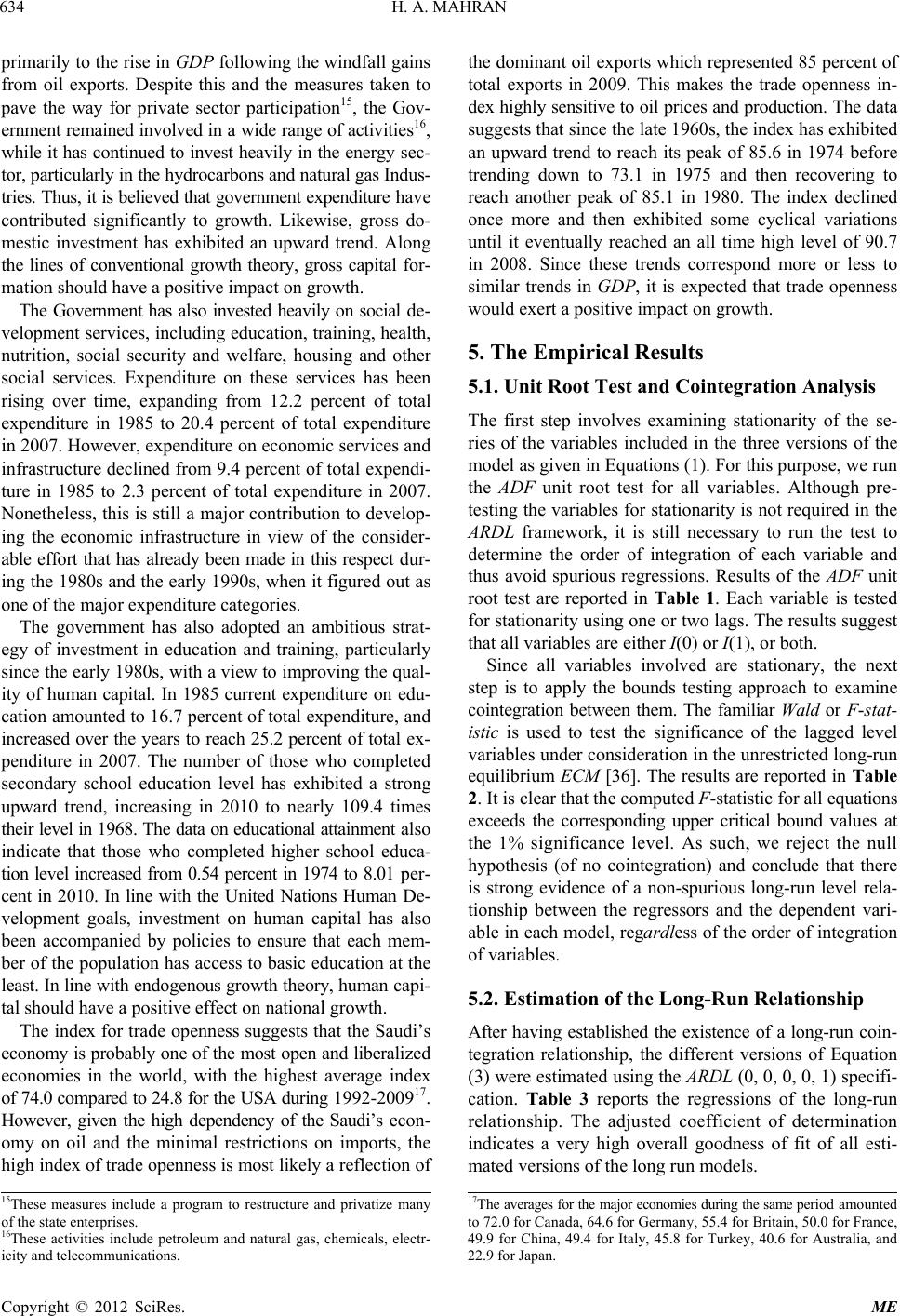

H. A. MAHRAN
634
primarily to the rise in GDP following the windfall gains
from oil exports. Despite this and the measures taken to
pave the way for private sector participation15, the Gov-
ernment remained involved in a wide range of activities16,
while it has continued to invest heavily in the energy sec-
tor, particularly in the hydrocarbons and natural gas Indus-
tries. Thus, it is believed that government expenditure have
contributed significantly to growth. Likewise, gross do-
mestic investment has exhibited an upward trend. Along
the lines of conventional growth theory, gross capital for-
mation should have a positive impact on growth.
The Government has also invested heavily on social de-
velopment services, including education, training, health,
nutrition, social security and welfare, housing and other
social services. Expenditure on these services has been
rising over time, expanding from 12.2 percent of total
expenditure in 1985 to 20.4 percent of total expenditure
in 2007. However, expenditure on economic services and
infrastructure declined from 9.4 percent of total expendi-
ture in 1985 to 2.3 percent of total expenditure in 2007.
Nonetheless, this is still a major contribution to develop-
ing the economic infrastructure in view of the consider-
able effort that has already been made in this respect dur-
ing the 1980s and the early 1990s, when it figured out as
one of the major expenditure categories.
The government has also adopted an ambitious strat-
egy of investment in education and training, particularly
since the early 1980s, with a view to improving the qual-
ity of human capital. In 1985 current expenditure on edu-
cation amounted to 16.7 percent of total expenditure, and
increased over the years to reach 25.2 percent of total ex-
penditure in 2007. The number of those who completed
secondary school education level has exhibited a strong
upward trend, increasing in 2010 to nearly 109.4 times
their level in 1968. The data on educational attainment also
indicate that those who completed higher school educa-
tion level increased from 0.54 percent in 1974 to 8.01 per-
cent in 2010. In line with the United Nations Human De-
velopment goals, investment on human capital has also
been accompanied by policies to ensure that each mem-
ber of the population has access to basic education at the
least. In line with endogenous growth theory, human capi-
tal should have a positive effect on national growth.
The index for trade openness suggests that the Saudi’s
economy is probably one of the most open and liberalized
economies in the world, with the highest average index
of 74.0 compared to 24.8 for the USA during 1992-200917.
However, given the high dependency of the Saudi’s econ-
omy on oil and the minimal restrictions on imports, the
high index of trade openness is most likely a reflection of
the dominant oil exports which represented 85 percent of
total exports in 2009. This makes the trade openness in-
dex highly sensitive to oil prices and production. The data
suggests that since the late 1960s, the index has exhibited
an upward trend to reach its peak of 85.6 in 1974 before
trending down to 73.1 in 1975 and then recovering to
reach another peak of 85.1 in 1980. The index declined
once more and then exhibited some cyclical variations
until it eventually reached an all time high level of 90.7
in 2008. Since these trends correspond more or less to
similar trends in GDP, it is expected that trade openness
would exert a positive impact on growth.
5. The Empirical Results
5.1. Unit Root Test and Cointegration Analysis
The first step involves examining stationarity of the se-
ries of the variables included in the three versions of the
model as given in Equations (1). For this purpose, we run
the ADF unit root test for all variables. Although pre-
testing the variables for stationarity is not required in the
ARDL framework, it is still necessary to run the test to
determine the order of integration of each variable and
thus avoid spurious regressions. Results of the ADF unit
root test are reported in Table 1. Each variable is tested
for stationarity using one or two lags. The results suggest
that all variables are either I(0) or I(1), or both.
Since all variables involved are stationary, the next
step is to apply the bounds testing approach to examine
cointegration between them. The familiar Wald or F-stat-
istic is used to test the significance of the lagged level
variables under consideration in the unrestricted long-run
equilibrium ECM [36]. The results are reported in Table
2. It is clear that the computed F-statistic for all equations
exceeds the corresponding upper critical bound values at
the 1% significance level. As such, we reject the null
hypothesis (of no cointegration) and conclude that there
is strong evidence of a non-spurious long-run level rela-
tionship between the regressors and the dependent vari-
able in each model, regardless of the order of integration
of variables.
5.2. Estimation of the Long-Run Relationship
After having established the existence of a long-run coin-
tegration relationship, the different versions of Equation
(3) were estimated using the ARDL (0, 0, 0, 0, 1) specifi-
cation. Table 3 reports the regressions of the long-run
relationship. The adjusted coefficient of determination
indicates a very high overall goodness of fit of all esti-
mated versions of the long run models.
15These measures include a program to restructure and privatize many
of the state enterprises.
16These activities include petroleum and natural gas, chemicals, electr-
icity and telecommunications.
17The averages for the major economies during the same period amounted
to 72.0 for Canada, 64.6 for Germany, 55.4 for Britain, 50.0 for France,
49.9 for China, 49.4 for Italy, 45.8 for Turkey, 40.6 for Australia, and
22.9 for Japan.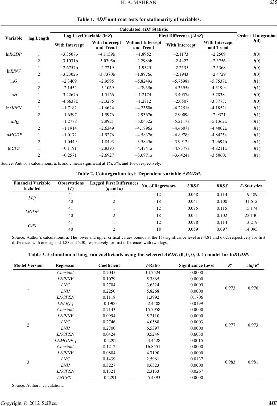

H. A. MAHRAN
635
Table 1. ADF unit root tests for stationarity of variables.
Calculated ADF Statistic
Log Level Variable (lnZ) First Difference (∆lnZ)
Variable lag Length
With Intercept With Intercept
and Trend
Without Intercept
and Trend With InterceptWith Intercept and Trend
Order of Integration
I(d)
lnRGDP 1 –3.3508b –4.1159b –1.8952 –2.1173 –2.2509 I(0)
2 –3.1031b –5.0795a –2.2986b –2.4422 –2.3756 I(0)
1 –2.6757b –2.7219 –1.9325 –2.2535 –2.5368 I(0)
lnRINV 2 –3.2302b –3.7370b –1.8976c –2.1943 –2.4729 I(0)
lnG 1 –2.3409 –2.9595 –5.8249a –5.7598a –5.7537a I(1)
2 –2.1452 –3.1069 –4.3935a –4.3395a –4.3199a I(1)
lnH 1 –3.4267b –1.5166 –1.2174 –3.4057a –5.7838a I(0)
2 –4.6638a –2.3285 –1.2712 –2.0507 –3.3773c I(0)
lnOPEN 1 –1.7182 –1.6624 –4.2350a –4.2251a –4.1852a I(1)
2 –1.6597 –1.5976 –2.9367a –2.9009c –2.9321 I(1)
lnLIQ 1 –1.2778 –2.8921 –5.0432a –5.2117a –5.1362a I(1)
2 –1.1914 –2.6349 –4.1896a –4.4607a –4.4002a I(1)
lnMGDP 1 –1.0172 –1.9276 –4.5837a –4.8978a –4.8425a I(1)
2 –1.0449 –1.8493 –3.5845a –3.9912a –3.9694b I(1)
lnCPS 1 –0.1191 –2.8393 –4.4741a –4.8377a –4.8211a I(1)
2 –0.2571 –2.6927 –3.0971a –3.6424a –3.5060c I(1)
Source: Author’s calculations. a, b, and c mean significant at 1%, 5%, and 10%, respectively.
Table 2. Cointegration test: Dependent variable ∆RGDP.
Financial Variable
Included
Observations
(T)
Lagged First Differences
(q and k) No. of RegressorsURSS RRSS F-Statistica
41 1 12 0.068 0.114 19.489
LIQ 40 2 18 0.041 0.100 31.612
41 1 12 0.075 0.115 15.174
MGDP 40 2 18 0.051 0.102 22.130
41 1 12 0.078 0.114 13.219
CPS 40 2 18 0.059 0.097 14.095
Source: Author’s calculations. a. The lower and upper critical values bounds at the 1% significance level are 4.81 and 6.02, respectively for first
differences with one lag and 3.88 and 5.30, respectively for first differences with two lags.
Table 3. Estimation of long-run coefficients using the selected ARDL (0, 0, 0, 0, 1) model for lnRGDP.
Model Version Regressor Coefficient t-Ratio Significance Level R2 Adj R2
Constant 8.7045 14.7524 0.0000
LNRINV 0.1079 5.3865 0.0000
LNG 0.2704 3.6324 0.0009
LNH 0.2250 5.8268 0.0000
LNOPEN 0.1118 1.3992 0.1706
1
LNLIQ–1 –0.1900 –2.4408 0.0199
0.973 0.970
Constant 8.7143 15.7958 0.0000
LNRINV 0.0994 5.2110 0.0000
LNG 0.2746 4.0588 0.0003
LNH 0.2700 6.5397 0.0000
LNOPEN 0.0424 0.5249 0.6030
2
LNMGDP–1 –0.2292 –3.4428 0.0015
0.977 0.973
Constant 8.1212 16.8551 0.0000
LNRINV 0.0804 4.7190 0.0000
LNG 0.1439 2.5961 0.0137
LNH 0.3227 8.6523 0.0000
LNOPEN 0.1321 2.3133 0.0267
3
LNCPS–1 –0.2291 –5.4393 0.0000
0.983 0.981
Source: Authors’ calculations.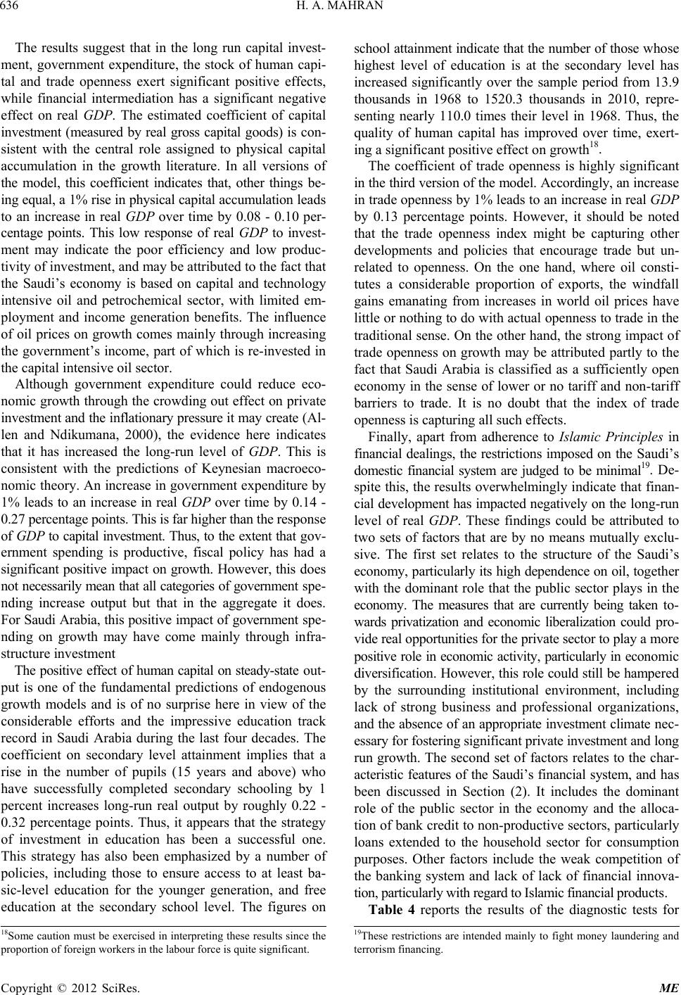

H. A. MAHRAN
636
The results suggest that in the long run capital invest-
ment, government expenditure, the stock of human capi-
tal and trade openness exert significant positive effects,
while financial intermediation has a significant negative
effect on real GDP. The estimated coefficient of capital
investment (measured by real gross capital goods) is con-
sistent with the central role assigned to physical capital
accumulation in the growth literature. In all versions of
the model, this coefficient indicates that, other things be-
ing equal, a 1% rise in physical capital accumulation leads
to an increase in real GDP over time by 0.08 - 0.10 per-
centage points. This low response of real GDP to invest-
ment may indicate the poor efficiency and low produc-
tivity of investment, and may be attributed to the fact that
the Saudi’s economy is based on capital and technology
intensive oil and petrochemical sector, with limited em-
ployment and income generation benefits. The influence
of oil prices on growth comes mainly through increasing
the government’s income, part of which is re-invested in
the capital intensive oil sector.
Although government expenditure could reduce eco-
nomic growth through the crowding out effect on private
investment and the inflationary pressure it may create (Al-
len and Ndikumana, 2000), the evidence here indicates
that it has increased the long-run level of GDP. This is
consistent with the predictions of Keynesian macroeco-
nomic theory. An increase in government expenditure by
1% leads to an increase in real GDP over time by 0.14 -
0.27 percentage points. This is far higher than the response
of GDP to capital investment. Thus, to the extent that gov-
ernment spending is productive, fiscal policy has had a
significant positive impact on growth. However, this does
not necessarily mean that all categories of government spe-
nding increase output but that in the aggregate it does.
For Saudi Arabia, this positive impact of government spe-
nding on growth may have come mainly through infra-
structure investment
The positive effect of human capital on steady-state out-
put is one of the fundamental predictions of endogenous
growth models and is of no surprise here in view of the
considerable efforts and the impressive education track
record in Saudi Arabia during the last four decades. The
coefficient on secondary level attainment implies that a
rise in the number of pupils (15 years and above) who
have successfully completed secondary schooling by 1
percent increases long-run real output by roughly 0.22 -
0.32 percentage points. Thus, it appears that the strategy
of investment in education has been a successful one.
This strategy has also been emphasized by a number of
policies, including those to ensure access to at least ba-
sic-level education for the younger generation, and free
education at the secondary school level. The figures on
school attainment indicate that the number of those whose
highest level of education is at the secondary level has
increased significantly over the sample period from 13.9
thousands in 1968 to 1520.3 thousands in 2010, repre-
senting nearly 110.0 times their level in 1968. Thus, the
quality of human capital has improved over time, exert-
ing a significant positive effect on growth18.
The coefficient of trade openness is highly significant
in the third version of the model. Accordingly, an increase
in trade openness by 1% leads to an increase in real GDP
by 0.13 percentage points. However, it should be noted
that the trade openness index might be capturing other
developments and policies that encourage trade but un-
related to openness. On the one hand, where oil consti-
tutes a considerable proportion of exports, the windfall
gains emanating from increases in world oil prices have
little or nothing to do with actual openness to trade in the
traditional sense. On the other hand, the strong impact of
trade openness on growth may be attributed partly to the
fact that Saudi Arabia is classified as a sufficiently open
economy in the sense of lower or no tariff and non-tariff
barriers to trade. It is no doubt that the index of trade
openness is capturing all such effects.
Finally, apart from adherence to Islamic Principles in
financial dealings, the restrictions imposed on the Saudi’s
domestic financial system are judged to be minimal19. De-
spite this, the results overwhelmingly indicate that finan-
cial development has impacted negatively on the long-run
level of real GDP. These findings could be attributed to
two sets of factors that are by no means mutually exclu-
sive. The first set relates to the structure of the Saudi’s
economy, particularly its high dependence on oil, together
with the dominant role that the public sector plays in the
economy. The measures that are currently being taken to-
wards privatization and economic liberalization could pro-
vide real opportunities for the private sector to play a more
positive role in economic activity, particularly in economic
diversification. However, this role could still be hampered
by the surrounding institutional environment, including
lack of strong business and professional organizations,
and the absence of an appropriate investment climate nec-
essary for fostering significant private investment and long
run growth. The second set of factors relates to the char-
acteristic features of the Saudi’s financial system, and has
been discussed in Section (2). It includes the dominant
role of the public sector in the economy and the alloca-
tion of bank credit to non-productive sectors, particularly
loans extended to the household sector for consumption
purposes. Other factors include the weak competition of
the banking system and lack of lack of financial innova-
tion, particularly with regard to Islamic financial products.
Table 4 reports the results of the diagnostic tests for
18Some caution must be exercised in interpreting these results since the
p
roportion of foreign workers in the labour force is quite significant.
19These restrictions are intended mainly to fight money laundering and
terrorism financing.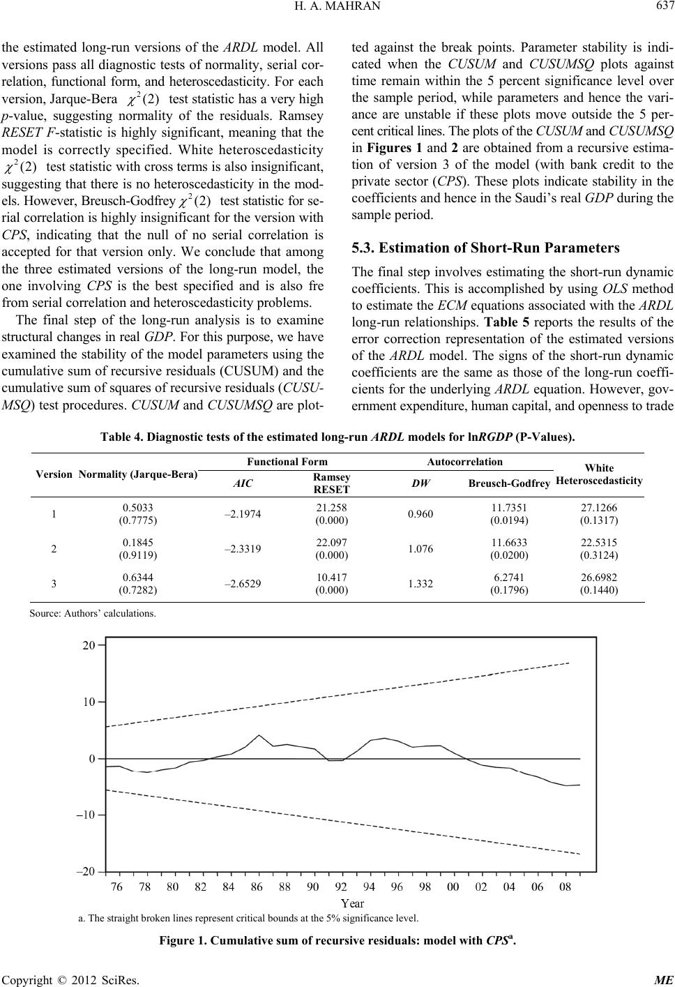

H. A. MAHRAN 637
the estimated long-run versions of the ARDL model. All
versions pass all diagnostic tests of normality, serial cor-
relation, functional form, and heteroscedasticity. For each
version, Jarque-Bera test statistic has a very high
p-value, suggesting normality of the residuals. Ramsey
RESET F-statistic is highly significant, meaning that the
model is correctly specified. White heteroscedasticity
test statistic with cross terms is also insignificant,
suggesting that there is no heteroscedasticity in the mod-
els. However, Breusch-Godfrey test statistic for se-
rial correlation is highly insignificant for the version with
CPS, indicating that the null of no serial correlation is
accepted for that version only. We conclude that among
the three estimated versions of the long-run model, the
one involving CPS is the best specified and is also fre
from serial correlation and heteroscedasticity problems.
2(2)

2(2)

2(2)

The final step of the long-run analysis is to examine
structural changes in real GDP. For this purpose, we have
examined the stability of the model parameters using the
cumulative sum of recursive residuals (CUSUM) and the
cumulative sum of squares of recursive residuals (C USU-
MSQ) test procedures. CUSUM and CUSUMSQ are plot-
ted against the break points. Parameter stability is indi-
cated when the CUSUM and CUSUMSQ plots against
time remain within the 5 percent significance level over
the sample period, while parameters and hence the vari-
ance are unstable if these plots move outside the 5 per-
cent critical lines. The plots of the CUSUM and CUS UMSQ
in Figures 1 and 2 are obtained from a recursive estima-
tion of version 3 of the model (with bank credit to the
private sector (CPS). These plots indicate stability in the
coefficients and hence in the Saudi’s real GDP during the
sample period.
5.3. Estimation of Short-Run Parameters
The final step involves estimating the short-run dynamic
coefficients. This is accomplished by using OLS method
to estimate the ECM equations associated with the ARDL
long-run relationships. Table 5 reports the results of the
error correction representation of the estimated versions
of the ARDL model. The signs of the short-run dynamic
coefficients are the same as those of the long-run coeffi-
cients for the underlying ARDL equation. However, gov-
ernment expenditure, human capital, and openness to trade
Table 4. Diagnostic tests of the estimated long-run ARDL models for lnRGDP (P-Values).
Functional Form Autocorrelation
Version Normality (Jarque-Bera) AIC Ramsey
RESET DW Breusch-Godfrey
White
Heteroscedasticity
1 0.5033
(0.7775) –2.1974 21.258 (0.000) 0.960 11.7351 (0.0194)
27.1266
(0.1317)
2 0.1845
(0.9119) –2.3319 22.097 (0.000) 1.076 11.6633 (0.0200)
22.5315
(0.3124)
3 0.6344
(0.7282) –2.6529 10.417 (0.000) 1.332 6.2741 (0.1796)
26.6982
(0.1440)
Source: Authors’ calculations.
a. The straight broken lines represent critical bounds at the 5% significance level.
Figure 1. Cumulative sum of recursive residuals: model with CPSa.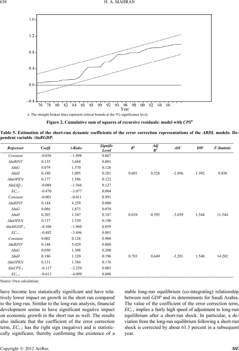

H. A. MAHRAN
638
a. The straight broken lines represent critical bounds at the 5% significance level.
Figure 2. Cumulative sum of squares of recursive residuals: model with CPSa
Table 5. Estimation of the short-run dynamic coefficients of the error correction representations of the ARDL models: De-
pendent variable ∆lnRGDP.
Regressor Coeff. t-Ratio Signific
Level R2 Adj R2 AIC DW F-Statistic
Constant –0.036 –1.898 0.067
∆lnRINV 0.135 3.684 0.001
∆lnG 0.079 1.570 0.126
∆lnH 0.180 1.095 0.281
∆lnOPEN 0.177 1.586 0.122
∆lnLIQ–1 –0.088 –1.566 0.127
ECt–1 –0.470 –3.077 0.004
0.601 0.528 –2.896 1.392 9.038
Constant –0.001 –0.011 0.991
∆lnRINV 0.144 4.259 0.000
∆lnG 0.086 1.873 0.070
∆lnH 0.203 1.347 0.187
∆lnOPEN 0.137 1.339 0.190
∆lnMGDP–1 –0.106 –1.960 0.059
ECt–1 –0.492 –3.496 0.001
0.658 0.595 –3.059 1.544 11.544
Constant 0.002 0.126 0.900
∆lnRINV 0.148 5.029 0.000
∆lnG 0.050 1.308 0.200
∆lnH 0.186 1.320 0.196
∆lnOPEN 0.131 1.384 0.176
∆lnCPS–1 –0.117 –3.259 0.003
ECt–1 –0.613 –4.099 0.000
0.703 0.649 –3.201 1.548 14.202
Source: Own calculations.
have become less statistically significant and have rela-
tively lower impact on growth in the short run compared
to the long-run. Similar to the long-run analysis, financial
development seems to have significant negative impact
on economic growth in the short run as well. The results
also indicate that the coefficient of the error correction
term, ECt–1 has the right sign (negative) and is statistic-
cally significant, thereby confirming the existence of a
stable long-run equilibrium (co-integrating) relationship
between real GDP and its determinants for Saudi Arabia.
The value of the coefficient of the error correction term,
ECt–1 implies a fairly high speed of adjustment to long-run
equilibrium after a short-run shock. In particular, a de-
viation from the long-run equilibrium following a short-run
shock is corrected by about 61.3 percent in a subsequent
year.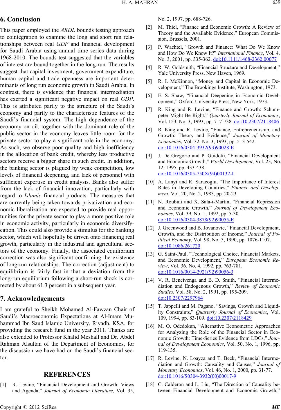

H. A. MAHRAN 639
6. Conclusion
This paper employed the ARDL bounds testing approach
to cointegration to examine the long and short run rela-
tionships between real GDP and financial development
for Saudi Arabia using annual time series data during
1968-2010. The bounds test suggested that the variables
of interest are bound together in the long-run. The results
suggest that capital investment, government expenditure,
human capital and trade openness are important deter-
minants of long run economic growth in Saudi Arabia. In
contrast, there is evidence that financial intermediation
has exerted a significant negative impact on real GDP.
This is attributed partly to the structure of the Saudi’s
economy and partly to the characteristic features of the
Saudi’s financial system. The high dependence of the
economy on oil, together with the dominant role of the
public sector in the economy leaves little room for the
private sector to play a significant role in the economy.
As such, we observe poor quality and high inefficiency
in the allocation of bank credit, whereby less productive
sectors receive a bigger share in such credit. In addition,
the banking sector is plagued by weak competition, low
levels of financial deepening, and lack of personnel with
sufficient expertise in credit analysis. Banks also suffer
from the lack of financial innovation, particularly with
regard to Islamic financial products. The measures that
are currently being taken towards privatization and eco-
nomic liberalization are expected to provide real oppor-
tunities for the private sector to play a more positive role
in economic activity, particularly in economic diversify-
cation. This could also provide a stimulus for the banking
sector, which will hopefully be driven onto financing real
growth, particularly in the industrial and agricultural sec-
tors of the economy. Finally, the associated equilibrium
correction was also significant confirming the existence
of long-run relationships. The correction (adjustment) to
equilibrium is fairly fast in that a deviation from the
long-run equilibrium following a short-run shock is cor-
rected by about 61.3 percent in a subsequent year.
7. Acknowledgements
I am grateful to Sheikh Mohamed Al-Fawzan Chair of
Saudi’s Macroeconomic Expectations at Al-Imam Mu-
hammad Ibn Saud Islamic University, Riyadh, KSA, for
providing the research fund in the year 2011. Thanks are
also extended to Professor Khalid Meshall and Dr. Abdel
Rahman Alsultan of the Department of Economics, for
the discussion we have had on the Saudi’s financial sec-
tor.
REFERENCES
[1] R. Levine, “Financial Development and Growth: Views
and Agenda,” Journal of Economic Literature, Vol. 35,
No. 2, 1997, pp. 688-726.
[2] M. Thiel, “Finance and Economic Growth: A Review of
Theory and the Available Evidence,” European Commis-
sion, Brussels, 2001.
[3] P. Wachtel, “Growth and Finance: What Do We Know
and How Do We Know It?” International Finance, Vol. 4,
No. 3, 2001, pp. 335-362. doi:10.1111/1468-2362.00077
[4] R. W. Goldsmith, “Financial Structure and Development,”
Yale University Press, New Haven, 1969.
[5] R. I. McKinnon, “Money and Capital in Economic De-
velopment,” The Brookings Institute, Washington, 1973.
[6] E. S. Shaw, “Financial Deepening in Economic Devel-
opment,” Oxford University Press, New York, 1973.
[7] R. King and R. Levine, “Finance and Growth: Schum-
peter Might Be Right,” Quarterly Journal of Economics,
Vol. 153, No. 3, 1993, pp. 717-738. doi:10.2307/2118406
[8] R. King and R. Levine, “Finance, Entrepreneurship, and
Growth: Theory and Evidence,” Journal of Monetary
Economics, Vol. 32, No. 3, 1993, pp. 513-542.
doi:10.1016/0304-3932(93)90028-E
[9] J. De Gregorio and P. Guidotti, “Financial Development
and Economic Growth,” World Development, Vol. 23, No.
12, 1995, pp. 433-438.
doi:10.1016/0305-750X(94)00132-I
[10] A. Lanyi and R. Saracoglu, “The Importance of Interest
Rates in Developing Countries,” Finance and Develop-
ment, Vol. 20, No. 2, 1983, pp. 20-23.
[11] N. Roubini and X. Sala-i-Martin, “Financial Repression
and Economic Growth,” Journal of Development Eco-
nomics, Vol. 39, No. 1, 1992, pp. 5-30.
doi:10.1016/0304-3878(92)90055-E
[12] J. Greenwood and B. Jovanovic, “Financial Development,
Growth, and the Distribution of Income,” Journal of Po-
litical Economy, Vol. 98, No. 5, 1990, pp. 1076-1107.
doi:10.1086/261720
[13] G. Saint-Paul, “Technological Choice, Financial Markets,
and Economic Development,” European Economic Re-
view, Vol. 36, No. 4, 1992, pp. 763-781.
doi:10.1016/0014-2921(92)90056-3
[14] V. R. Bencivenga and B. D. Smith, “Financial Interme-
diation and Endogenous Growth,” Review of Economic
Studies, Vol. 58, No. 2, 1991, pp. 195-209.
doi:10.2307/2297964
[15] T. Jappelli and M. Pagano, “Savings, Growth and Liquid-
ity Constraints,” Quarterly Journal of Economics, Vol.
109, 1994, pp. 83-109. doi:10.2307/2118429
[16] M. O. Odedokun, “Alternative Econometric Approaches
for Analyzing the Role of the Financial Sector in Eco-
nomic Growth: Time-Series Evidence from LDCs,” Jour-
nal of Development Economics, Vol. 50, No. 1, 1996, pp.
119-135.
[17] R. Levine, N. Loayza and T. Beck, “Financial Interme-
diation and Growth: Causality and Causes,” Journal of
Monetary Ec onomics, Vol. 46, No. 1, 2000, pp. 31-77.
doi:10.1016/S0304-3932(00)00017-9
[18] C. Calderon and L. Liu, “The Direction of Causality be-
tween Financial Development and Economic Growth,”

H. A. MAHRAN
640
Journal of Development Economics, Vol. 72, No. 1, 2003,
pp. 321-334.
[19] D. K. Christopoulos and E. G. Tsionas, “Financial De-
velopment and Economic Growth: Evidence from Panel
Unit Root and Cointegration Tests,” Journal of Develop-
ment Economics, Vol. 73, No. 1, 2004, pp. 55-74.
doi:10.1016/j.jdeveco.2003.03.002
[20] S. C. Valverde, R. L. del Paso and F. R. Fernández,
“Banks, Financial Innovations and Regional Growth,”
Working Paper No. 04-34, Department of Economics,
University of Granada, Granada, 2004.
[21] J. Z. Shan, “Does Financial Development ‘Lead’ Econo-
mic Growth? A Vector Auto-Regression Appraisal,” Ap-
plied Economics, Vol. 37, No. 12, 2005, pp. 1353-1367.
doi:10.1080/00036840500118762
[22] H. Zang and Y. C. Kim, “Does Financial Development
Precede Growth? Robinson and Lucas Might Be Right,”
Applied Economic Letters, Vol. 14, No. 1, 2007, pp. 15-
19. doi:10.1080/13504850500425469
[23] J. E. U. Ndebbio, “Financial Deepening, Economic Growth
and Development: Evidence from Selected Sub-Saharan
African Countries,” AERC Research Paper 142, Nairobi,
2004.
[24] S. Abu-Bader and A. Abu-Qarn, “Financial Development
and Economic Growth: The Egyptian Experience,” Jour-
nal of Policy Modeling, Vol. 30, No. 4, 2008, pp. 887-898.
doi:10.1016/j.jpolmod.2007.02.001
[25] S. E. Mohamed and M. Sidiropoulos, “Finance-Growth
Nexus in Sudan: Empirical Assessment Based on an Ap-
plication of the Autoregressive Distributed Lag (ARDL)
Model,” Working Paper, BETA-Theme, University of
Strasbourg, 2006.
[26] A. Al-Hassan, M. Khamis and N. Oulidi, “The GCC
Banking Sector: Topography and Analysis,” IMF Work-
ing Paper No. WP/10/87, International Monetary Fund,
Washington DC, 2010.
[27] Saudi Arabian Monetary Authority, Forty Sixth Annual
Report, Riyadh, 2010.
[28] R. T. Ariss, R. Rezvanian and S. M. Mehdian, “Cost Effi-
ciency, Technological Progress and Productivity Growth
of Banks in GCC Countries,” International Journal of
Business, Vol. 12, No. 4, 2007, pp. 471-487.
[29] D. S. Allen and L. Ndikumana, “Financial Intermediation
and Economic Growth in Southern Africa,” Federal Re-
serve Bank of St. Louis, Working Paper 1998-004B,
1998.
[30] P. L. Rousseau and P. Wachtel, “Financial Intermediation
and Economic Performance: Historical Evidence from
Industrial Countries,” Journal of Money, Credit, and Bank-
ing, Vol. 30, No. 4, 1998, pp. 657-678.
doi:10.2307/2601123
[31] T. Beck, A. Demirguc-Kunt, R. Levine and V. Maksi-
movic, “Financial Structure and Economic Development:
Firm, Industry, and Country Evidence,” World Bank
Working Paper No. 2423, 2000.
[32] World Bank, “Finance for Growth,” World Bank, Wash-
ington DC, 2001.
[33] R. Levine and S. Zervos, “Stock Markets, Banks, and
Economic Growth,” American Economic Review, Vol. 88,
No. 3, 1998, pp. 537-558.
[34] R. Levine and D. Renelt, “A Sensitivity Analysis of
Cross-Country Growth Regressions,” American Eco-
nomic Review, Vol. 82, No. 4, 1992, pp. 942-963.
[35] W. R. Easterly and S. Rebelo, “Fiscal Policy and Eco-
nomic Growth: An Empirical Investigation,” Journal of
Monetary Economics, Vol. 32, No. 3, 1993, pp. 417-457.
doi:10.1016/0304-3932(93)90025-B
[36] S. Fischer, “The Role of Macroeconomic Factors in
Growth,” Journal of Monetary Economics, Vol. 32, No. 3,
1993, pp. 485-512.
[37] M. H. Pesaran, Y. Shin and R. J. Smith, “Bounds Testing
Approaches to the Analysis of Level Relationships,”
Journal of Applied Econometrics, Vol. 16, No. 3, 2001,
pp. 289-326. doi:10.1002/jae.616
[38] M. H. Pesaran and Y. Shin, “An Autoregressive Distrib-
uted Lag Modeling Approach to Cointegration, Chapter
11, in Econometrics and Economic Theory in the 20th
Century,” The Ragnar Frisch Centennial Symposium,
Cambridge University Press, 1999.
[39] M. H. Pesaran and R. J. Smith, “Estimating Long-Run
Relationships from Dynamic Heterogeneous Panels,”
Journal of Econometrics, Vol. 68, No. 1, 1995, pp. 79-
113. doi:10.1016/0304-4076(94)01644-F
[40] R. F. Engle and C. W. J. Granger, “Co-Integration and
Error Correction: Representation, Estimation and Test-
ing,” Econometrica, Vol. 55, No. 2, 1987, pp. 251-276.
doi:10.2307/1913236
[41] S. Johansen, “Statistical Analysis of Cointegrating Vec-
tors,” Journal of Economic Dynamics and Control, Vol.
12, No. 2-3, 1988, pp. 231-254.
doi:10.1016/0165-1889(88)90041-3
[42] S. Johansen and K. Juselius, “Maximum Likelihood Es-
timation and Inference on Cointegration with Application
to the Demand for Money,” Oxford Bulletin of Economics
and Statistics, Vol. 52, No. 2, 1990, pp. 169-210.
doi:10.1111/j.1468-0084.1990.mp52002003.x
[43] M. H. Pesaran and B. Pesaran, “Working with Microfit 4.0:
Interactive Econometric Analysis,” Oxford University
Press, Oxford, 1997.