The Asset Pricing System

doi:10.4236/me.2012.35062

Paper Menu >>

Journal Menu >>

Modern Economy, 2012, 3, 473-480

http://dx.doi.org/10.4236/me.2012.35062 Published Online September 2012 (http://www.SciRP.org/journal/me)

The Asset Pricing System

Yi-Jang Yu

Department of Economics, Ming Chuan University, Taipei, Chinese Taipei

Email: yjyu@mail.mcu.edu.tw

Received May 5, 2012; revised June 6, 2012; accepted June 15, 2012

ABSTRACT

Mainstream asset pricing models are all inappropriate when they consistently insist on applying one single model to

deal with a reality filled with different aspects of asset pricing. In addition, those models also treat the right environment

variable too lightly hence can not rightly do the job of asset pricing. In this study, based on the portfolio theory and the

principle of supply and demand, a more reasonable asset pricing system including five different models will be sug-

gested to provide a necessary function of automatic price stabilization and to better serve our financial market.

Keywords: Asset Pricing System; Environment Variable; Portfolio Theory; Automatic Price Stabilization

1. Introduction

Since the mainstream asset pricing models can not restrain

themselves from generating price bubbles in the financial

market (Summers, 1985 [1]; Krugman, 2009 [2]; Colan-

der, 2010 [3]), they certainly deserve our closer attention.

In recent years, final conclusions regarding the major

causes of recent financial crises still focus on market con-

straints such as loose controls over financial derivatives

or credit or monetary policies (Kindleberger, 2005 [4];

Askari et al., 2010 [5]; Bresser-Pereira, 2010 [6]). How-

ever, if those mainstream asset pricing models can not be

tamed by nature, then unleashing their constraints would

only further exaggerate their power of sabotage.

Equally important is that, when asset risk and return

can only be endogenously determined and both are of much

concern to investors, clearly it is impossible to apply just

one single model to price assets, not to mention that there

are still other considerations including the separation be-

tween normative and positive analyses needing to be

taken care of. In reality, we have no choice but to apply a

system instead of one single model to manage the job of

asset pricing.

The main tasks of this study are therefore twofold. The

first is to point out that mainstream asset pricing models

are all inappropriate when they consistently insist on

applying one single model to deal with a reality filled

with different aspects of asset pricing. Accordingly, the

second task of this study is to suggest a necessary asset

pricing system which, by its own properties, can provide

a safer ground to serve our financial market.

1.1. Literature Review

Within the econometric approaches to asset pricing, strictly

using only company variables emerged earlier, and the

MM theorem proposed by Miller and Modigliani in 1961

was deemed to be the pioneering study in this field (Chen

and Zhang, 2007 [7]). By contrast, Fama (1981) [8] started

to lay the econometric foundation between asset price

variation and macroeconomic variables including GDP,

monetary supply and other related variables. Not surpris-

ingly, combining both microeconomic and macroeconomic

variables into one econometric model also attracted some

attention (Lev and Thiagarajan, 1993 [9]; Swanson et al.,

2003 [10]). However, when the set of explanatory variables

with the best explanatory power could not be standard-

ized for different individual assets, requiring more weights

to be put on company variables, or asset portfolios, re-

quiring more weights to be attached to macroeconomic

variables, there was no end to the disputes that arose.

As to those asset pricing models constructed with

theoretical foundations, the first category featured the

return aspect and was described by Graham and Dodd in

1934, later becoming the Dividend Discount Model pro-

posed by Gordon and Shapiro in 1956 (Bettman et al.,

2009 [11]). After that, two more kindred products of the

Earnings Capitalization Model and the Residual Income

Valuation Model had also been suggested (Kothari, 2001

[12]). The problem is, as long as all of them have to ap-

ply time series corporate net incomes to forecast the net

income in the next period, they can easily become econo-

metric models (Collins and Kothari, 1989 [13]; Dechow

et al., 1999 [14]). The second category can be classified

as risk evaluation models, and the CAPM is clearly the

most important representative. The scale of its family is

still growing up to these days. While some consistently

oppose it (Fama and French, 1996 [15]; 2004 [16]), some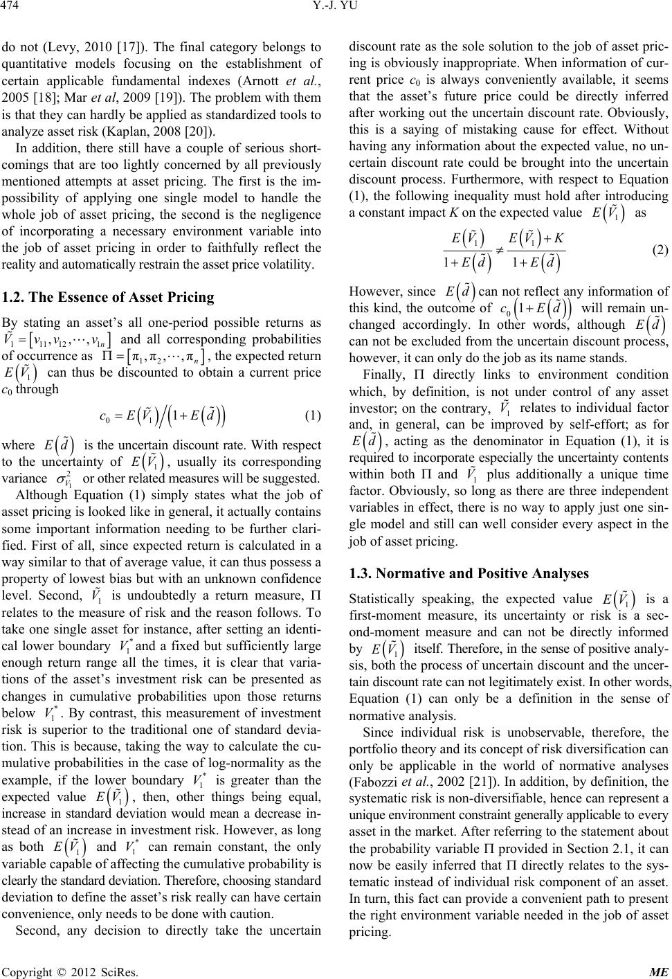

Y.-J. YU

474

do not (Levy, 2010 [17]). The final category belongs to

quantitative models focusing on the establishment of

certain applicable fundamental indexes (Arnott et al.,

2005 [18]; Mar et al, 2009 [19]). The problem with them

is that they can hardly be applied as standardized tools to

analyze asset risk (Kaplan, 2008 [20]).

In addition, there still have a couple of serious short-

comings that are too lightly concerned by all previously

mentioned attempts at asset pricing. The first is the im-

possibility of applying one single model to handle the

whole job of asset pricing, the second is the negligence

of incorporating a necessary environment variable into

the job of asset pricing in order to faithfully reflect the

reality and automatically restrain the asset price volatility.

1.2. The Essence of Asset Pricing

By stating an asset’s all one-period possible returns as





Vv



112 and all corresponding probabilities

of occurrence as



,,,v v



12 n, the expected return

can thus be discounted to obtain a current price

c0 through

π,π,,π















cE

1V Ed











(1)

where is the uncertain discount rate. With respect

to the uncertainty of 1, usually its corresponding

variance 1



or other related measures will be suggested.

Although Equation (1) simply states what the job of

asset pricing is looked like in general, it actually contains

some important information needing to be further clari-

fied. First of all, since expected return is calculated in a

way similar to that of average value, it can thus possess a

property of lowest bias but with an unknown confidence

level. Second, 1 is undoubtedly a return measure, 

relates to the measure of risk and the reason follows. To

take one single asset for instance, after setting an identi-

cal lower boundary 1and a fixed but sufficiently large

enough return range all the times, it is clear that varia-

tions of the asset’s investment risk can be presented as

changes in cumulative probabilities upon those returns

below . By contrast, this measurement of investment

risk is superior to the traditional one of standard devia-

tion. This is because, taking the way to calculate the cu-

mulative probabilities in the case of log-normality as the

example, if the lower boundary 1 is greater than the

expected value , then, other things being equal,

increase in standard deviation would mean a decrease in-

stead of an increase in investment risk. However, as long

as both 1 and 1

V can remain constant, the only

variable capable of affecting the cumulative probability is

clearly the standard deviation. Therefore, choosing standard

deviation to define the asset’s risk really can have certain

convenience, only needs to be done with caution.





*









Second, any decision to directly take the uncertain

discount rate as the sole solution to the job of asset pric-

ing is obviously inappropriate. When information of cur-

rent price c0 is always conveniently available, it seems

that the asset’s future price could be directly inferred

after working out the uncertain discount rate. Obviously,

this is a saying of mistaking cause for effect. Without

having any information about the expected value, no un-

certain discount rate could be brought into the uncertain

discount process. Furthermore, with respect to Equation

(1), the following inequality must hold after introducing

a constant impact K on the expected value as







EVEV K

Ed Ed









(2)



However, since







1cEd

can not reflect any information of

this kind, the outcome of 0 will remain un-

changed accordingly. In other words, although







can not be excluded from the uncertain discount process,

however, it can only do the job as its name stands.

Finally,  directly links to environment condition

which, by definition, is not under control of any asset

investor; on the contrary, 1 relates to individual factor

and, in general, can be improved by self-effort; as for







, acting as the denominator in Equation (1), it is

required to incorporate especially the uncertainty contents

within both  and 1 plus additionally a unique time

factor. Obviously, so long as there are three independent

variables in effect, there is no way to apply just one sin-

gle model and still can well consider every aspect in the

job of asset pricing.

1.3. Normative and Positive Analyses



Statistically speaking, the expected value





1 is a

first-moment measure, its uncertainty or risk is a sec-

ond-moment measure and can not be directly informed







1 itself. Therefore, in the sense of positive analy-

sis, both the process of uncertain discount and the uncer-

tain discount rate can not legitimately exist. In other words,

Equation (1) can only be a definition in the sense of

normative analysis.

Since individual risk is unobservable, therefore, the

portfolio theory and its concept of risk diversification can

only be applicable in the world of normative analyses

(Fabozzi et al., 2002 [21]). In addition, by definition, the

systematic risk is non-diversifiable, hence can represent a

unique environment constraint generally applicable to every

asset in the market. After referring to the statement about

the probability variable  provided in Section 2.1, it can

now be easily inferred that  directly relates to the sys-

tematic instead of individual risk component of an asset.

In turn, this fact can provide a convenient path to present

the right environment variable needed in the job of asset

pricing.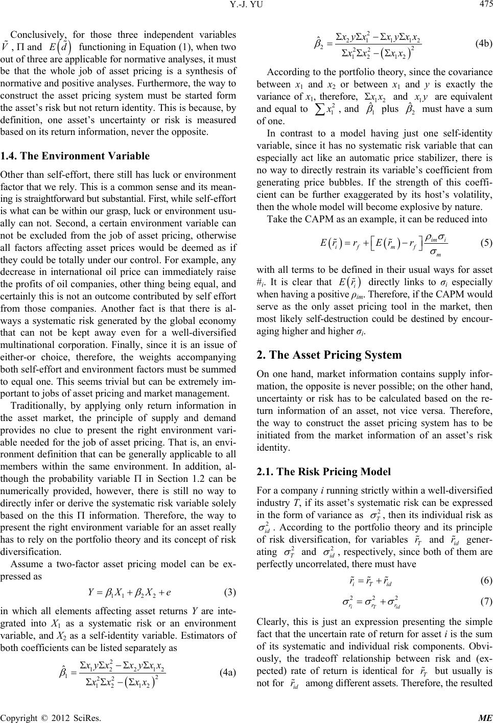

Y.-J. YU 475

Conclusively, for those three independent variables

,  and functioning in Equation (1), when two

out of three are applicable for normative analyses, it must

be that the whole job of asset pricing is a synthesis of

normative and positive analyses. Furthermore, the way to

construct the asset pricing system must be started form

the asset’s risk but not return identity. This is because, by

definition, one asset’s uncertainty or risk is measured

based on its return information, never the opposite.







112 2

1.4. The Environment Variable

Other than self-effort, there still has luck or environment

factor that we rely. This is a common sense and its mean-

ing is straightforward but substantial. First, while self-effort

is what can be within our grasp, luck or environment usu-

ally can not. Second, a certain environment variable can

not be excluded from the job of asset pricing, otherwise

all factors affecting asset prices would be deemed as if

they could be totally under our control. For example, any

decrease in international oil price can immediately raise

the profits of oil companies, other thing being equal, and

certainly this is not an outcome contributed by self effort

from those companies. Another fact is that there is al-

ways a systematic risk generated by the global economy

that can not be kept away even for a well-diversified

multinational corporation. Finally, since it is an issue of

either-or choice, therefore, the weights accompanying

both self-effort and environment factors must be summed

to equal one. This seems trivial but can be extremely im-

portant to jobs of asset pricing and market management.

Traditionally, by applying only return information in

the asset market, the principle of supply and demand

provides no clue to present the right environment vari-

able needed for the job of asset pricing. That is, an envi-

ronment definition that can be generally applicable to all

members within the same environment. In addition, al-

though the probability variable  in Section 1.2 can be

numerically provided, however, there is still no way to

directly infer or derive the systematic risk variable solely

based on the this  information. Therefore, the way to

present the right environment variable for an asset really

has to rely on the portfolio theory and its concept of risk

diversification.

Assume a two-factor asset pricing model can be ex-

pressed as



 



(3)

in which all elements affecting asset returns Y are inte-

grated into X1 as a systematic risk or an environment

variable, and X2 as a self-identity variable. Estimators of

both coefficients can be listed separately as

122

ˆ212







xyxx







(4a)

21 112

12 12

yx xyxx

xx xx





 

(4b)

According to the portfolio theory, since the covariance

between x1 and x2 or between x1 and y is exactly the

variance of x1, therefore, 2



and 1

are equivalent

and equal to 1

ˆ2



, and



plus



must have a sum

of one.

In contrast to a model having just one self-identity

variable, since it has no systematic risk variable that can

especially act like an automatic price stabilizer, there is

no way to directly restrain its variable’s coefficient from

generating price bubbles. If the strength of this coeffi-

cient can be further exaggerated by its host’s volatility,

then the whole model will become explosive by nature.

Take the CAPM as an example, it can be reduced into

 

im i

if mf

Er rErr







 



 (5)

with all terms to be defined in their usual ways for asset

#i. It is clear that







i directly links to σi especially

when having a positive ρim. Therefore, if the CAPM would

serve as the only asset pricing tool in the market, then

most likely self-destruction could be destined by encour-

aging higher and higher σi.

2. The Asset Pricing System

On one hand, market information contains supply infor-

mation, the opposite is never possible; on the other hand,

uncertainty or risk has to be calculated based on the re-

turn information of an asset, not vice versa. Therefore,

the way to construct the asset pricing system has to be

initiated from the market information of an asset’s risk

identity.

2.1. The Risk Pricing Model

For a company i running strictly within a well-diversified

industry T, if its asset’s systematic risk can be expressed

in the form of variance as T



, then its individual risk as



. According to the portfolio theory and its principle

of risk diversification, for variables T and id

r gener-

ating T

 



and id



, respectively, since both of them are

perfectly uncorrelated, there must have

iTid

rrr







222

iTid

rrr

(6)









(7)

Clearly, this is just an expression presenting the simple

fact that the uncertain rate of return for asset i is the sum

of its systematic and individual risk components. Obvi-

ously, the tradeoff relationship between risk and (ex-

pected) rate of return is identical for T but usually is

not for among different assets. Therefore, the resulted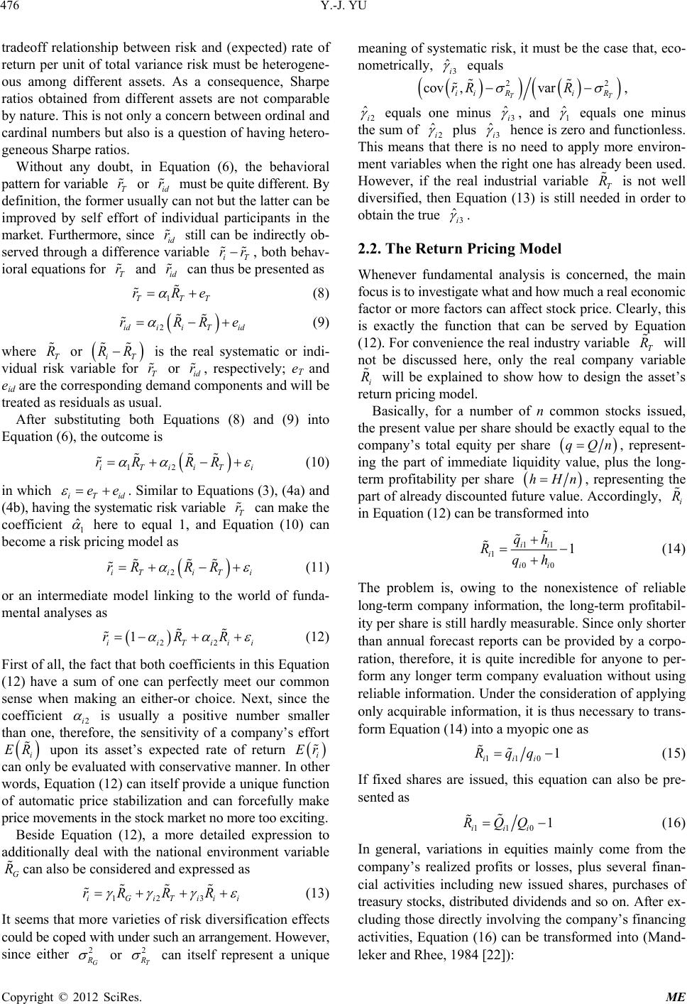

Y.-J. YU

476

tradeoff relationship between risk and (expected) rate of

return per unit of total variance risk must be heterogene-

ous among different assets. As a consequence, Sharpe

ratios obtained from different assets are not comparable

by nature. This is not only a concern between ordinal and

cardinal numbers but also is a question of having hetero-

geneous Sharpe ratios.

Without any doubt, in Equation (6), the behavioral

pattern for variable T or id

r must be quite different. By

definition, the former usually can not but the latter can be

improved by self effort of individual participants in the

market. Furthermore, since id still can be indirectly ob-

served through a difference variable iT

, both behav-

ioral equations for and can thus be presented as

 









1TTT

rRe









i Tid

rRRe





RR



r



 (8)

2id i



 (9)

where T or iT

is the real systematic or indi-

vidual risk variable for T or id, respectively; eT and

eid are the corresponding demand components and will be

treated as residuals as usual.



After substituting both Equations (8) and (9) into

Equation (6), the outcome is





iiT

12iT

rR i











 (10)

in which iTid







. Similar to Equations (3), (4a) and

(4b), having the systematic risk variable T can make the

coefficient 1



here to equal 1, and Equation (10) can

become a risk pricing model as





iT i

2iTi





 



22Tii



 (11)

or an intermediate model linking to the world of funda-

mental analyses as



rR i





 





 (12)

First of all, the fact that both coefficients in this Equation

(12) have a sum of one can perfectly meet our common

sense when making an either-or choice. Next, since the

coefficient 2i



is usually a positive number smaller

than one, therefore, the sensitivity of a company’s effort

i upon its asset’s expected rate of return











3iTii

R R

can only be evaluated with conservative manner. In other

words, Equation (12) can itself provide a unique function

of automatic price stabilization and can forcefully make

price movements in the stock market no more too exciting.

Beside Equation (12), a more detailed expression to

additionally deal with the national environment variable

can also be considered and expressed as

12iG

rR i

 











 (13)

It seems that more varieties of risk diversification effects

could be coped with under such an arrangement. However,

since either



or 2



can itself represent a unique

meaning of systematic risk, it must be the case that, eco-

nometrically, 3

ˆi



equals











cov ,var

ii Ri R

rR R











equals one minus 3

ˆi



, and 1



equals one minus

the sum of 2i



plus 3i



hence is zero and functionless.

This means that there is no need to apply more environ-

ment variables when the right one has already been used.

However, if the real industrial variable T is not well

diversified, then Equation (13) is still needed in order to

obtain the true



ˆi



2.2. The Return Pricing Model

Whenever fundamental analysis is concerned, the main

focus is to investigate what and how much a real economic

factor or more factors can affect stock price. Clearly, this

is exactly the function that can be served by Equation

(12). For convenience the real industry variable T will

not be discussed here, only the real company varia

 will be explained to show how to design the asset’s

return pricing model.



ble

Basically, for a number of n common stocks issued,

the present value per share should be exactly equal to the

company’s total equity per share



qQn, represent-

ing the part of immediate liquidity value, plus the long-

term profitability per share



hHn



, representing the

part of already discounted future value. Accordingly,

in Equation (12) can be transformed into

Rqh











 (14)

The problem is, owing to the nonexistence of reliable

long-term company information, the long-term profitabil-

ity per share is still hardly measurable. Since only shorter

than annual forecast reports can be provided by a corpo-

ration, therefore, it is quite incredible for anyone to per-

form any longer term company evaluation without using

reliable information. Under the consideration of applying

only acquirable information, it is thus necessary to trans-

form Equation (14) into a myopic one as

110

iii

Rqq





 (15)

If fixed shares are issued, this equation can also be pre-

sented as

110

iii

RQQ







 (16)

In general, variations in equities mainly come from the

company’s realized profits or losses, plus several finan-

cial activities including new issued shares, purchases of

treasury stocks, distributed dividends and so on. After ex-

cluding those directly involving the company’s financing

activities, Equation (16) can be transformed into (Mand-

leker and Rhee, 1984 [22]):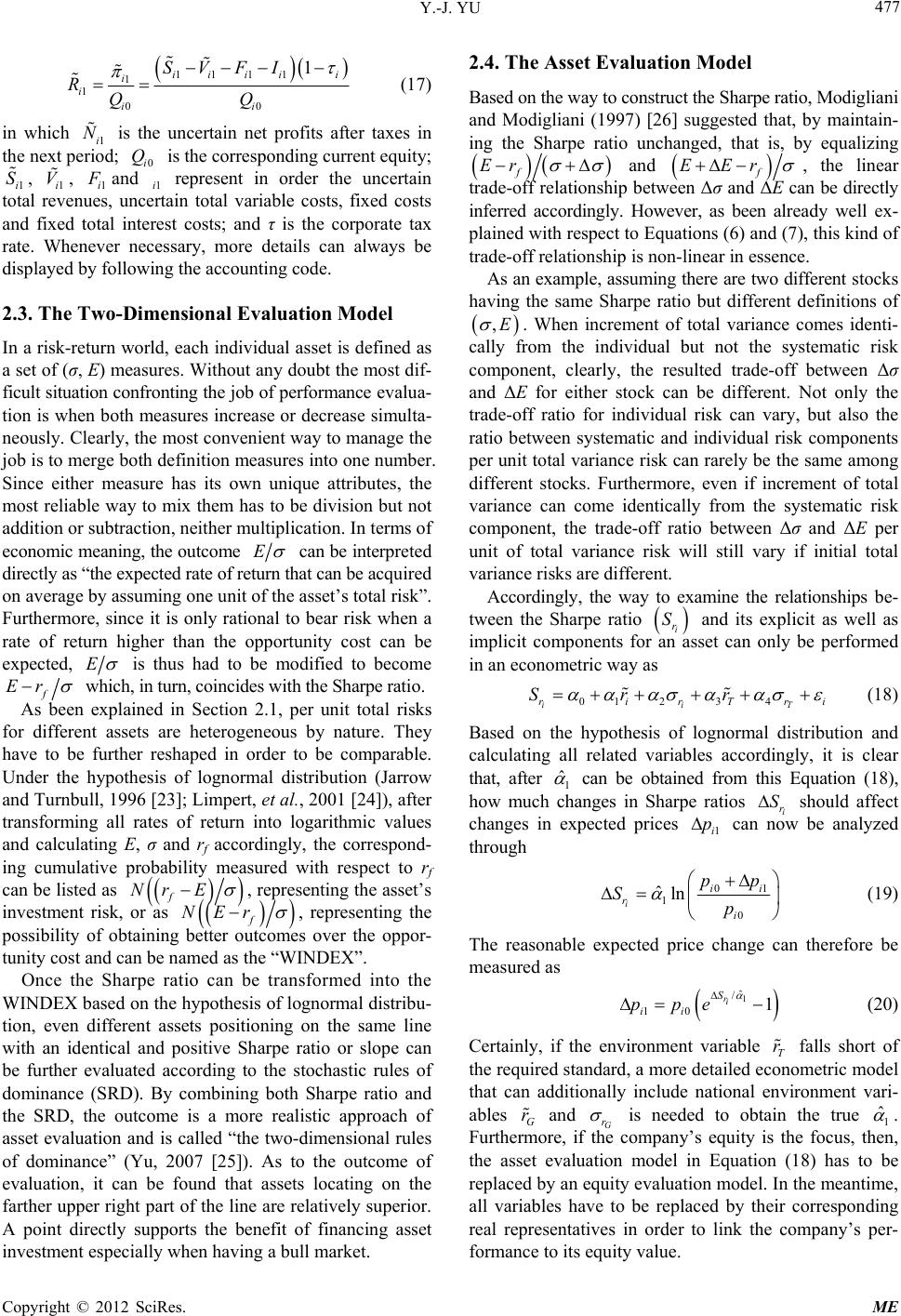

Y.-J. YU 477



SV F

RQQ

iii













 



(17)

in which 1i is the uncertain net profits after taxes in

the next period; i is the corresponding current equity;

1i, 1i, 1i



and 1i represent in order the uncertain

total revenues, uncertain total variable costs, fixed costs

and fixed total interest costs; and τ is the corporate tax

rate. Whenever necessary, more details can always be

displayed by following the accounting code.

2.3. The Two-Dimensional Evaluation Model

In a risk-return world, each individual asset is defined as

a set of (σ, E) measures. Without any doubt the most dif-

ficult situation confronting the job of performance evalua-

tion is when both measures increase or decrease simulta-

neously. Clearly, the most convenient way to manage the

job is to merge both definition measures into one number.

Since either measure has its own unique attributes, the

most reliable way to mix them has to be division but not

addition or subtraction, neither multiplication. In terms of

economic meaning, the outcome E



can be interpreted

directly as “the expected rate of return that can be acquired

on average by assuming one unit of the asset’s total risk”.

Furthermore, since it is only rational to bear risk when a

rate of return higher than the opportunity cost can be

expected, E



is thus had to be modified to become







which, in turn, coincides with the Sharpe ratio.

As been explained in Section 2.1, per unit total risks

for different assets are heterogeneous by nature. They

have to be further reshaped in order to be comparable.

Under the hypothesis of lognormal distribution (Jarrow

and Turnbull, 1996 [23]; Limpert, et al., 2001 [24]), after

transforming all rates of return into logarithmic values

and calculating E, σ and rf accordingly, the correspond-

ing cumulative probability measured with respect to rf

can be listed as



Nr E







, representing the asset’s

investment risk, or as



NEr



, representing the

possibility of obtaining better outcomes over the oppor-

tunity cost and can be named as the “WINDEX”.

Once the Sharpe ratio can be transformed into the

WINDEX based on the hypothesis of lognormal distribu-

tion, even different assets positioning on the same line

with an identical and positive Sharpe ratio or slope can

be further evaluated according to the stochastic rules of

dominance (SRD). By combining both Sharpe ratio and

the SRD, the outcome is a more realistic approach of

asset evaluation and is called “the two-dimensional rules

of dominance” (Yu, 2007 [25]). As to the outcome of

evaluation, it can be found that assets locating on the

farther upper right part of the line are relatively superior.

A point directly supports the benefit of financing asset

investment especially when having a bull market.

2.4. The Asset Evaluation Model

Based on the way to construct the Sharpe ratio, Modigliani

and Modigliani (1997) [26] suggested that, by maintain-

ing the Sharpe ratio unchanged, that is, by equalizing













Er EEr



 and





 , the linear

trade-off relationship between Δσ and ΔE can be directly

inferred accordingly. However, as been already well ex-

plained with respect to Equations (6) and (7), this kind of

trade-off relationship is non-linear in essence.

As an example, assuming there are two different stocks

having the same Sharpe ratio but different definitions of







. When increment of total variance comes identi-

cally from the individual but not the systematic risk

component, clearly, the resulted trade-off between Δσ

and ΔE for either stock can be different. Not only the

trade-off ratio for individual risk can vary, but also the

ratio between systematic and individual risk components

per unit total variance risk can rarely be the same among

different stocks. Furthermore, even if increment of total

variance can come identically from the systematic risk

component, the trade-off ratio between Δσ and ΔE per

unit of total variance risk will still vary if initial total

variance risks are different.

Accordingly, the way to examine the relationships be-

tween the Sharpe ratio





01 234

iiT

rirTri

Sr r

r and its explicit as well as

implicit components for an asset can only be performed

in an econometric way as



 



 



(18)

Based on the hypothesis of lognormal distribution and

calculating all related variables accordingly, it is clear

that, after 1



can be obtained from this Equation (18),

how much changes in Sharpe ratios i

r should affect

changes in expected prices can now be analyzed

through

S

p

ˆln







 





10 1

ppe





(19)

The reasonable expected price change can therefore be

measured as







(20)

Certainly, if the environment variable T falls short of

the required standard, a more detailed econometric model

that can additionally include national environment vari-

ables G and G



is needed to obtain the true 1



Furthermore, if the company’s equity is the focus, then,

the asset evaluation model in Equation (18) has to be

replaced by an equity evaluation model. In the meantime,

all variables have to be replaced by their corresponding

real representatives in order to link the company’s per-

formance to its equity value.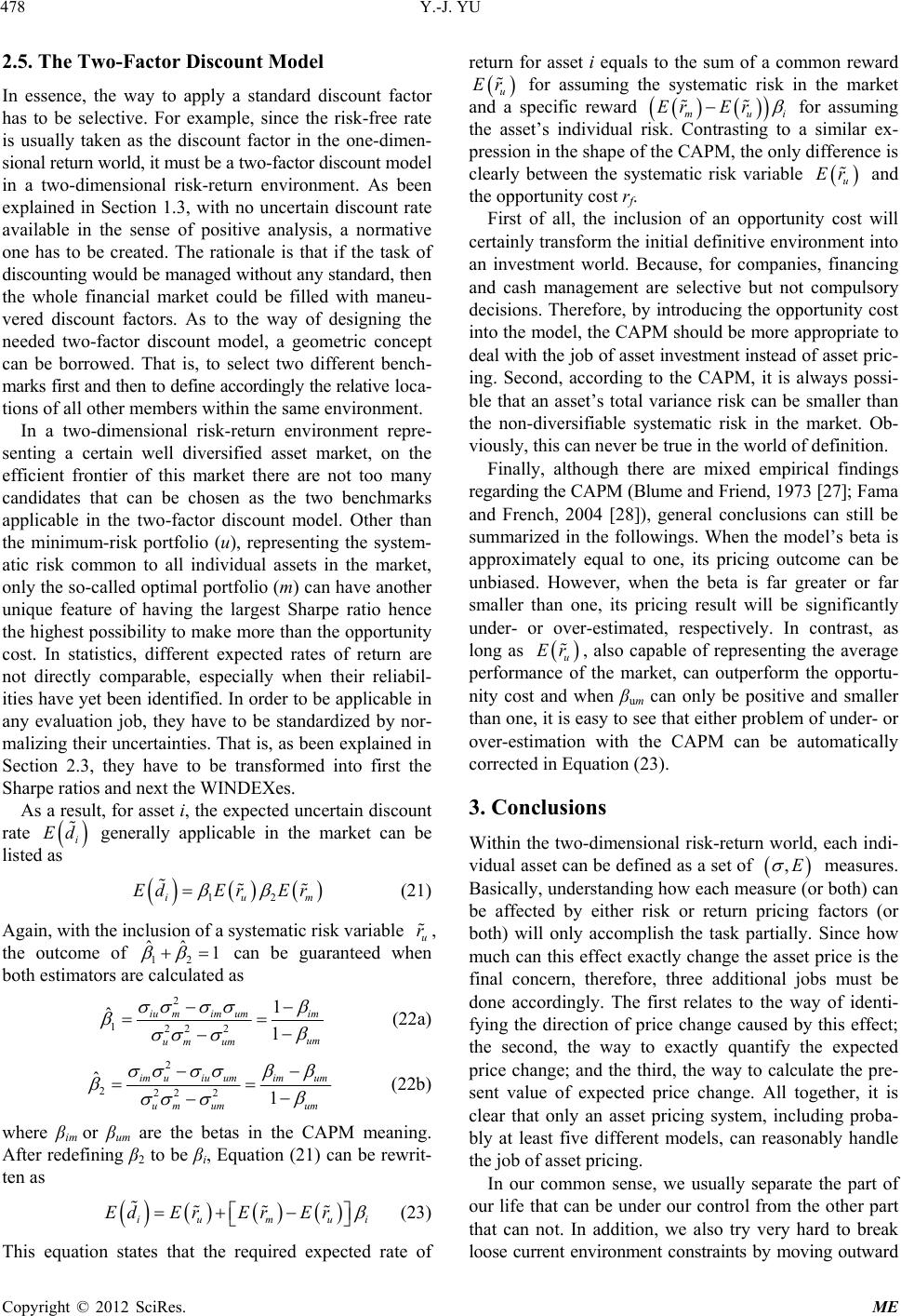

Y.-J. YU

478

2.5. The Two-Factor Discount Model

In essence, the way to apply a standard discount factor

has to be selective. For example, since the risk-free rate

is usually taken as the discount factor in the one-dimen-

sional return world, it must be a two-factor discount model

in a two-dimensional risk-return environment. As been

explained in Section 1.3, with no uncertain discount rate

available in the sense of positive analysis, a normative

one has to be created. The rationale is that if the task of

discounting would be managed without any standard, then

the whole financial market could be filled with maneu-

vered discount factors. As to the way of designing the

needed two-factor discount model, a geometric concept

can be borrowed. That is, to select two different bench-

marks first and then to define accordingly the relative loca-

tions of all other members within the same environment.

In a two-dimensional risk-return environment repre-

senting a certain well diversified asset market, on the

efficient frontier of this market there are not too many

candidates that can be chosen as the two benchmarks

applicable in the two-factor discount model. Other than

the minimum-risk portfolio (u), representing the system-

atic risk common to all individual assets in the market,

only the so-called optimal portfolio (m) can have another

unique feature of having the largest Sharpe ratio hence

the highest possibility to make more than the opportunity

cost. In statistics, different expected rates of return are

not directly comparable, especially when their reliabil-

ities have yet been identified. In order to be applicable in

any evaluation job, they have to be standardized by nor-

malizing their uncertainties. That is, as been explained in

Section 2.3, they have to be transformed into first the

Sharpe ratios and next the WINDEXes.

As a result, for asset i, the expected uncertain discount

rate generally applicable in the market can be

listed as





 

12ium

Er Er





th ˆ







Ed 

 (21)

Again, with the inclusion of a systematic risk variable u

,

e outcome of 12



can be guaranteed when

both estimators are calculated as

122

ˆiu mim

um im







 









 (22a)

222 2

ˆim uiu um

um um1

im um





 





 









 

mui

(22b)

where βim or βum are the betas in the CAPM meaning.

After redefining β2 to be βi, Equation (21) can be rewrit-

ten as



 

Ed ErEr















 (23)

This equation states that the required expected rate of

return for asset i equals to the sum of a common reward







u for assuming the systematic risk in the market

and a specific reward







mui

Er Er







for assuming

the asset’s individual risk. Contrasting to a similar ex-

pression in the shape of the CAPM, the only difference is

clearly between the systematic risk variable





 and

the opportunity cost rf.

First of all, the inclusion of an opportunity cost will

certainly transform the initial definitive environment into

an investment world. Because, for companies, financing

and cash management are selective but not compulsory

decisions. Therefore, by introducing the opportunity cost

into the model, the CAPM should be more appropriate to

deal with the job of asset investment instead of asset pric-

ing. Second, according to the CAPM, it is always possi-

ble that an asset’s total variance risk can be smaller than

the non-diversifiable systematic risk in the market. Ob-

viously, this can never be true in the world of definition.

Finally, although there are mixed empirical findings

regarding the CAPM (Blume and Friend, 1973 [27]; Fama

and French, 2004 [28]), general conclusions can still be

summarized in the followings. When the model’s beta is

approximately equal to one, its pricing outcome can be

unbiased. However, when the beta is far greater or far

smaller than one, its pricing result will be significantly

under- or over-estimated, respectively. In contrast, as

long as











u, also capable of representing the average

performance of the market, can outperform the opportu-

nity cost and when βum can only be positive and smaller

than one, it is easy to see that either problem of under- or

over-estimation with the CAPM can be automatically

corrected in Equation (23).

3. Conclusions

Within the two-dimensional risk-return world, each indi-

vidual asset can be defined as a set of measures.

Basically, understanding how each measure (or both) can

be affected by either risk or return pricing factors (or

both) will only accomplish the task partially. Since how

much can this effect exactly change the asset price is the

final concern, therefore, three additional jobs must be

done accordingly. The first relates to the way of identi-

fying the direction of price change caused by this effect;

the second, the way to exactly quantify the expected

price change; and the third, the way to calculate the pre-

sent value of expected price change. All together, it is

clear that only an asset pricing system, including proba-

bly at least five different models, can reasonably handle

the job of asset pricing.

In our common sense, we usually separate the part of

our life that can be under our control from the other part

that can not. In addition, we also try very hard to break

loose current environment constraints by moving outward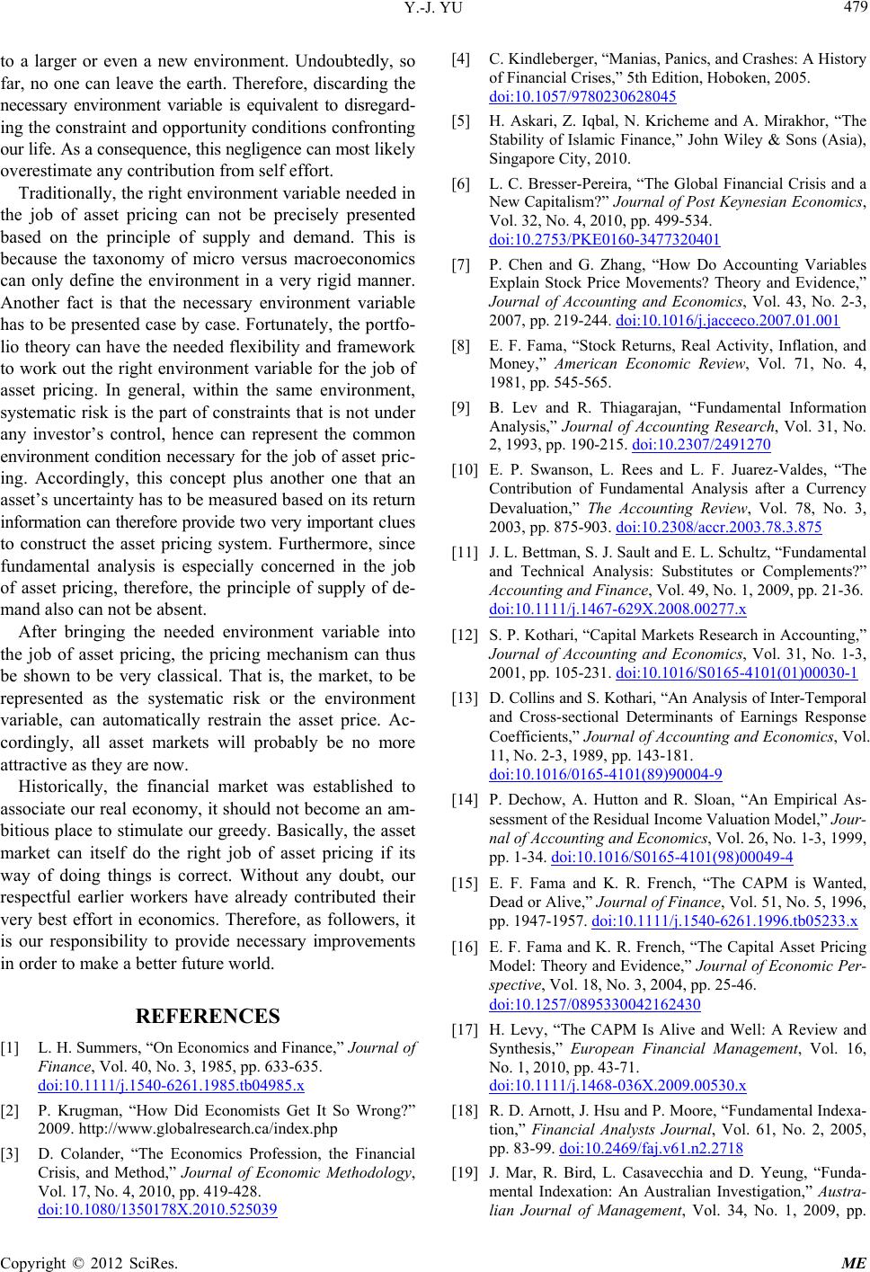

Y.-J. YU 479

to a larger or even a new environment. Undoubtedly, so

far, no one can leave the earth. Therefore, discarding the

necessary environment variable is equivalent to disregard-

ing the constraint and opportunity conditions confronting

our life. As a consequence, this negligence can most likely

overestimate any contribution from self effort.

Traditionally, the right environment variable needed in

the job of asset pricing can not be precisely presented

based on the principle of supply and demand. This is

because the taxonomy of micro versus macroeconomics

can only define the environment in a very rigid manner.

Another fact is that the necessary environment variable

has to be presented case by case. Fortunately, the portfo-

lio theory can have the needed flexibility and framework

to work out the right environment variable for the job of

asset pricing. In general, within the same environment,

systematic risk is the part of constraints that is not under

any investor’s control, hence can represent the common

environment condition necessary for the job of asset pric-

ing. Accordingly, this concept plus another one that an

asset’s uncertainty has to be measured based on its return

information can therefore provide two very important clues

to construct the asset pricing system. Furthermore, since

fundamental analysis is especially concerned in the job

of asset pricing, therefore, the principle of supply of de-

mand also can not be absent.

After bringing the needed environment variable into

the job of asset pricing, the pricing mechanism can thus

be shown to be very classical. That is, the market, to be

represented as the systematic risk or the environment

variable, can automatically restrain the asset price. Ac-

cordingly, all asset markets will probably be no more

attractive as they are now.

Historically, the financial market was established to

associate our real economy, it should not become an am-

bitious place to stimulate our greedy. Basically, the asset

market can itself do the right job of asset pricing if its

way of doing things is correct. Without any doubt, our

respectful earlier workers have already contributed their

very best effort in economics. Therefore, as followers, it

is our responsibility to provide necessary improvements

in order to make a better future world.

REFERENCES

[1] L. H. Summers, “On Economics and Finance,” Journal of

Finance, Vol. 40, No. 3, 1985, pp. 633-635.

doi:10.1111/j.1540-6261.1985.tb04985.x

[2] P. Krugman, “How Did Economists Get It So Wrong?”

2009. http://www.globalresearch.ca/index.php

[3] D. Colander, “The Economics Profession, the Financial

Crisis, and Method,” Journal of Economic Methodology,

Vol. 17, No. 4, 2010, pp. 419-428.

doi:10.1080/1350178X.2010.525039

[4] C. Kindleberger, “Manias, Panics, and Crashes: A History

of Financial Crises,” 5th Edition, Hoboken, 2005.

doi:10.1057/9780230628045

[5] H. Askari, Z. Iqbal, N. Kricheme and A. Mirakhor, “The

Stability of Islamic Finance,” John Wiley & Sons (Asia),

Singapore City, 2010.

[6] L. C. Bresser-Pereira, “The Global Financial Crisis and a

New Capitalism?” Journal of Post Keynesian Economics,

Vol. 32, No. 4, 2010, pp. 499-534.

doi:10.2753/PKE0160-3477320401

[7] P. Chen and G. Zhang, “How Do Accounting Variables

Explain Stock Price Movements? Theory and Evidence,”

Journal of Accounting and Economics, Vol. 43, No. 2-3,

2007, pp. 219-244. doi:10.1016/j.jacceco.2007.01.001

[8] E. F. Fama, “Stock Returns, Real Activity, Inflation, and

Money,” American Economic Review, Vol. 71, No. 4,

1981, pp. 545-565.

[9] B. Lev and R. Thiagarajan, “Fundamental Information

Analysis,” Journal of Accounting Research, Vol. 31, No.

2, 1993, pp. 190-215. doi:10.2307/2491270

[10] E. P. Swanson, L. Rees and L. F. Juarez-Valdes, “The

Contribution of Fundamental Analysis after a Currency

Devaluation,” The Accounting Review, Vol. 78, No. 3,

2003, pp. 875-903. doi:10.2308/accr.2003.78.3.875

[11] J. L. Bettman, S. J. Sault and E. L. Schultz, “Fundamental

and Technical Analysis: Substitutes or Complements?”

Accounting and Finance, Vol. 49, No. 1, 2009, pp. 21-36.

doi:10.1111/j.1467-629X.2008.00277.x

[12] S. P. Kothari, “Capital Markets Research in Accounting,”

Journal of Accounting and Economics, Vol. 31, No. 1-3,

2001, pp. 105-231. doi:10.1016/S0165-4101(01)00030-1

[13] D. Collins and S. Kothari, “An Analysis of Inter-Temporal

and Cross-sectional Determinants of Earnings Response

Coefficients,” Journal of Accounting and Economics, Vol.

11, No. 2-3, 1989, pp. 143-181.

doi:10.1016/0165-4101(89)90004-9

[14] P. Dechow, A. Hutton and R. Sloan, “An Empirical As-

sessment of the Residual Income Valuation Model,” Jour-

nal of Accounting and Economics, Vol. 26, No. 1-3, 1999,

pp. 1-34. doi:10.1016/S0165-4101(98)00049-4

[15] E. F. Fama and K. R. French, “The CAPM is Wanted,

Dead or Alive,” Journal of Finance, Vol. 51, No. 5, 1996,

pp. 1947-1957. doi:10.1111/j.1540-6261.1996.tb05233.x

[16] E. F. Fama and K. R. French, “The Capital Asset Pricing

Model: Theory and Evidence,” Journal of Economic Per-

spective, Vol. 18, No. 3, 2004, pp. 25-46.

doi:10.1257/0895330042162430

[17] H. Levy, “The CAPM Is Alive and Well: A Review and

Synthesis,” European Financial Management, Vol. 16,

No. 1, 2010, pp. 43-71.

doi:10.1111/j.1468-036X.2009.00530.x

[18] R. D. Arnott, J. Hsu and P. Moore, “Fundamental Indexa-

tion,” Financial Analysts Journal, Vol. 61, No. 2, 2005,

pp. 83-99. doi:10.2469/faj.v61.n2.2718

[19] J. Mar, R. Bird, L. Casavecchia and D. Yeung, “Funda-

mental Indexation: An Australian Investigation,” Austra-

lian Journal of Management, Vol. 34, No. 1, 2009, pp.

Y.-J. YU

480

1-20. doi:10.1177/031289620903400102

[20] P. D. Kaplan, “Why Fundamental Indexation Might—Or

Might Not—WORK,” Financial Analysts Journal, Vol.

64, No. 1, 2008, pp. 32-39. doi:10.2469/faj.v64.n1.5

[21] F. J. Fabozzi, F. Gupta and H. M. Markowitz, “The Leg-

acy of Modern Portfolio Theory,” Journal of Investing,

Vol. 11, No. 3, 2002, pp. 7-22.

doi:10.3905/joi.2002.319510

[22] G. N. Mandelker and S. G. Rhee, “The Impact of the

Degree of Operating and Financial Leverage on System-

atic Risk of Common Stock,” Journal of Financial and

Quantitative Analysis, Vol. 19, No. 1, 1984, pp. 45-57.

doi:10.2307/2331000

[23] R. Jarrow and S. Turnbull, “Derivative Securities,” Chap-

ter 4, South-Western, Cincinnati, 1996.

[24] E. Limpert, W. A. Stahel and M. Abbt, “Log-normal Dis-

tribution across the Sciences: Keys and Clues,” Biosci-

ence, Vol. 51, No. 5, 2001, pp. 341-352.

doi:10.1641/0006-3568(2001)051[0341:LNDATS]2.0.C

O;2

[25] Y. Yu, “Stock Analysis and Investment,” 2nd Edition, (in

Chinese), Yeh-Yeh, Taipei, 2007.

[26] F. Modigliani and L. Modigliani, “Risk-Adjusted Per-

formance,” Journal of Portfolio Management, Vol. 23,

No. 2, 1997, pp. 45-54. doi:10.3905/jpm.23.2.45

[27] M. Blume and I. Friend, “A New Look at the Capital

Asset Pricing Model,” Journal of Finance, Vol. 28, No. 1,

1973, pp. 19-34. doi:10.1111/j.1540-6261.1973.tb01342.x

[28] E. F. Fama and K. R. French, “The Capital Asset Pricing

Model: Theory and Evidence,” Journal of Economic

Perspective, Vol. 18, No. 3, 2004, pp. 25-46.

doi:10.1257/0895330042162430