World Journal of Nano Science and Engineering, 2012, 2, 154-160
http://dx.doi.org/10.4236/wjnse.2012.23020 Published Online September 2012 (http://www.SciRP.org/journal/wjnse)
Modified Scherrer Equation to Estimate More Accurately
Nano-Crystallite Size Using XRD
Ahmad Monshi*, Mohammad Reza Foroughi#, Mohammad Reza Monshi
Department of Materials Engineering, Najafabad branch, Islamic Azad University, Isfahan, Iran
Email: *a-monshi@cc.iut.ac.ir, #foroughi@iaun.ac.ir
Received July 20, 2012; revised August 20, 2012; accepted August 28, 2012
ABSTRACT
Scherrer Equation, .cosLK
, was developed in 1918, to calculate the nano crystallite size (L) by XRD radiation
of wavelength λ (nm) from measuring full width at half maximum of peaks (β) in radian located at any 2θ in the pattern.
Shape factor of K can be 0.62 - 2.08 and is usually taken as about 0.89. But, if all of the peaks of a pattern are going to
give a similar value of L, then .cosθ
must be identical. This means that for a typical 5nm crystallite size and λ Cukα1
= 0.15405 nm the peak at 2θ = 170˚ must be more than ten times wide with respect to the peak at 2θ = 10˚, which is
never observed. The purpose of modified Scherrer equation given in this paper is to provide a new approach to the kind
of using Scherrer equation, so that a least squares technique can be applied to minimize the sources of errors. Modified
Scherrer equation plots lnβ against ln(1/cosθ) and obtains the intercept of a least squares line regression, ln /
K
L
,
from which a single value of L is obtained through all of the available peaks. This novel technique is used for a natural
Hydroxyapatite (HA) of bovine bone fired at 600˚C, 700˚C, 900˚C and 1100˚C from which nano crystallite sizes of 22.8,
35.5, 37.3 and 38.1 nm were respectively obtained and 900˚C was selected for biomaterials purposes. These results
show that modified Scherrer equation method is promising in nano materials applications and can distinguish between
37.3 and 38.1 nm by using the data from all of the available peaks.
Keywords: X-Ray Diffraction; Nano-Crystal; Scherrer Equation; Hydroxyapatite
1. Introduction
X-ray diffraction is a convenient method for determining
the mean size of nano crystallites in nano crystalline bulk
materials. The first scientist, Paul Scherrer, published his
results in a paper that included what became known as
the Scherrer equation in 1981 [1].
This can be attributed to the fact that “crystallite size”
is not synonymous with “particle size”, while X-Ray
diffraction is sensitive to the crystallite size inside the
particles. From the well-known Scherrer formula the
average crystallite size, L, is:
.cos
K
L
(1)
where λ is the X-ray wavelength in nanometer (nm), β is
the peak width of the diffraction peak profile at half
maximum height resulting from small crystallite size in
radians and K is a constant related to crystallite shape,
normally taken as 0.9. The value of β in 2θ axis of
diffraction profile must be in radians. The θ can be in
degrees or radians, since the cosθ corresponds to the
same number;
π2
coscos 45
42
 (2)
It can be taken as 0.89 or 0.9 for Full Width Half
Maximum (FWHM) of spherical crystals with cubic unit
cells. For an excellent discussion of K, a good reference
is the paper “Scherrer after sixty years” in 1978 [2].
In conventional approximation, the integrated width of
the pure profile (β) is separated from that of the observed
diffraction profile (B) assuming that both profiles are
either Gaussian or Cauchy [3].
If Gaussian profile is accepted, then 22
Bb 2
 in
the case of Cauchy B = b + β, where b is the instrument
profile width. If the broadening of the pure profile is due
to both crystallite size and lattice strain, one has to make
another assumption concerning the shapes of the two
contributing line profiles. Normally, these are supposed
to be either Gaussian or both Cauchy, then 22
mn


or, mn

respectively. m
is the line width re-
sulting from small crystallite size, and n
is the line
broadening due to the lattice strain. Then we have [4]:
4.tg
n
(3)
*#Corresponding authors.
C
opyright © 2012 SciRes. WJNSE
A. MONSHI ET AL. 155
Strain = Change in size/Original size (4)
It is usually considered that Cauchy function is rather
well approximated, while Gaussian function gave
considerably larger errors. In order to separate the size
and strain contribution:
4.tg
.cosL

 (5)
In the case of crystallite size and lattice strain, two
diffraction peaks must be used to calculate two unknown
parameters L and ε.
In order to consider the Scherrer equation with
obtained value of ε concerning only crystallite size, when
no mechanical activation such as ball milling and
mechanical alloying is the case, or the crystallite size is
due to a nucleation and growth at high temperatures, we
must only be concerned about corrections for instru-
mental profile width.
The Scherrer equation predicts crystallite thickness if
crystals are smaller than 1000 Å or 100 nm. The simplest
way to obtain Scherrer equation is to take the derivation
of Bragg’s Law, 2sind
.
Holding the wavelength λ constant and allowing the
diffraction angle to broaden from a sharp diffraction peak
from an infinite single crystal with perfect 3-dimeintinal
order. For a single crystal, the diffraction from a set of
planes with the distance d* occurs at a precisely θ*, so
that λ = 2d*sinθ*.
For many small nano crystals, diffraction from a lot of
tiny crystals deviate ± Δθ from θ*.
This means 2Δθ on the 2θ axis of diffraction pattern.
The value of Δθ correspond to FWHM or β, which is
approximately half of 2Δθ. In other words since Δθ can
be positive or negative, the absolute value must be taken
and it reflects the half width of the shape line deviation in
2θ axis (full width at half maximum height, β). Deriva-
tive in d and θ of Bragg’s Law with constant λ gives λ =
2Δd.cosθ.Δθ.
The thickness Δd = L can be taken as;
2cos .Δcos.
Ld


 
(6)
By applying a shape factor K, which is near the value
of unit (0.9), the Scherrer equation can be given as:
0.9
.cos
L
(7)
The derivation approach is taken by Alexander in Klug
and Alexander “X-ray Diffraction” [3] to describe the
Scherrer equation. It is also easily adoptable to describe
the dependence of any two terms in the Bragg equation
in terms of variability. For crystals longer than 1000 Å
(100 nm), grainy patterns can be analyzed in terms of a
statistical analysis to grain size, although this is rarely
done since grain size can be more easily determined from
optical or electron microscopy studies in this size range.
2. Modified Scherrer Equation
It is assumed that if there are N different peaks of a
specific nano crystal in the range of 0 - 180˚ (2θ) or 0 -
90˚ (θ), then all of these N peaks must present identical L
values for the crystal size. But, during the extensive
research of the first author of thins paper, on different
nano ceramic crystals, which were synthesized or mi-
nerally achieved, it was surprisingly observed that each
peak yields a different value and there is a systematic
error on the results obtained from each peak.
Further investigation approved the presence of a sys-
tematic error in Scherrer formula. In fact since
.cosLK

, if L is going to be a fixed value for
different peaks of a substance, considering that K and λ
and therefore Kλ are fixed values, then it is essential that
β.cosθ be a fixed multiple during 0 < 2θ < 180˚ or 0 < θ
< 90˚. Suppose that for a crystallite size of 5nm, obtained
at a peak of say 2θ = 10˚ (θ = 5˚) by using K = 0.89 and
λCukα1 = 0.15405 nm.
then β10 must be,

10
0.89 0.154050.0275 1.576
5cos5 rad

(8)
Now, suppose that the N th peak of this nano crystal
occurs at 2θ = 170˚ (or θ = 85˚), then;

170
0.89 0.154050.3146 18.03
5cos85 rad

(9)
This means that the ratio of 18.03 1.57611.44
must be applied170 10
/
for


. In other words if the first
peak has a β10 of around 2 mm on the monitor of
computer plot, or for example, a paper plot 21 cm width
on A4 paper, then the last peak must have a β170 more
than 22.88 mm and a base of peak more than 45.76 mm
(4.576 cm).
This has never been observed and cannot be true.
Modified Scherrer formula is based on the face that we
must decrease the errors and obtain the average value of
L though all the peaks (or any number of selected peaks)
by using least squares method to mathematically de-
crease the source of errors.
We can write the basic Scherrer formula as:
1
.
.cos cos
KK
LL

 (10)
Now by making logarithm on both sides;
1
ln lnlnln
.cos cos
KK
LL

 (11)
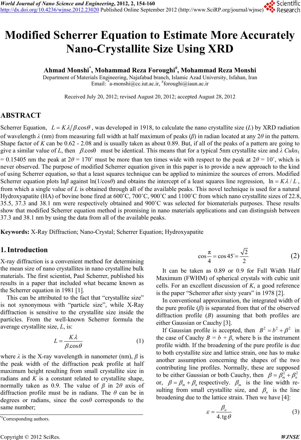
If we plot the results of lnβ against ln(1cos
), then a
straight line with a slope of around one and an intercept
Copyright © 2012 SciRes. WJNSE
A. MONSHI ET AL.
Copyright © 2012 SciRes. WJNSE
156
3. Experimental
of about lnK/L must be obtained. Theoretically this
straight line must be with a slope of 45˚ since tg45˚ = 1
(Figure 1). But, since errors are associated with ex-
perimental data, the least squares method gives the best
slope and most accurate lnK/L. After getting the inter-
cept, then the exponential of the intercept is obtained:
Bovine bones were boiled for 2 hr to remove flesh and
fat. The bones were heated at 60˚C for 24 hr to remove
moisture. To prevent blackening with soot during heating,
the bones are cut into small pieces of about 10 mm thick
and heated at 400˚C (bone ash) for 3 hr in air to allow for
evaporation of organic substances. The resulting black
bone ash was heated for 2 hr at 600˚C, 700˚C, 900˚C and
1100˚C [5].
ln K
L
K
eL
(12)
Having K = 0.9 and λ(such as λCukα1 = 0.15405 nm), a
single value of L in nanometer can be calculated. A Philips XRD instrument with Cukα radiation using
40 KV and 30 mA, step size of 0.05˚ (2θ) and scan rate of
1˚/min were employed. X’Pert software was used for
qualitative analysis and report of β values at FWHM at
different 2θ values according to location of the peaks.
According to JCPDS:9-432 standard the main peaks are
from the planes of (200), (111), (002), (102), (210), (211),
(112), (300), (202), (212), (310), (311), (113), (222),
(312) and (213) of HA phase for 20 - 50 deg. 2θ.
In (1/cosθ)
In β
4. Results and Discussion
Table 1 shows the β.cosθ values for different peaks at
any given temperature.
The XRD patterns are observed in Figure 2 with
gradual sharpness of the peaks as the soaking temper-
ature increases, indicating the growth and increase of
crystallite size.
Relatively gradual decrease in β.cosθ and almost
increase in L values (./.cosLconst )
is observed
with the increase of 2θ. Such as increase in crystallite
Figure 1. Modified scherrer equation plot.
Table 1. Values of β.cosθ for different peaks.
Temperature (˚C)
d
400 600 700 900 1100
Calculated L at 900˚C (nm)
(200) – – 5.06 × 10³ 5.06 × 10³ 5.06 × 10³ 27.1
(111) 5.05 × 10³ 5.05 × 10³ 27.1
(002) 2.24 × 10³ 5.02 × 10³ 3.35 × 10³ 3.35 × 10³ 3.35 × 10³ 40.9
(102) – 2.50 × 10³ 3.34 × 10³ 2.50 × 10³ 41
(210) – – 3.23 × 10³ 2.50 × 10³ 42.4
(211) 9.90 × 10³ 11.5 × 10³ 2.48 × 10³ 3.31 × 10³ 2.48 × 10³ 41.4
(112) – – 2.48 × 10³ 2.48 × 10³ 2.48 × 10³ 55.2
(300) – – 2.47 × 10³ 3.30 × 10³ 3.30 × 10³ 41.5
(202) – – 3.29 × 10³ 3.29 × 10³ 3.29 × 10³ 41.6
(212) – – – 2.43 × 10³ 2.43 × 10³ 56.4
(310) 11.3 × 10³ 12.9 × 10³ 2.42 × 10³ 2.16 × 10³ 3.23 × 10³ 63.4
(311) – – 2.41 × 10³ 4.81 × 10³ 2.41 × 10³ 28.5
(113) – – 3.19 × 10³ 6.38 × 10³ 3.19 × 10³ 21.5
(222) 7.88 × 10³ 7.88 × 10³ 3.16 × 10³ 2.11 × 10³ 3.16 × 10³ 65
(312) – – 3.14 × 10³ 3.14 × 10³ 3.14 × 10³ 43.6
(213) 9.35 × 10³ 6.25 × 10³ 3.89 × 10³ 3.12 × 10³ 2.09 × 10³ 44
A. MONSHI ET AL. 157
Figure 2. Patterns of XRD analysis related to natural HA of thermal analysis at temperatures of: (a) 400˚C (bone ash); (b)
600˚C; (c) 700˚C; (d) 900˚C and (e) 1100˚C.
size of HA were also observed by Shipmen et al. [6]. The
samples fired at 600˚C - 1100˚C were used.
Figure 3 indicates four plots of lnβ vs. ln(1cos
) for
individual soaking temperatures; together with the equa-
tions of linear least squares method obtained from linear
regression of data in excel plots. Due to sources of error
in measuring β and treating for different available peaks,
since the β.cosθ multiple is not really a constant value for
all the peaks, π
 
deviate from 45˚ and are negative
in some cases. The reason that the slopes are negative are
due to the fact that at higher angles, of 2θ, with lower
values of cosθ and higher values of ln(1cos
), the
amounts of β observed and measured are less than it must
be according to Scherrer’s formula. This means that a 45˚
slope for the linear plots are hardly achieved. The errors
involved in Scherrer equation when employing different
peaks are the main cause of scattering of the points.
Some other sources of error are measuring ln
and
ln(1cos
). The significance of this work is to minimize
the errors by applying a method to use least squares
technique for obtaining the best results.
The modified Scherrer equation can provide the
advantage of decreasing the sum of absolute values of
errors,
2
ln

49 5.1196yx
4.8149ln1/ cos
, and producing a single line through
the points to give a single value of intercept lnK/L. At
600˚C, the linear regression plot is obtained as
. This is equivalent to
4.81
ln

ln /
K
L
KL
e
.006
. From this line, the
intercept is 5.1196 and and
5.1196
/0
0.890.15405/ 0.00622.8nmL
(13)
It is interesting to notice that although variations exist
in lnβ values, but the intercept systematically changes as
5.1196, 5.5542, 5.6054 and 5.6276 respectively for
600˚C, 700˚C, 900˚C and 1100˚C. The treatment is
shown in Table 2 leading to values of 22.8, 35.5, 37.3
and 38.1 nanometers respectively. Danilchenko et al. [6]
have also reported the bone mineral crystalline size of
about 20 nm.
The plot of crystal size of HA vs. firing temperature is
given in Figure 4. From this figure it can be understood
that the shape is similar to that of parabolic Law.
Crystallinity sharply increase from 600˚C to 700˚C, but
the rate slows down from 700˚C to 1100˚C. It seems that
the driving force for the growth of nano crystallite size of
HA is highly provided when the temperature increases
from 600˚C to 700˚C, but is less affected by higher tem-
perature increases. In other words the experimental acti-
vation energy for the growth of nano HA crystallites can
be provided in 600˚C to 700˚C. The values of L/T
representing the rate of growth in size are plotted against
Temperature (˚C) in Figure 5. This figure can confirm
Table 2. Treatment of linear plots to obtain nano size of
crystallites.
Temperature (˚C) ln 0.89 0.154051
k
L
eL
L (nm)
600 5.1196 0.006e 22.8
700 5.5542 0.00387e 35.5
900 5.6054 0.00368e 37.3
1100 5.162760.0036e 38.1
Copyright © 2012 SciRes. WJNSE
A. MONSHI ET AL.
158
Figure 3. Linear plots of modified scherrer equation and obtained intercepts for different firings of ha.
Figure 4. Crystal size (nm) of HA against firing temperature.
Copyright © 2012 SciRes. WJNSE
A. MONSHI ET AL. 159
Figure 5. Plot of L/T (slope of plot in Figure 4) against temperature (˚C).
Figure 6. All of the diffraction planes of HA firing at 900˚C.
e about discussion that the most increase in size of 5. Conclusions
tion systematically show increased
values of
employed, the intercept gives ln = Kλ/L, from
th
nano HA or L/T occurs at 600˚C to 700˚C.
Some peaks of β-Tricalcium phosphate (β-TCP) shows
up at 1100˚C. In order to obtain well developed
crystallines of HA without the side effect of β-TCP,
firing at 900˚C was selected for biomaterial purposes.
The XRD pattern of this sample is shown in Figure 6,
showing all of the diffraction planes.
1) Scherrer equa
nano crystalline size as d values decrease and
2θ values increase, since β.cosθ cannot be maintained as
constant.
2) If lnβ is plotted against ln(1/cosθ) and least squares
method is
Copyright © 2012 SciRes. WJNSE
A. MONSHI ET AL.
160
w
to give a more
ac
00˚C, 700˚C, 90˚C and 1100˚C, the values of
22
for producing HA for biomate-
ria
REFERENCES
[1] P. Scherrer, “e und der Inneren
Struktur von Röntgenstrahlen,
s in the Determination of
hich a single value of L can be obtained.
3) Modified Scherrer equation can provide the advan-
tage of decreasing the errors or (ln
)2
Cry
curate value of L from all or some of the different
peaks.
4) In a study on natural hydroxyapatite of bovine bone,
fired at 6
.8, 35.5, 37.3 and 38.1 nm were respectively obtained
for nano crystallite size.
5) Since at 1100˚C, peaks of β-TCP start to show up,
900˚C firing was selected
ls purposes.
Bestimmung der Gröss
Kolloidteilchen Mittels
Nachrichten von der Gesellschaft der Wissenschaften,
Göttingen,” Mathematisch-Physikalische Klasse, Vol. 2,
1918, pp. 98-100.
[2] J. Langford and A. Wilson, “Scherrer after Sixty Years: A
Survey and Some New Result
stallite Size,” Journal of Applied Crystallography,
Vol. 11, 1978, pp. 102-103.
doi:10.1107/S0021889878012844
[3] H. Klug and L. Alexander, “X-Ray
for Polycrystallite and Amorphous
Diffraction Procedure
Materials,” 2nd Edi-
ation of the
ly-3-Hy-
tion, John Wiley and Sons, New York, 1974.
[4] S. Dinilchenko, O. Kukharenko, C. Moseke, I. Protsenko,
L. Sukhodub and B. Sulkio-Cleff, “Determin
Bone Mineral Crystallite Size and Lattice Strain from
Diffraction Line Broadening,” Research and Technology
Crystal, Vol. 37, No. 11, 2002, pp. 1234-1240.
[5] M. R. Foroughi, S. Karbasi and R. Ebrahimi-Kahrizsangi,
“Physical and Mechanical Properties of a Po
droxylbutyrate-coated Nanocrystalline Hydroxyapatite Scaf-
fold for Bone Tissue Engineering,” Journal of Porous
Materials, Vol. 19, No. 5, 2011, pp. 667-675.
doi:10.1007/s10934–011–9518–1.
[6] P. Shipman, G. Foster and M. Schoeninger, “Bu
and Teeth: An Experimental Study of
rnt Bones
Color, Morphology,
Crystal Structure and Shrinkage,” Journal of Archaeo-
logical Science, Vol. 11, No. 4, 1984, pp. 307-325.
doi:10.1016/0305–4403(84)90013–X
Copyright © 2012 SciRes. WJNSE