L. J. PRATHER
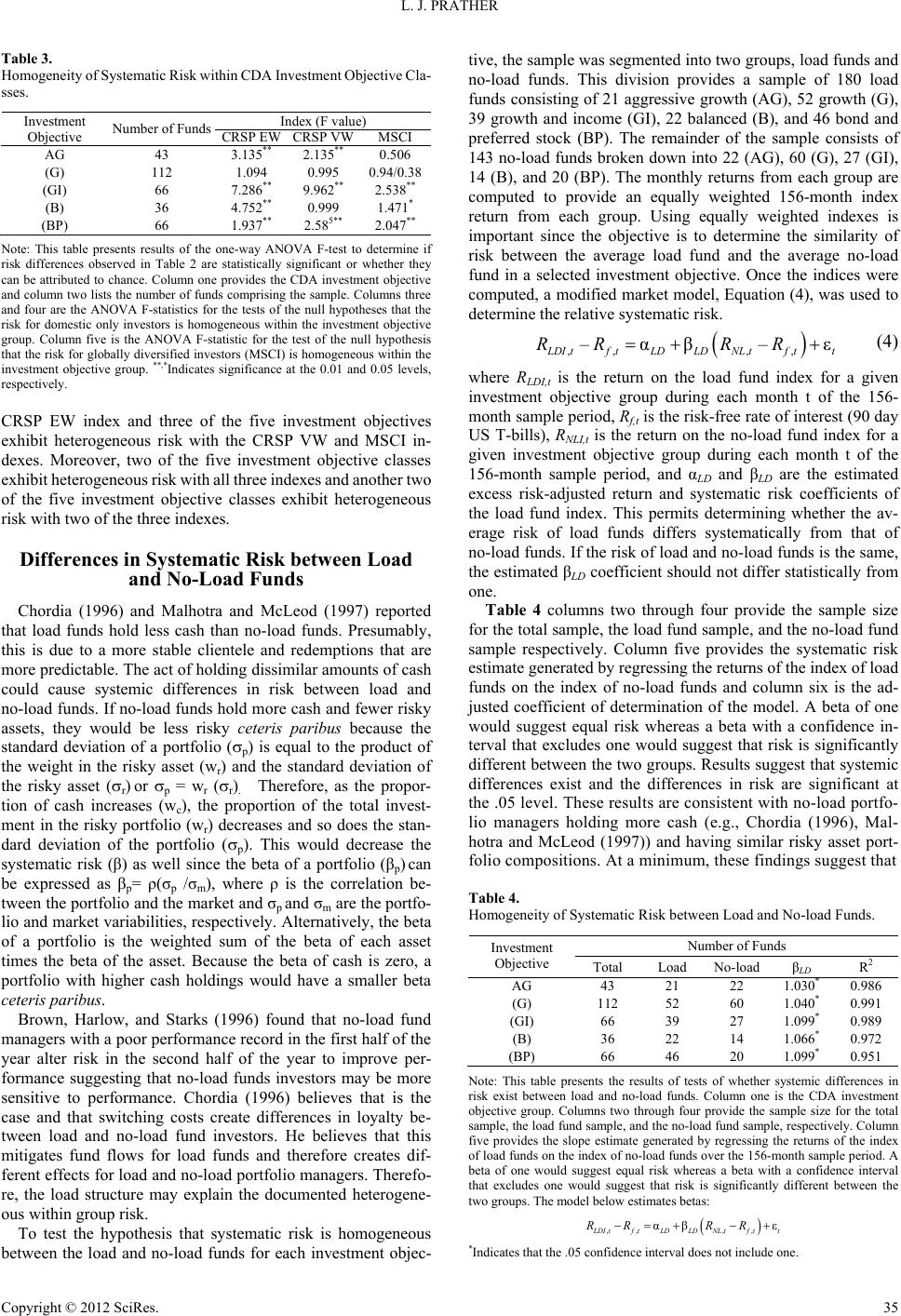
Table 3.
Homogeneity of Systematic Risk within CDA Investment Objective Cla-
Index (F value)
sses.
Investment Number of Funds CRSP EWMSCI
Objective CRSP VW
AG 43 3.135** 2.135** 0.506
(G) 112 1.094 0.995 0.94/0.38
(GI) 66 7.286** 9.962** 2.538**
(B) 36 4.752** 0.999 1.471*
(BP) 66 1.937** 2.585** 2.047**
Note: T presents reshe onOVto df
be
his tableults of te-way ANA F-test etermine i
risk differences observed in Table 2 are statistically significant or whether they
can be attributed to chance. Column one provides the CDA investment objective
and column two lists the number of funds comprising the sample. Columns three
and four are the ANOVA F-statistics for the tests of the null hypotheses that the
risk for domestic only investors is homogeneous within the investment objective
group. Column five is the ANOVA F-statistic for the test of the null hypothesis
that the risk for globally diversified investors (MSCI) is homogeneous within the
investment objective group. **,*Indicates significance at the 0.01 and 0.05 levels,
respectively.
CRSP EW index and three of the five investment objectives
exhibit heterogeneous risk with the CRSP VW and MSCI in-
dexes. Moreover, two of the five investment objective classes
exhibit heterogeneous risk with all three indexes and another two
of the five investment objective classes exhibit heterogeneous
risk with two of the three indexes.
Differences in Systematic Risk between Load
and No-Load Funds
Chordia (1996) and Malhotra and McLeod (1997) reported
that load funds hold less cash than no-load funds. Presumably,
this is due to a more stable clientele and redemptions that are
more predictable. The act of holding dissimilar amounts of cash
could cause systemic differences in risk between load and
no-load funds. If no-load funds hold more cash and fewer risky
assets, they would be less risky ceteris paribus because the
standard deviation of a portfolio (p) is equal to the product of
the weight in the risky asset (wr) and the standard deviation of
the risky asset (r) or p = wr (r). Therefore, as the propor-
tion of cash increases (wc), the proportion of the total invest-
ment in the risky portfolio (wr) decreases and so does the stan-
dard deviation of the portfolio (p). This would decrease the
systematic risk (β) as well since the beta of a portfolio (βp) can
be expressed as βp= ρ(σp /σm), where ρ is the correlation be-
tween the portfolio and the market and σp
and σm are the portfo-
lio and market variabilities, respectively. Alternatively, the beta
of a portfolio is the weighted sum of the beta of each asset
times the beta of the asset. Because the beta of cash is zero, a
portfolio with higher cash holdings would have a smaller beta
ceteris paribus.
Brown, Harlow, and Starks (1996) found that no-load fund
managers with a poor performance record in the first half of the
year alter risk in the second half of the year to improve per-
formance suggesting that no-load funds investors may be more
sensitive to performance. Chordia (1996) believes that is the
case and that switching costs create differences in loyalty be-
tween load and no-load fund investors. He believes that this
mitigates fund flows for load funds and therefore creates dif-
ferent effects for load and no-load portfolio managers. Therefo-
re, the load structure may explain the documented heterogene-
ous within group risk.
To test the hypothesis that systematic risk is homogeneous
tween the load and no-load funds for each investment objec-
tive, the sample was segmented into two groups, load funds and
no-load funds. This division provides a sample of 180 load
funds consisting of 21 aggressive growth (AG), 52 growth (G),
39 growth and income (GI), 22 balanced (B), and 46 bond and
preferred stock (BP). The remainder of the sample consists of
143 no-load funds broken down into 22 (AG), 60 (G), 27 (GI),
14 (B), and 20 (BP). The monthly returns from each group are
computed to provide an equally weighted 156-month index
return from each group. Using equally weighted indexes is
important since the objective is to determine the similarity of
risk between the average load fund and the average no-load
fund in a selected investment objective. Once the indices were
computed, a modified market model, Equation (4), was used to
determine the relative systematic risk.
–αβ
,, ,,
–ε
DItf tLDLDNLtf tt
RRR R
(4)
where RLDI,t is the return on the load fund index for
ble 4 columns two through four provide the sample size
fo
able 4.
ity of Systematic Risk between Load and No-load Funds.
a given
investment objective group during each month t of the 156-
month sample period, Rf,t is the risk-free rate of interest (90 day
US T-bills), RNLI,t is the return on the no-load fund index for a
given investment objective group during each month t of the
156-month sample period, and αLD and βLD are the estimated
excess risk-adjusted return and systematic risk coefficients of
the load fund index. This permits determining whether the av-
erage risk of load funds differs systematically from that of
no-load funds. If the risk of load and no-load funds is the same,
the estimated βLD coefficient should not differ statistically from
one.
Ta
r the total sample, the load fund sample, and the no-load fund
sample respectively. Column five provides the systematic risk
estimate generated by regressing the returns of the index of load
funds on the index of no-load funds and column six is the ad-
justed coefficient of determination of the model. A beta of one
would suggest equal risk whereas a beta with a confidence in-
terval that excludes one would suggest that risk is significantly
different between the two groups. Results suggest that systemic
differences exist and the differences in risk are significant at
the .05 level. These results are consistent with no-load portfo-
lio managers holding more cash (e.g., Chordia (1996), Mal-
hotra and McLeod (1997)) and having similar risky asset port-
folio compositions. At a minimum, these findings suggest that
T
Homogene
Number of Funds
Investment
Objective Total LoadLD R
2 No-load β
AG 43 21 22 1. 0.030*986
(G) 112 52 60 1.040* 0.991
(GI) 66 39 27 1.099* 0.989
(B) 36 22 14 1.066* 0.972
(BP) 66 46 20 1.099* 0.951
Note: Tle presentltsests of whether siffhis tabs the resu of tystemic derences in
risk exist between load and no-load funds. Column one is the CDA investment
objective group. Columns two through four provide the sample size for the total
sample, the load fund sample, and the no-load fund sample, respectively. Column
five provides the slope estimate generated by regressing the returns of the index
of load funds on the index of no-load funds over the 156-month sample period. A
beta of one would suggest equal risk whereas a beta with a confidence interval
that excludes one would suggest that risk is significantly different between the
two groups. The model below estimates betas:
αβ
,, ,,
ε
DItf tLDLDNLtf tt
RRR R
*Indicates that the .05 confidence interval does not include oe. n
Copyright © 2012 SciRes. 35


