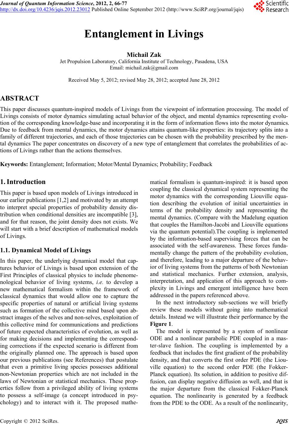
Journal of Quantum Information Science, 2012, 2, 66-77
http://dx.doi.org/10.4236/jqis.2012.23012 Published Online September 2012 (http://www.SciRP.org/journal/jqis)
Entanglement in Livings
Michail Zak
Jet Propulsion Laboratory, California Institute of Technology, Pasadena, USA
Received May 5, 2012; revised May 28, 2012; accepted June 28, 2012
ABSTRACT
This paper discusses quantum-inspired models of Livings from the viewpoint of information processing. The model of
Livings consists of motor dynamics simulating actual behavior of the object, and mental dynamics representing evolu-
tion of the corresponding knowledge-base and incorporating it in the form of information flows into the motor dynamics.
Due to feedback from mental dynamics, the motor dynamics attains quantum-like properties: its trajectory splits into a
family of different trajectories, and each of those trajectories can be chosen with the probability prescribed by the men-
tal dynamics The paper concentrates on discovery of a new type of entanglement that correlates the probabilities of ac-
tions of Livings rather than the actions themselves.
Keywords: Entanglement; Information; Motor/Mental Dynamics; Probability; Feedback
1. Introduction
This paper is based upon models of Livings introduced in
our earlier publications [1,2] and motivated by an attempt
to interpret special properties of probability density dis-
tribution when conditional densities are incompatible [3],
and for that reason, the joint density does not exists. We
will start with a brief description of mathematical models
of Livings.
1.1. Dynamical Model of Livings
In this paper, the underlying dynamical model that cap-
tures behavior of Livings is based upon extension of the
First Principles of classical physics to include phenome-
nological behavior of living systems, i.e. to develop a
new mathematical formalism within the framework of
classical dynamics that would allow one to capture the
specific properties of natural or artificial living systems
such as formation of the collective mind based upon ab-
stract images of the selves and non-selves, exploitation of
this collective mind for communications and predictions
of future expected characteristics of evolution, as well as
for making decisions and implementing the correspond-
ing corrections if the expected scenario is different from
the originally planned one. The approach is based upon
our previous publications (see References) that postulate
that even a primitive living species possesses additional
non-Newtonian properties which are not included in the
laws of Newtonian or statistical mechanics. These prop-
erties follow from a privileged ability of living systems
to possess a self-image (a concept introduced in psy-
chology) and to interact with it. The proposed mathe-
matical formalism is quantum-inspired: it is based upon
coupling the classical dynamical system representing the
motor dynamics with the corresponding Liouville equa-
tion describing the evolution of initial uncertainties in
terms of the probability density and representing the
mental dynamics. (Compare with the Madelung equation
that couples the Hamilton-Jacobi and Liouville equations
via the quantum potential).The coupling is implemented
by the information-based supervising forces that can be
associated with the self-awareness. These forces funda-
mentally change the pattern of the probability evolution,
and therefore, leading to a major departure of the behav-
ior of living systems from the patterns of both Newtonian
and statistical mechanics. Further extension, analysis,
interpretation, and application of this approach to com-
plexity in Livings and emergent intelligence have been
addressed in the papers referenced above.
In the next introductory sub-sections we will briefly
review these models without going into mathematical
details. Instead we will illustrate their performance by the
Figure 1.
The model is represented by a system of nonlinear
ODE and a nonlinear parabolic PDE coupled in a mas-
ter-slave fashion. The coupling is implemented by a
feedback that includes the first gradient of the probability
density, and that converts the first order PDE (the Liou-
ville equation) to the second order PDE (the Fokker-
Planck equation). Its solution, in addition to positive dif-
fusion, can display negative diffusion as well, and that is
the major departure from the classical Fokker-Planck
equation. The nonlinearity is generated by a feedback
from the PDE to the ODE. As a result of the nonlinearity,
C
opyright © 2012 SciRes. JQIS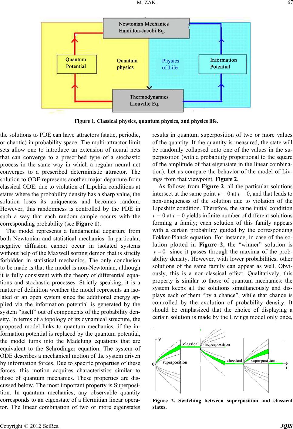

M. ZAK 67
Figure 1. Classical physics, quantum physics, and physics life.
the solutions to PDE can have attractors (static, periodic,
or chaotic) in probability space. The multi-attractor limit
sets allow one to introduce an extension of neural nets
that can converge to a prescribed type of a stochastic
process in the same way in which a regular neural net
converges to a prescribed deterministic attractor. The
solution to ODE represents another major departure from
classical ODE: due to violation of Lipchitz conditions at
states where the probability density has a sharp value, the
solution loses its uniqueness and becomes random.
However, this randomness is controlled by the PDE in
such a way that each random sample occurs with the
corresponding probability (see Figure 1).
The model represents a fundamental departure from
both Newtonian and statistical mechanics. In particular,
negative diffusion cannot occur in isolated systems
without help of the Maxwell sorting demon that is strictly
forbidden in statistical mechanics. The only conclusion
to be made is that the model is non-Newtonian, although
it is fully consistent with the theory of differential equa-
tions and stochastic processes. Strictly speaking, it is a
matter of definition weather the model represents an iso-
lated or an open system since the additional energy ap-
plied via the information potential is generated by the
system “itself” out of components of the probability den-
sity. In terms of a topology of its dynamical structure, the
proposed model links to quantum mechanics: if the in-
formation potential is replaced by the quantum potential,
the model turns into the Madelung equations that are
equivalent to the Schrödinger equation. The system of
ODE describes a mechanical motion of the system driven
by information forces. Due to specific properties of these
forces, this motion acquires characteristics similar to
those of quantum mechanics. These properties are dis-
cussed below. The most important property is Superposi-
tion. In quantum mechanics, any observable quantity
corresponds to an eigenstate of a Hermitian linear opera-
tor. The linear combination of two or more eigenstates
results in quantum superposition of two or more values
of the quantity. If the quantity is measured, the state will
be randomly collapsed onto one of the values in the su-
perposition (with a probability proportional to the square
of the amplitude of that eigenstate in the linear combina-
tion). Let us compare the behavior of the model of Liv-
ings from that viewpoint, Figure 2.
As follows from Figure 2, all the particular solutions
intersect at the same point v = 0 at t = 0, and that leads to
non-uniqueness of the solution due to violation of the
Lipcshitz condition. Therefore, the same initial condition
v = 0 at t = 0 yields infinite number of different solutions
forming a family; each solution of this family appears
with a certain probability guided by the corresponding
Fokker-Planck equation. For instance, in case of the so-
lution plotted in Figure 2, the “winner” solution is
0v

since it passes through the maxima of the prob-
ability density. However, with lower probabilities, other
solutions of the same family can appear as well. Obvi-
ously, this is a non-classical effect. Qualitatively, this
property is similar to those of quantum mechanics: the
system keeps all the solutions simultaneously and dis-
plays each of them “by a chance”, while that chance is
controlled by the evolution of probability density. It
should be emphasized that the choice of displaying a
certain solution is made by the Livings model only once,
Figure 2. Switching between superposition and classical
states.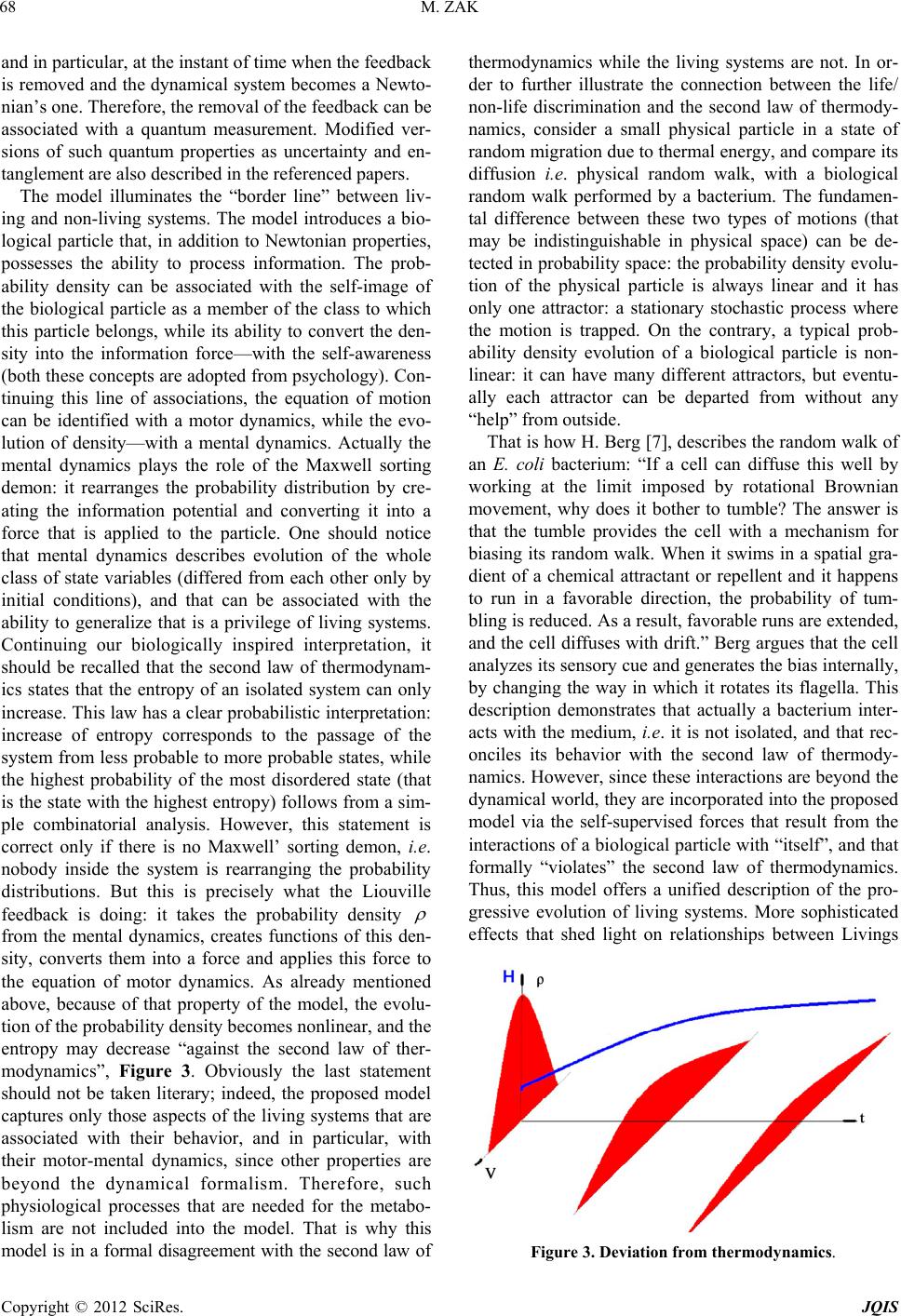

M. ZAK
68
and in particular, at the instant of time when the feedback
is removed and the dynamical system becomes a Newto-
nian’s one. Therefore, the removal of the feedback can be
associated with a quantum measurement. Modified ver-
sions of such quantum properties as uncertainty and en-
tanglement are also described in the referenced papers.
The model illuminates the “border line” between liv-
ing and non-living systems. The model introduces a bio-
logical particle that, in addition to Newtonian properties,
possesses the ability to process information. The prob-
ability density can be associated with the self-image of
the biological particle as a member of the class to which
this particle belongs, while its ability to convert the den-
sity into the information force—with the self-awareness
(both these concepts are adopted from psychology). Con-
tinuing this line of associations, the equation of motion
can be identified with a motor dynamics, while the evo-
lution of density—with a mental dynamics. Actually the
mental dynamics plays the role of the Maxwell sorting
demon: it rearranges the probability distribution by cre-
ating the information potential and converting it into a
force that is applied to the particle. One should notice
that mental dynamics describes evolution of the whole
class of state variables (differed from each other only by
initial conditions), and that can be associated with the
ability to generalize that is a privilege of living systems.
Continuing our biologically inspired interpretation, it
should be recalled that the second law of thermodynam-
ics states that the entropy of an isolated system can only
increase. This law has a clear probabilistic interpretation:
increase of entropy corresponds to the passage of the
system from less probable to more probable states, while
the highest probability of the most disordered state (that
is the state with the highest entropy) follows from a sim-
ple combinatorial analysis. However, this statement is
correct only if there is no Maxwell’ sorting demon, i.e.
nobody inside the system is rearranging the probability
distributions. But this is precisely what the Liouville
feedback is doing: it takes the probability density

from the mental dynamics, creates functions of this den-
sity, converts them into a force and applies this force to
the equation of motor dynamics. As already mentioned
above, because of that property of the model, the evolu-
tion of the probability density becomes nonlinear, and the
entropy may decrease “against the second law of ther-
modynamics”, Figure 3. Obviously the last statement
should not be taken literary; indeed, the proposed model
captures only those aspects of the living systems that are
associated with their behavior, and in particular, with
their motor-mental dynamics, since other properties are
beyond the dynamical formalism. Therefore, such
physiological processes that are needed for the metabo-
lism are not included into the model. That is why this
model is in a formal disagreement with the second law of
thermodynamics while the living systems are not. In or-
der to further illustrate the connection between the life/
non-life discrimination and the second law of thermody-
namics, consider a small physical particle in a state of
random migration due to thermal energy, and compare its
diffusion i.e. physical random walk, with a biological
random walk performed by a bacterium. The fundamen-
tal difference between these two types of motions (that
may be indistinguishable in physical space) can be de-
tected in probability space: the probability density evolu-
tion of the physical particle is always linear and it has
only one attractor: a stationary stochastic process where
the motion is trapped. On the contrary, a typical prob-
ability density evolution of a biological particle is non-
linear: it can have many different attractors, but eventu-
ally each attractor can be departed from without any
“help” from outside.
That is how H. Berg [7], describes the random walk of
an E. coli bacterium: “If a cell can diffuse this well by
working at the limit imposed by rotational Brownian
movement, why does it bother to tumble? The answer is
that the tumble provides the cell with a mechanism for
biasing its random walk. When it swims in a spatial gra-
dient of a chemical attractant or repellent and it happens
to run in a favorable direction, the probability of tum-
bling is reduced. As a result, favorable runs are extended,
and the cell diffuses with drift.” Berg argues that the cell
analyzes its sensory cue and generates the bias internally,
by changing the way in which it rotates its flagella. This
description demonstrates that actually a bacterium inter-
acts with the medium, i.e. it is not isolated, and that rec-
onciles its behavior with the second law of thermody-
namics. However, since these interactions are beyond the
dynamical world, they are incorporated into the proposed
model via the self-supervised forces that result from the
interactions of a biological particle with “itself”, and that
formally “violates” the second law of thermodynamics.
Thus, this model offers a unified description of the pro-
gressive evolution of living systems. More sophisticated
effects that shed light on relationships between Livings
Figure 3. Deviation from thermodynamics.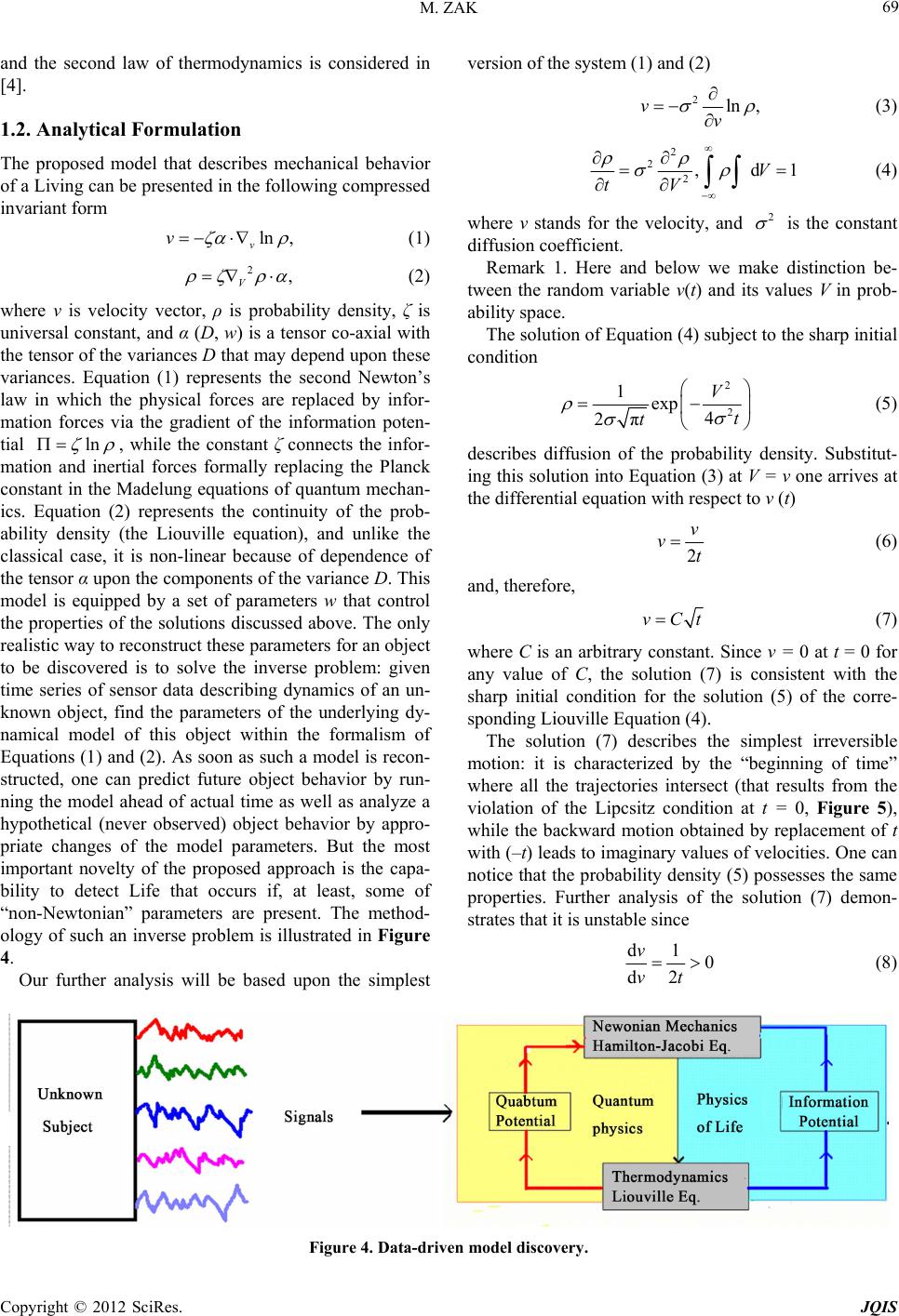

M. ZAK
69
and the second law of thermodynamics is considered in
[4].
1.2. Analytical Formulation
The proposed model that describes mechanical behavior
of a Living can be presented in the following compressed
invariant form
ln ,
v
v

    (1)
2,
V

  (2)
where ν is velocity vector, ρ is probability density, ζ is
universal constant, and α (D, w) is a tensor co-axial with
the tensor of the variances D that may depend upon these
variances. Equation (1) represents the second Newton’s
law in which the physical forces are replaced by infor-
mation forces via the gradient of the information poten-
tial ln

  , while the constant ζ connects the infor-
mation and inertial forces formally replacing the Planck
constant in the Madelung equations of quantum mechan-
ics. Equation (2) represents the continuity of the prob-
ability density (the Liouville equation), and unlike the
classical case, it is non-linear because of dependence of
the tensor α upon the components of the variance D. This
model is equipped by a set of parameters w that control
the properties of the solutions discussed above. The only
realistic way to reconstruct these parameters for an object
to be discovered is to solve the inverse problem: given
time series of sensor data describing dynamics of an un-
known object, find the parameters of the underlying dy-
namical model of this object within the formalism of
Equations (1) and (2). As soon as such a model is recon-
structed, one can predict future object behavior by run-
ning the model ahead of actual time as well as analyze a
hypothetical (never observed) object behavior by appro-
priate changes of the model parameters. But the most
important novelty of the proposed approach is the capa-
bility to detect Life that occurs if, at least, some of
“non-Newtonian” parameters are present. The method-
ology of such an inverse problem is illustrated in Figure
4.
Our further analysis will be based upon the simplest
version of the system (1) and (2)
2ln ,vv


  (3)
2
2
2,dV
tV




 1


 (4)
where v stands for the velocity, and 2

is the constant
diffusion coefficient.
Remark 1. Here and below we make distinction be-
tween the random variable v(t) and its values V in prob-
ability space.
The solution of Equation (4) subject to the sharp initial
condition
2
2
1exp 4
2π
V
t
t







(5)
describes diffusion of the probability density. Substitut-
ing this solution into Equation (3) at V = v one arrives at
the differential equation with respect to v (t)
2
v
vt  (6)
and, therefore,
vCt (7)
where C is an arbitrary constant. Since v = 0 at t = 0 for
any value of C, the solution (7) is consistent with the
sharp initial condition for the solution (5) of the corre-
sponding Liouville Equation (4).
The solution (7) describes the simplest irreversible
motion: it is characterized by the “beginning of time”
where all the trajectories intersect (that results from the
violation of the Lipcsitz condition at t = 0, Figure 5),
while the backward motion obtained by replacement of t
with (–t) leads to imaginary values of velocities. One can
notice that the probability density (5) possesses the same
properties. Further analysis of the solution (7) demon-
strates that it is unstable since
d1
0
d2
v
vt

 (8)
Figure 4. Data-driven model discovery.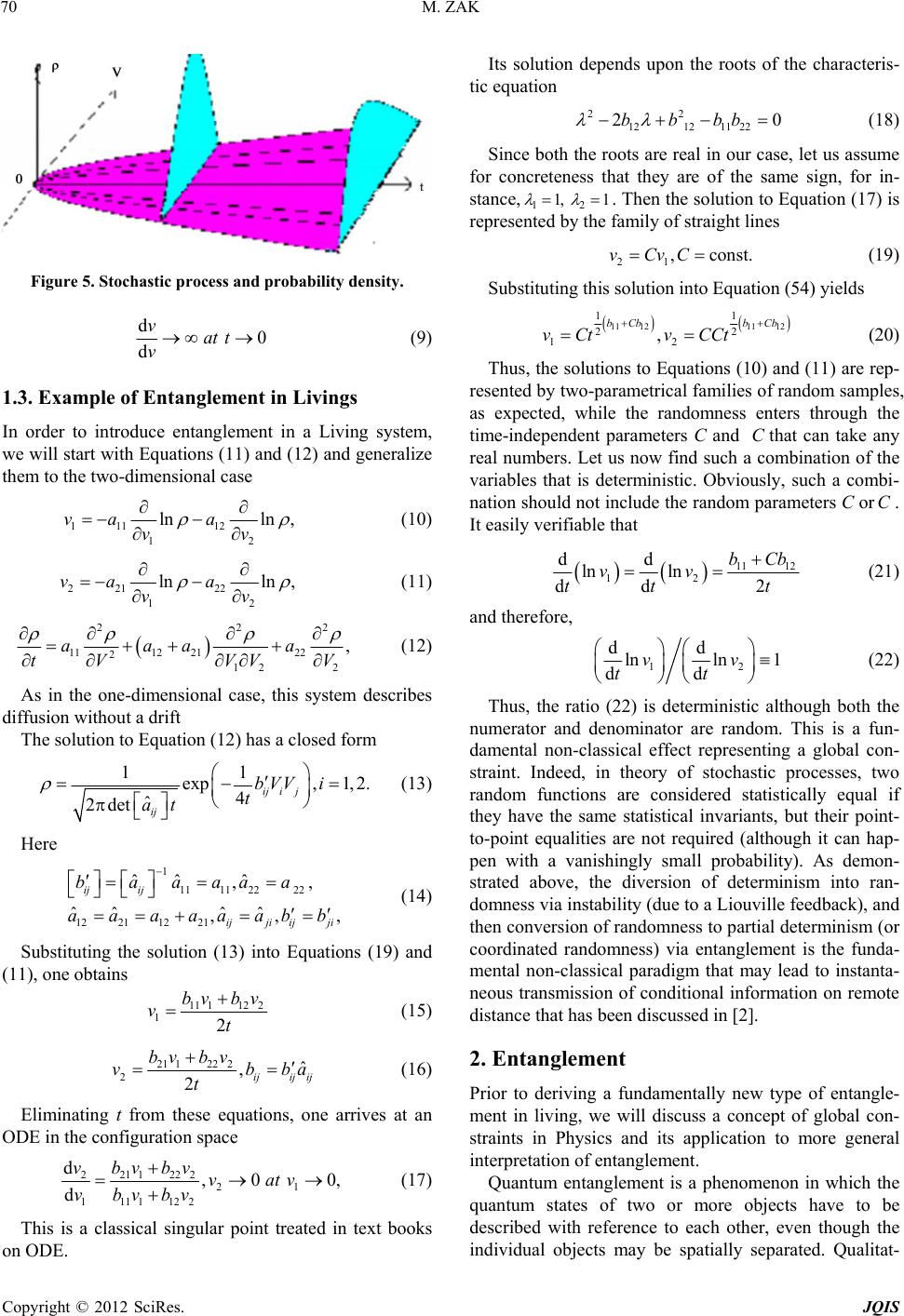

M. ZAK
70
Figure 5. Stochastic process and probability density.
d 0
d
vat t
v (9)
1.3. Example of Entanglement in Livings
In order to introduce entanglement in a Living system,
we will start with Equations (11) and (12) and generalize
them to the two-dimensional case
111 12
12
lnln ,va a
vv



 

(10)
221 22
12
lnln ,va a
vv



 

(11)

22
1112 2122
2
12 2
,aaa a
tVV V
2
V

  
 
 


(12)
As in the one-dimensional case, this system describes
diffusion without a drift
The solution to Equation (12) has a closed form
11
exp,1, 2.
4
ˆ
2det
ij ij
ij
bVVi
t
at









,
(13)
Here
1
1111 2222
1221 12 21
ˆˆ ˆ
,,
ˆˆˆˆ
,,
ij ij
ijji ijji
baaaaa
aaaaaabb

 


  (14)
Substituting the solution (13) into Equations (19) and
(11), one obtains
11 1122
12
bv bv
vt

 (15)
21 1222
2ˆ
,
2ijij ij
bv bv
vb
t

ba (16)
Eliminating t from these equations, one arrives at an
ODE in the configuration space
2211222
21
1111122
d,0
d
vbvbv
vatv
vbvbv


0,
(17)
This is a classical singular point treated in text books
on ODE.
Its solution depends upon the roots of the characteris-
tic equation
22
121211 22
20bbbb 

  (18)
Since both the roots are real in our case, let us assume
for concreteness that they are of the same sign, for in-
stance, 12
1, 1 

. Then the solution to Equation (17) is
represented by the family of straight lines
21
,consvCvCt. (19)
Substituting this solution into Equation (54) yields
 
(20)
11 1211 12
11
22
12
,
bCb bCb
v CtvCCt


Thus, the solutions to Equations (10) and (11) are rep-
resented by two-parametrical families of random samples,
as expected, while the randomness enters through the
time-independent parameters C and that can take any
real numbers. Let us now find such a combination of the
variables that is deterministic. Obviously, such a combi-
nation should not include the random parameters C or C.
It easily verifiable that
C
 
11 12
12
dd
ln ln
dd 2
bCb
vv
tt t

 (21)
and therefore,
12
dd
lnln 1
dd
vv
tt




(22)
Thus, the ratio (22) is deterministic although both the
numerator and denominator are random. This is a fun-
damental non-classical effect representing a global con-
straint. Indeed, in theory of stochastic processes, two
random functions are considered statistically equal if
they have the same statistical invariants, but their point-
to-point equalities are not required (although it can hap-
pen with a vanishingly small probability). As demon-
strated above, the diversion of determinism into ran-
domness via instability (due to a Liouville feedback), and
then conversion of randomness to partial determinism (or
coordinated randomness) via entanglement is the funda-
mental non-classical paradigm that may lead to instanta-
neous transmission of conditional information on remote
distance that has been discussed in [2].
2. Entanglement
Prior to deriving a fundamentally new type of entangle-
ment in living, we will discuss a concept of global con-
straints in Physics and its application to more general
interpretation of entanglement.
Quantum entanglement is a phenomenon in which the
quantum states of two or more objects have to be
described with reference to each other, even though the
individual objects may be spatially separated. Qualitat-

M. ZAK 71
ively similar effect has been demonstrated in living
systems: as follows from the example considered in the
previous section, the diversion of determinism into ran-
domness via instability (due to a Liouville feedback), and
then conversion of randomness to partial determinism (or
coordinated randomness) via entanglement is the funda-
mental non-classical paradigm that may lead to instanta-
neous transmission of conditional information on remote
distance [2]. In this connection, it is reasonable to make
some comments about non-locality in physics. As al-
ready mentioned above, the living systems and quantum
systems have similar topology (see Figure 1). In this
section, we will analyze the similarities in terms of en-
tanglement that follow from this topology.
2.1. Criteria for Non-Local Interactions
Based upon analysis of all the known interactions in the
Universe and defining them as local, one can formulate
the following criteria of non-local interactions: they are
not mediated by another entity, such as a particle or field;
their actions are not limited by the speed of light; the
strength of the interactions does not drop off with dis-
tance. All of these criteria lead us to the concept of the
global constraint as a starting point.
2.2. Global Constraints in Physics
It should be recalled that the concept of a global con-
straint is one of the main attribute of Newtonian me-
chanics. It includes such idealizations as a rigid body, an
incompressible fluid, an inextensible string and a mem-
brane, a non-slip rolling of a rigid ball over a rigid body,
etc. All of those idealizations introduce geometrical or
kinematical restrictions to positions or velocities of parti-
cles and provide “instantaneous” speed of propagation of
disturbances. Let us discuss the role of the reactions of
these constraints. One should recall that in an income-
pressible fluid, the reaction of the global constraint
(expressing non-negative divergence of the
velocity v) is a non-negative pressure ; in inexten-
sible flexible (one- or two-dimensional) bodies, the reac-
tion of the global constraint ij ij
0v 
0p
,
0
g
g i, j = 1, 2 (ex-
pressing that the components of the metric tensor cannot
exceed their initial values) is a non-negative stress tensor
0
ij

, i, j = 1, 2. It should be noticed that all the known
forces in physics (the gravitational, the electromagnetic,
the strong and the weak nuclear forces) are local. How-
ever, the reactions of the global constraints listed above
do not belong to any of these local forces, and therefore,
they are non-local. Although these reactions are being
successfully applied for engineering approximations of
theoretical physics, one cannot relate them to the origin
of entanglement since they are result of idealization that
ignores the discrete nature of the matter. However, there
is another type of the global constraint in physics: the
normalization constraint (see Equation (4)). This con-
straint is fundamentally different from those listed above
for two reasons. Firstly, it is not an idealization, and
therefore, it cannot be removed by taking into account
more subtle properties of matter such as elasticity, com-
pressibility, discrete structure, etc. Secondly, it imposes
restrictions not upon positions or velocities of particles,
but upon the probabilities of their positions or velocities,
and that is where the entanglement comes from. Indeed,
if the Liouville equation is coupled with equations of
motion as in quantum mechanics, the normalization con-
dition imposes a global constraint upon the state vari-
ables, and that is the origin of quantum entanglement. In
quantum physics, the reactions of the normalization con-
straints can be associated with the energy eigenvalues
that play the role of the Lagrange multipliers in the con-
ditional extremum formulation of the Schrödinger equa-
tion [5]. In living systems, the Liouville equation is also
coupled with equations of motion (although the feedback
is different). And that is why the origin of entanglement
in living systems is the same as in quantum mechanics.
2.3. Speed of Action Propagation
Further illumination of the concept of quantum entan-
glement follows from comparison of quantum and New-
tonian systems. Such a comparison is convenient to per-
form in terms of the Madelung version of the Schrödinger
equation:
0S
tm
 




(23)

22
20
2
SSV
tm





 
 (24)
Here

and S are the components of the wave func-
tion /iS e  , and is the Planck constant divided
by . The Newtonian mechanics (), in terms of
the S and
2π0

as state variables, is of a hyperbolic type,
and therefore, any discontinuity propagates with the fi-
nite speed S/m, i.e. the Newtonian systems do not have
non-localities. But the quantum mechanics (0

) is of a
parabolic type. This means that any disturbance of S or

in one point of space instantaneously transmitted to
the whole space, and this is the mathematical origin of
non-locality. But is this a unique property of quantum
evolution? Obviously, it is not. Any parabolic equation
(such as Navier-Stokes equations or Fokker-Planck equa-
tion) has exactly the same non-local properties. However,
the difference between the quantum and classical non-
localities is in their physical interpretation. Indeed, the
Navier-Stokes equations are derived from simple laws of
Newtonian mechanics, and that is why a physical inter-

M. ZAK
72
pretation of non-locality is very simple: If a fluid is in-
compressible, then the pressure plays the role of a reac-
tion to the geometrical constraint , and it is
transmitted instantaneously from one point to the whole
space (the Pascal law). One can argue that the incom-
pressible fluid is an idealization, and that is true. How-
ever, it does not change our point: Such a model has a lot
of engineering applications, and its non-locality is well
understood. The situation is different in quantum me-
chanics since the Schrodinger equation has never been
derived from Newtonian mechanics: It has been postu-
lated. In addition to that, the solutions of the Schrodinger
equation are random, while the origin of the randomness
does not follow from the Schrodinger formalism. That is
why the physical origin of the same mathematical phe-
nomenon cannot be reduced to simpler concepts such as
“forces”: It should be accepted as an attribute of the
Schrodinger equation.
0v 
Let us turn now to the living systems. The formal dif-
ference between them and quantum systems is in a feed-
back from the Liouville equation to equations of motion:
the gradient of the quantum potential is replaced by the
information forces, while the equations of motion are
written in the form of the second Newton’s law rather
than in the Hamilton-Jacoby form. In this paper, we have
considered information forces that turn the corresponding
Liouville equation into the Fokker-Planck equation
which is parabolic, and therefore, all the changes of the
probability density propagates instantaneously as in the
quantum systems. Thus, both quantum systems and liv-
ing systems possess the same non-locality: instantaneous
propagation of changes in the probability density, and
this is due to similar topology of their dynamical struc-
ture, and in particular, due to a feedback from the Liou-
ville equation.
2.4. Origin of Randomness in Physics
Since entanglement in quantum systems as well as in
living systems is exposed via instantaneous propagation
of changes in the probability density, it is relevant to ask
what is the origin of randomness in physics. The concept
of randomness has a long history. Its philosophical as-
pects first were raised by Aristotle, while the math-
ematic- cal foundations were introduced and discussed
much later by Henry Poincare who wrote: “A very slight
cause, which escapes us, determines a considerable effect
which we cannot help seeing, and then we say this effect
is due to chance.” Actually Poincare suggested that the
origin of randomness in physics is the dynamical insta-
bility, and this viewpoint has been corroborated by the-
ory of turbulence and chaos. However, the theory of dy-
namical stability developed by Poincare and Lyapunov
revealed the main flaw of physics: its fundamental laws
do not discriminate between stable and unstable motions.
But unstable motions cannot be realized and observed,
and therefore, a special mathematical analysis must be
added to found out the existence and observability of the
motion under consideration. However, then another ques-
tion can be raised: why turbulence as a postinstability
version of an underlying laminar flow can be observed
and measured? In order to answer this question, we have
to notice that the concept of stability is an attribute of
mathematics rather than physics, and in mathematical
formalism, stability must be referred to the correspond-
ing class of functions. For example: a laminar motion
with sub-critical Reynolds number is stable in the class
of deterministic functions. Similarly, a turbulent motion
is stable in the class of random functions. Thus the same
physical phenomenon can be unstable in one class of
functions, but stable in another, enlarged class of func-
tions.
Thus, we are ready now to the following conclusion:
any stochastic process in Newtonian dynamics describes
the physical phenomenon that is unstable in the class of
the deterministic functions.
This elegant union of physics and mathematics has
been disturbed by the discovery of quantum mechanics
that complicated the situation: Quantum physicists claim
that quantum randomness is the “true” randomness unlike
the “deterministic” randomness of chaos and turbulence.
Richard Feynman in his “Lectures on Physics” stated that
randomness in quantum mechanics in postulated, and
that closes any discussions about its origin. However,
recent result disproved existence of the “true” random-
ness. Indeed, as shown in [2], the origin of randomness in
quantum mechanics can be traced down to instability
generated by quantum potential at the point of departure
from a deterministic state if for dynamical analysis one
transfer from the Shrodinger to the Madelung equation.
(For details see [2]). As demonstrated there, the instabil-
ity triggered by failure of the Lipchitz condition splits the
solution into a continuous set of random samples repre-
senting a “bridge” to quantum world. Hence, now we can
state that any stochastic process in physics describes the
physical phenomenon that is unstable in the class of the
deterministic functions. Actually this statement can be
used as a definition of randomness in physics. Finally
one may ask why the instability discussed above has not
been detected in the Schrödinger equation. The answer is
simple if one recalls that stability analysis is based upon
a departure from the basic state into a perturbed state,
and such departure requires an expansion of the basic
space. However, Schrödinger and Madelung equations in
the expanded spaces are not necessarily equivalent any
more, and that confirm the fact that stability is not an
invariant of a dynamical system: it can depend upon the
definition of a distance between the basic and perturbed

M. ZAK 73
motions, and these definitions are different for Hilbert
and physical spaces.
3. Partial Entanglement in Livings
In this section we introduce a new, more sophisticated
entanglement that does not exists in quantum mechanics,
but can be found in Livings. This finding is based upon
existence of incompatible stochastic processes that are
considered below.
3.1. Incompatible Stochastic Processes
Classical probability theory defines conditional proba-
bility densities based upon the existence of a joint prob-
ability density. However, one can construct correlated
stochastic processes that are represented only by condi-
tional densities since a joint probability density does not
exist. For that purpose, consider two coupled Langevin
equations [6].

11121
x
gxLt (25)
 
22212
x
gxLt (26)
where the Langevin forces


1
Ltand satisfy the
conditions

2
Lt
  
0, 2
iiiii
LtLtLtgt t 



 (27)
Then the joint probability density

12
,
X
X  de-
scribing uncertainties in values of the random variables
1
x
and 2
x
evolves according to the following Fokker-
Planck equation
 
22
22
112221
22
12
gXg X
t
X
X





(28)
Let us now modify Equations (25) and (26) as follow-
ing


2*
11121
x
gxLt (29)


2*
22212
x
gxLt (30)
where *
1
x
and 2
*
x
are fixed values of 1
x
and 2
x
that
play role of parameters in Equations (29) and (30), re-
spectively. Now the uncertainties of 1
x
and 2
x
are char-
acterized by conditional probability densities


11
|2
X
X 
and 1

|

22
X
X  while each of these densities is gov-
erned by its own Fokker-Planck equation

2
2 1
11 22
1
gX
t
1
X





(31)

2
2
2
22 1
2
gX
tX
2





(32)
The solutions of these equations subject to sharp initial
conditions




,, ,1,2.
(33)
iiii i
XtXtXXi 


for tt

 read
  

 
11 22
11 2
2
11
2
11 2
1
|
4π
exp(4
XX
gXtt
XX
g
Xtt
 



 

(34)

 

 
2212
22 1
2
22
2
22 1
1
4π
exp4
XX
gXtt
XX
g
Xtt
 







 





(35)
As shown in [3], a joint density for the conditional
densities (34) and (35) exists only in special cases of the
diffusion coefficients g11 and g22 when the conditional
probabilities are compatible. These conditions are
 

11 2
12
122 2 1
|
,ln
|
XX
ink XXX X

 
0


 (36)
Indeed





121 122
212 1
,,
,d,
XX XXX
XX X
d
 









(37)
whence





112
1
221
2
lnln, d
ln,d
XX X
XX
X



 








(38)
and that leads to Equation (36).
Thus, the existence of the join density

12
,
X
X  for
the conditional densities

112
X
X  and


221
X
X 
requires that





2
2112 2
22
12 11 2221
0
44
XXXX
XX gXg X






 

(39)
Obviously the identity (39) holds only for specially
selected functions


11 2
g
X and

22 1
g
X, and there-
fore, existence of the joint density is an exception rather
than a rule.
3.2. Partial Entanglement
In order to prove existence of a new form of entangle-
ment, let us modify the system Equations (10)-(12) as

M. ZAK
74
following:


1112 112
1
lnvav vv
v


 

(40)



2
112 112
11 22
1
VV VV
aV
tV
 

 (41)
 
2221 22
1
lnvav vv
v


 

1
(42)



2
221 221
22 12
2
VV VV
aV
tV
 

 (43)
Since here we do not postulate existence of a joint
density, the system is written in terms of conditional
densities, while Equations (41) and (43) are similar to
Equations (31) and (32). The solutions of these PDE can
be written in the form similar to the solutions (34) and
(35)



 
112
11 2
2
11
11 2
1
4π
exp4
VV
aV tt
VV
aV tt
 





 







(44)

 

 
221
22 1
2
22
11 1
1
4π
exp4
VV
aVtt
VV
aV tt
 





 







(45)
As noticed in the previous sub-section, the existence of
the joint density for the conditional densities

12
,VV 

112
VV 

and

221
VV 

requires that




2
2112 2
12 112221
0
44
VVVV
VVa VaV









 




(46)
In this case, the joint density exists (although its find-
ing is not trivial [3]), and the system (40)-(43) can be
reduced to a system similar to (10)-(12). But here we will
be interested in case when the joint density does not exist.
It is much easier to find such functions



11 222 1
,aVaV
for which the identity (46) does not hold, and we assume
that




2
2112 2
12 112221
0
44
VVVV
VVa VaV









 




(47)
In this case the system (40)-(43) cannot be simplified.
In order to analyze this system in details, let substitute
the solutions (44) and (45) into Equations (40) and (42),
respectively. Then with reference to Equation (6), one
obtains
1
12
v
vt  (48)
2
22
v
vt  (49)
and therefore
11
vCt (50)
22
vCt (51)
It should be recalled that according to the terminology
introduced in Section I, the system (40)-(41) and the sys-
tem (42)-(43) can be considered as dynamical models for
interaction of two communicating agents where Equa-
tions (40) and (42) describes their motor dynamics, and
Equations (41) and (43)—mental dynamics, respectively.
Also it should be reminded that the solutions (50) and
(51) are represented by one-parametrical families of
random samples, as in Equation (7), while the random
ness enters through the time-independent parameters 1
and 2 that can take any real numbers. As follows from
Figure 2, all the particular solutions (50) and (51) inter-
sect at the same point 1,2
C
C
0v

at t = 0, and that leads to
non-uniqueness of the solution due to violation of the
Lipcshitz condition. Therefore, the same initial condition
1,20v

at t = 0 yields infinite number of different solu-
tions forming a family; each solution of this family ap-
pears with a certain probability guided by the corre-
sponding Fokker-Planck Equations (41) and (43), respec-
tively. Similar scenario was described in the Introduction
of this paper. But what unusual in the system (40)-(43) is
correlations: although Equations (41) and (43) are corre-
lated, and therefore, mental dynamics are entangled,
Equations (40) and (42) are not correlated (since they can
be presented in the form of independent Equations (48)
and (49), respectively), and therefore, the motor dynam-
ics are not entangled. This means that in the course of
communications, each agent “selects” a certain pattern of
behavior from the family of solutions (50) and (51) re-
spectively, and these patterns are independent; but the
probabilities of these “selections” are entangled via
Equations (41) and (43). Such sophisticated correlations
cannot be found in physical world, and they obviously
represent a “human touch”. Unlike the entanglement in
system with joint density (such as that in Equations
(10)-(12)) here the agents do not share any deterministic
invariants (compare to Equation (22)). Instead the agents
can communicate via “best guesses” based upon known
probability densities distributions.
In order to quantify the amount of uncertainty due to

M. ZAK 75
incompatibility of the conditional probability densities
(44) and (45), let us introduce a concept of complex
probability [3].

12 1212
,,

,
f
VVaVV ibVV (52)
1112 212 2
11 11
()(, )d(, )d
()()
f
VaVVVibVV
aV ibV

 



V
(53)
22121121
22 22
()(, )d(, )d
()()
f
VaVVVibVV
aV ibV

 



V
(54)
Following the formalism of conditional probabilities,
the conditional density will be defined as
1212 12
1| 2
2222 22
22 22
22 22
22 22
(, )(,)(, )
()() ()
f
VVaVVibVV
ffVaV ibV
aabbabab
i
ab ab






(55)
1212 12
2|1
1111 11
11 11
2222
112 2
(, )(,)(, )
()() ()
f
VVaVVibVV
ffVaVibV
aabbabab
i
aba b






(56)
with the normalization constraint

12
22
12
dd 1ab VV

 

  (57)
This constraint can be enforced by introducing a nor-
malizing multiplier in Equation (52) which will not affect
the conditional densities (55) and (56).
Clearly

12
22,aab and (58)
12
dd 1aV V

 


Now our problem can be reformulated in the following
manner: given two conditional probability densities (44)
and (45), and considering them as real parts of (unknown)
complex densities (55) and (56), find the corresponding
complex joint density (52), and therefore, all the mar-
ginal (53) and (54), as well as the imaginary parts of the
conditional densities. In this case one arrives at two cou-
pled integral equations with respect to two unknowns
and (while the formulations of
,212 , and follow
from Equations (53) and (54)). These equations are

12
,aVV

112
,aVV
 
 

12
,bVV

,VaV

112
,bVV

212
,bVV
 
22 11
112 212
22 22
22 22
,,,
aabbaa bb
VV VV
ab ab



,


(59)
The system (59) is nonlinear, and very little can be
said about general property of its solution without de-
tailed analysis. Omitting such an analysis, let us start
with a trivial case when
b = 0 (60)
In this case the system (59) reduces to the following
two integral equations with respect to one unknown


12
,aVV
 

 

12
112
12 2
12
212
12 2
,
,,
,d
,
,
,d
aVV
VV
aVV V
aVV
VV
aVV V










(61)
This system is overdetermined unless the compatibility
conditions (36) are satisfied.
As known from classical mechanics, the incompatibil-
ity conditions are usually associated with a fundamen-
tally new concept or a physical phenomenon. For in-
stance, incompatibility of velocities in fluid (caused by
non-existence of velocity potential) introduces vorticity
in rotational flows, and incompatibility in strains de-
scribes continua with dislocations. In order to interpret
the incompatibility (36), let us return to the system (59).
Discretizing the functions in Equations (59) and replac-
ing the integrals by the corresponding sums, one reduces
Equations (59) to a system of n algebraic equations with
respect to n unknowns. This means that the system is
closed, and cases when a solution does not exist are ex-
ceptions rather than a rule. Therefore, in most cases, for
any arbitrarily chosen conditional densities, for instant,
for those given by Equations (44) and (45), the system
(59) defines the complex joint density in the form (52).
Now we are ready to discuss a physical meaning of the
imaginary component of the complex probability density.
Firstly, as follows from comparison of Equations (59)
and (61), the imaginary part of the probability density
appears as a response to incompatibility of the condi-
tional probabilities, and therefore, it can be considered as
a “compensation” for the incompatibility. Secondly, as
follows from the inequalities (58), the imaginary part
consumes a portion of the “probability mass” increasing
thereby the degree of uncertainty in the real part of the
complex probability density. Hence the imaginary part of
the probability density can be defined as a measure of the
uncertainty “inflicted” by the incompatibility into the real
part of this density.
In order to avoid solving the system of integral equa-
tions (59), we can reformulate the problem in an inverse
fashion by assuming that the complex joint density is
given. Then the real parts of the conditional probabilities
that drive Equations (40) and (41) can be found from
simple formulas (55) and (56).

M. ZAK
76
Let us illustrate this new paradigm, and consider two
players (for instance, in a poker-like game), assuming
that each player knows his own state as well as the com-
plex joint probability density,

12 1212
,,VVaVV ibVV  

,
0
(62)
But he does not know the state of his adversary.
Without going in details of the game, let us draw a
sketch of a common-sense-based logic that could be ap-
plied by the players. Since the player 1 knows the joint
probability density (62) and he also knows the value of
his own state variable
*
11
Vvattt (63)
He can find the state variable of the player 2 at 0 tt

as a function of the real part of the probability density at
the fixed value (63) of its own state variable


1
21
VFa at (64)
*
11
,Vvtt
0

where

21 is the value of the state variable of the second
player in view of the first player. Now the question is:
what is the best guess of the player 1 about the next
move of the player 2 at 0? The simple logic sug-
gests that it is the move that maximizes the real part of
the joint density, i.e. the value is to be
found from the following condition
V
tt
 
*
21 21
Vv


*
12(1)2(1)1 1
F
aVvSup FFa


 
 

(65)
Obviously the player 2 has the same dilemma, and his
choice could be


*
22(1) 2(1)2
F
aVvSup Fa







(66)
However both players rely only upon the real part of
the complex joint density instead of a real joint density
(that does not exist in this case). But as follows from the
inequalities (58), the values of density of the real part are
lowered due to loss of the probability mass, and this in-
creases the amount of uncertainty in player’s predictions.
In order to minimize that limitation, the players can in-
voke the imaginary part of the joint density that gives
them qualitative information about the amount of uncer-
tainty at the selected maxima. This information could
give a reason to reconsider the previous decision and
move away from the maxima at which uncertainty of the
density is large.
Thus the game starts with a significant amount of un-
certainties that will grow exponentially with next moves.
Such subtle and sophisticated relationship is typical for
communications between humans, and the proposed
model captures it via partial entanglement introduced
above.
4. Conclusions
In this paper, a novel approach to the concept of entan-
glement and its application to communications in Livings
is introduced and discussed. The paper combines several
departures from classical methods in physics and in
probability theory.
Firstly, it introduces a non-linear version of the Liou-
ville equation that is coupled with the equation of motion
(in Newtonian dynamics they are uncoupled). This new
dynamical architecture grew up from quantum physics
(in the Madelung version) when the quantum potential
was replaced by information forces. The advantage of
this replacement for modeling communications between
intelligent agents representing living systems is ad-
dressed and discussed.
Secondly, it exploits a paradigm coming from incom-
patible conditional probabilities that leads to non-exis-
tence of a joint probability (in classical probability theory,
existence of a joint probability is postulated). That led to
discovery of a new type of entanglement that correlates
not actions of Livings, but rather the probability of these
actions.
Thirdly, it introduces a concept of imaginary probabil-
ity as a measure of uncertainty generated by incompati-
bility of conditional probabilities.
All of these departures actually extend and comple-
ment the classical methods making them especially suc-
cessful in analysis of communications in Living repre-
sented by new mathematical formalism.
Thus this paper discusses quantum-inspired models of
Livings from the viewpoint of information processing.
The model of Livings consists of motor dynamics simu-
lating actual behavior of the object, and mental dynamics
representing evolution of the corresponding knowl-
edge-base and incorporating it in the form of information
flows into the motor dynamics. Due to feedback from
mental dynamics, the motor dynamics attains quantum-
like properties: its trajectory splits into a family of dif-
ferent trajectories, and each of those trajectories can be
chosen with the probability prescribed by the mental dy-
namics The paper concentrates on discovery of a new
type of entanglement that correlates not actions of Liv-
ings, but rather the probability of these actions.
REFERENCES
[1] M. Zak, “Physics of Life from First Principles,” Elec-
tronic Journal of Theoretical Physics, Vol. 4, No. 16(II)
2007, pp. 11-96.
[2] M. Zak, “From Quantum Computing to Intelligence,”
Nova Science Publishers, New York, 2011.
[3] M. Zak, “Incompatible Stochastic Processes and Complex
Probabilities,” Physics Letters A, Vol. 238, No. 1, 1998,
pp. 1-7. doi:10.1016/S0375-9601(97)00763-9

M. ZAK
77
[4] M. Zak, “Entanglement of Memories and Reality in
Models of Livings,” Electronic Journal of Theoretical
Physics, 2012 (in press).
[5] L. Landau and E. Lifshitz, “Quantum Mechanics,” Nauka,
Moscow, 1997.
[6] H. Risken, “The Fokker-Planck Equation,” Springer-Ver-
lag, New York, 1989.
[7] H. Berg, “Random Walk in Biology,” Prinston University
Press, Princeton, 1983.