Journal of Quantum Information Science, 2012, 2, 47-54
http://dx.doi.org/10.4236/jqis.2012.23009 Published Online September 2012 (http://www.SciRP.org/journal/jqis)
Interplay of Quantum Stochastic and Dynamical Maps to
Discern Markovian and Non-Markovian Transitions
A. R. Usha Devi1,2, A. K. Rajagopal2, S. Shenoy2,3, R. W. Rendell2
1 Department of Physics, Bangalore University, Bangalore, India
2Inspire Institute Inc., Alexandria, USA
3Department of Physics, Kuvempu University, Shimoga, India
Received May 11, 2012; revised June 6, 2012; accepted June 14, 2012
ABSTRACT
It is known that the dynamical evolution of a system, from an initial tensor product state of system and environment, to
any two later times, t1, t2 (t2 > t1), are both completely positive (CP) but in the intermediate times between t1 and t2 it
need not be CP. This reveals the key to the Markov (if CP) and non Markov (if it is not CP) avataras of the intermediate
dynamics. This is brought out here in terms of the quantum stochastic map A and the associated dynamical map
B—without resorting to master equation approaches. We investigate these features with four examples which have en-
tirely different physical origins: 1) A two qubit Werner state map with time dependent noise parameter; 2) Phenome-
nological model of a recent optical experiment (Nature Physics, 7, 931 (2011)) on the open system evolution of photon
polarization; 3) Hamiltonian dynamics of a qubit coupled to a bath of N qubits; 4) Two qubit unitary dynamics of Jor-
dan et al. (Phys. Rev. A 70, 052110 (2004) with initial product states of qubits. In all these models, it is shown that the
positivity/negativity of the eigenvalues of intermediate time dynamical B map determines the Markov/non-Markov na-
ture of the dynamics.
Keywords: Open System Dynamics; Non Markovianity; Not Completely Positive Maps
1. Introduction
Understanding the basic nature of dynamical evolution of
a quantum system,which interacts with an inaccessible
environment, attracts growing importance in recent years
[1,2]. This offers the key to achieve control over quan-
tum systems—towards their applications in the emerging
field of quantum computation and communication [3].
While the overall system-environment state evolves uni-
tarily, the dynamics governing the system is described by
a completely positive (CP), trace preserving map [4-8].
Markov approximation holds when the future dynam-
ics depends only on the present state—and not on the
history of the system i.e. memory effects are negligible.
The corresponding Markov dynamical map constitutes a
trace preserving, CP, continuous one-parameter quantum
semi-group [9,10]. Markov dynamics governing the evo-
lution of the system density matrix is conventionally de-
scribed by Lindblad-Gorini-Kossakowski-Sudarshan
(LGKS) master equation [9,10] d
dL t


 where is L
the time-independent Lindbladian operator generating the
underlying quantum Markov semigroup. Generalized
Markov processes are formulated in terms of time-de-
pendent Lindblad generators and the associated trace
preserving CP dynamical map is a two-parameter divisi-
ble map [11,12], which too corresponds to memory-less
Markovian evolution.
Not completely positive (NCP) maps do make their
presence felt in the open-system dynamics obtained from
the joint unitary evolution—if the system and environ-
ment are in an initially quantum correlated state [13-16].
In such cases, the open-system evolution turns out to be
non-Markovian [17]. However, the source of such non-
Markovianity could not be attributed entirely to either
initial system-environment correlations or their dynami-
cal interaction or both. This issue gets refined if initial
global state is in the tensor product form, in which case
the sole cause of Markovianity/non-Markovianity could
be attributed to dynamics alone. It is known that the time
evolution of a subsystem from an initial tensor product
form to two different later times, t1, t2 (t2 > t1), are both
CP. However the dynamics in the intermediate time steps
between t1 and t2 need not be CP. The quantum stochastic
A and dynamical B maps—first introduced as a quantum
extension of classical stochastic dynamics—by Sudar-
shan, Mathews, Rau and Jordan (SMRJ) [7,8] nearly five
decades ago, offer an elegant approach to explore Mark-
C
opyright © 2012 SciRes. JQIS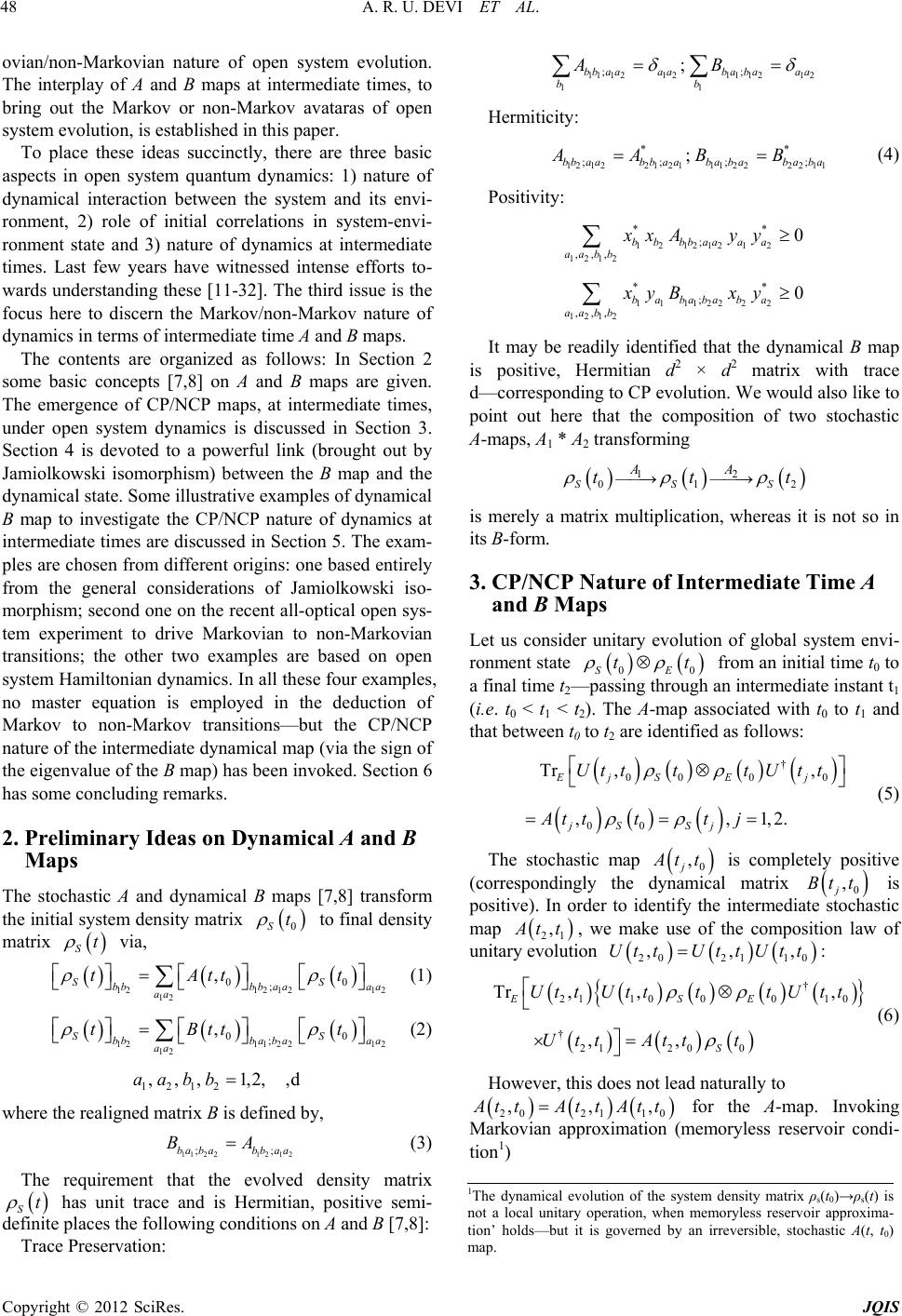

A. R. U. DEVI ET AL.
48
ovian/non-Markovian nature of open system evolution.
The interplay of A and B maps at intermediate times, to
bring out the Markov or non-Markov avataras of open
system evolution, is established in this paper.
To place these ideas succinctly, there are three basic
aspects in open system quantum dynamics: 1) nature of
dynamical interaction between the system and its envi-
ronment, 2) role of initial correlations in system-envi-
ronment state and 3) nature of dynamics at intermediate
times. Last few years have witnessed intense efforts to-
wards understanding these [11-32]. The third issue is the
focus here to discern the Markov/non-Markov nature of
dynamics in terms of intermediate time A and B maps.
The contents are organized as follows: In Section 2
some basic concepts [7,8] on A and B maps are given.
The emergence of CP/NCP maps, at intermediate times,
under open system dynamics is discussed in Section 3.
Section 4 is devoted to a powerful link (brought out by
Jamiolkowski isomorphism) between the B map and the
dynamical state. Some illustrative examples of dynamical
B map to investigate the CP/NCP nature of dynamics at
intermediate times are discussed in Section 5. The exam-
ples are chosen from different origins: one based entirely
from the general considerations of Jamiolkowski iso-
morphism; second one on the recent all-optical open sys-
tem experiment to drive Markovian to non-Markovian
transitions; the other two examples are based on open
system Hamiltonian dynamics. In all these four examples,
no master equation is employed in the deduction of
Markov to non-Markov transitions—but the CP/NCP
nature of the intermediate dynamical map (via the sign of
the eigenvalue of the B map) has been invoked. Section 6
has some concluding remarks.
2. Preliminary Ideas on Dynamical A and B
Maps
The stochastic A and dynamical B maps [7,8] transform
the initial system density matrix to final density
matrix via,

0St


St







12 12 1212
12
00
;
,
SS
bb bb aaaa
aa
tAtt t 
 

 
 (1)






12 112 212
12
00
;
,
SS
bb bab aaa
aa
tBtt t 
  
 
 (2)
1212
,,,1,2,,daabb

where the realigned matrix B is defined by,
112 2121 2
;bab abbaa
BA
;

(3)
The requirement that the evolved density matrix
has unit trace and is Hermitian, positive semi-
definite places the following conditions on A and B [7,8]:

St

Trace Preservation:
111212111212
11
;;
;
bbaa aababa aa
bb
AB

 


Hermiticity:
1212212111 222211
**
;;;
;
bbaa bbaababa baba
AABB
;
(4)
Positivity:
12 1212 12
1212
**
;
,,,
0
bbbbaaa a
aa bb
xx Ayy

1111222 2
1212
**
;
,,,
0
ba bababa
aa bb
xyBxy 

It may be readily identified that the dynamical B map
is positive, Hermitian d2 × d2 matrix with trace
d—corresponding to CP evolution. We would also like to
point out here that the composition of two stochastic
A-maps, A1 * A2 transforming

 
12
01SS
AA
tt  2S t
is merely a matrix multiplication, whereas it is not so in
its B-form.
3. CP/NCP Nature of Intermediate Time A
and B Maps
Let us consider unitary evolution of global system envi-
ronment state




0
t  0SE from an initial time t0 to
a final time t2—passing through an intermediate instant t1
(i.e. t0 < t1 < t2). The A-map associated with t0 to t1 and
that between t0 to t2 are identified as follows:
t


 




†
00 00
00
Tr,,
,,1,2
EjS Ej
jS Sj
Ut tttUt t
At tttj

 .






(5)
The stochastic map


0
,
j
A
tt is completely positive
(correspondingly the dynamical matrix


0
,
j
Bt t is
positive). In order to identify the intermediate stochastic
map


21
,
A
tt , we make use of the composition law of
unitary evolution


20
t Ut

211
,,Utt Ut

0
,t:
 


 
†
21 100010
†
2120 0
Tr ,,,
,,
ESE
S
Ut tUttttUtt
UttAttt







(6)
However, this does not lead naturally to






202110
,,,
A
ttAtt Att for the A-map. Invoking
Markovian approximation (memoryless reservoir condi-
tion1)
1The dynamical evolution of the system density matrix ρs(t0)→ρs(t) is
not a local unitary operation, when memoryless reservoir approxima-
tion’ holds—but it is governed by an irreversible, stochastic A(t, t
0)
map .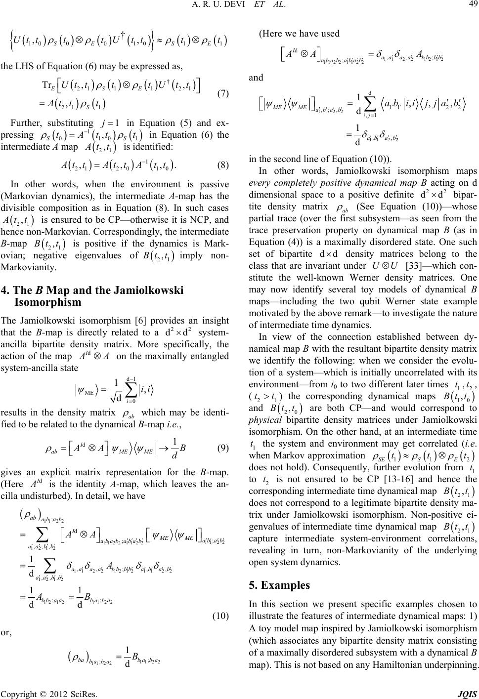

A. R. U. DEVI ET AL. 49
  

 
01110010
†
,,
SE SE
Utttt Utttt   
the LHS of Equation (6) may be expressed as,
 

†
21 1121
21 1
Tr,,
,
ESE
S
Ut tttUt t
At tt





 (7)
Further, substituting in Equation (5) and ex-
pressing 1SS in Equation (6) the
intermediate A map
1j
 
01
,tt

21
,
 
1
0
tA t 

 
A
tt is identified:






1
2120 10
,,,.
A
ttAtt Att

 (8)
In other words, when the environment is passive
(Markovian dynamics), the intermediate A-map has the
divisible composition as in Equation (8). In such cases

21
,

A
tt is ensured to be CP—otherwise it is NCP, and
hence non-Markovian. Correspondingly, the intermediate
B-map is positive if the dynamics is Mark-
ovian; negative eigenvalues ofimply non-
Markovianity.

21
,Bt t

2

21
,Bt t
4. The B Map and the Jamiolkowski
Isomorphism
The Jamiolkowski isomorphism [6] provides an insight
that the B-map is directly related to a system-
ancilla bipartite density matrix. More specifically, the
action of the map
2
dd
dI
A
A on the maximally entangled
system-ancilla state
d1
ME
0
1,
di
ii 




results in the density matrix ab

which may be identi-
fied to be related to the dynamical B-map i.e.,
d1 I
abME ME
A
A
d


 
 B (9)
gives an explicit matrix representation for the B-map.
(Here d
I
A
is the identity A-map, which leaves the an-
cilla undisturbed). In detail, we have

112 2
112 2 1122 1122
1212
112 212121122
1212
12121122
;
d
; ;
,,,
,,; ,,
,,,
;;
1
d
11
dd
ab abab
I
MEME abab
abababab
aa bb
a aaabbbba bab
aa bb
bbaabab a
AA
A
AB


 


 

 

 
 





(10)
or,

112 2
112 2;
;
1
d
bab aba
bab aB
 
(Here we have used
1 1221212
1122 1122
d
,, ;
;
I
aaa abbbb
abab abab
AA A 
 
 


 
and
11 2 2
112 22
d
112 2
,; ,
,1
,,
1,, ,
d
1
d
MEME abab
ij
abab
abiijjab 


 
 

  



in the second line of Equation (10)).
In other words, Jamiolkowski isomorphism maps
every completely positive dynamical map B acting on d
dimensional space to a positive definite 2
dd
2

bipar-
tite density matrix ab

(See Equation (10))—whose
partial trace (over the first subsystem—as seen from the
trace preservation property on dynamical map B (as in
Equation (4)) is a maximally disordered state. One such
set of bipartite dd

density matrices belong to the
class that are invariant under [33]—which con-
stitute the well-known Werner density matrices. One
may now identify several toy models of dynamical B
maps—including the two qubit Werner state example
motivated by the above remark—to investigate the nature
of intermediate time dynamics.
UU
In view of the connection established between dy-
namical map B with the resultant bipartite density matrix
we identify the following: when we consider the evolu-
tion of a system—which is initially uncorrelated with its
environment—from t0 to two different later times ,,
(2) the corresponding dynamical maps
1
t2 t
1
tt


10
t,Bt
and


20
,tBt
t
are both CP—and would correspond to
physical bipartite density matrices under Jamiolkowski
isomorphism. On the other hand, at an intermediate time
1 the system and environment may get correlated (i.e.
when Markov approximation
 



t
11SESE
does not hold). Consequently, further evolution from 1
to 2 is not ensured to be CP [13-16] and hence the
corresponding intermediate time dynamical map
2
ttt  
t


21
t,Bt
does not correspond to a legitimate bipartite density ma-
trix under Jamiolkowski isomorphism. Non-positive ei-
genvalues of intermediate time dynamical map


21
t,Bt
capture intermediate system-environment correlations,
revealing in turn, non-Markovianity of the underlying
open system dynamics.
5. Examples
In this section we present specific examples chosen to
illustrate the features of intermediate dynamical maps: 1)
A toy model map inspired by Jamiolkowski isomorphism
(which associates any bipartite density matrix consisting
of a maximally disordered subsystem with a dynamical B
map). This is not based on any Hamiltonian underpinning.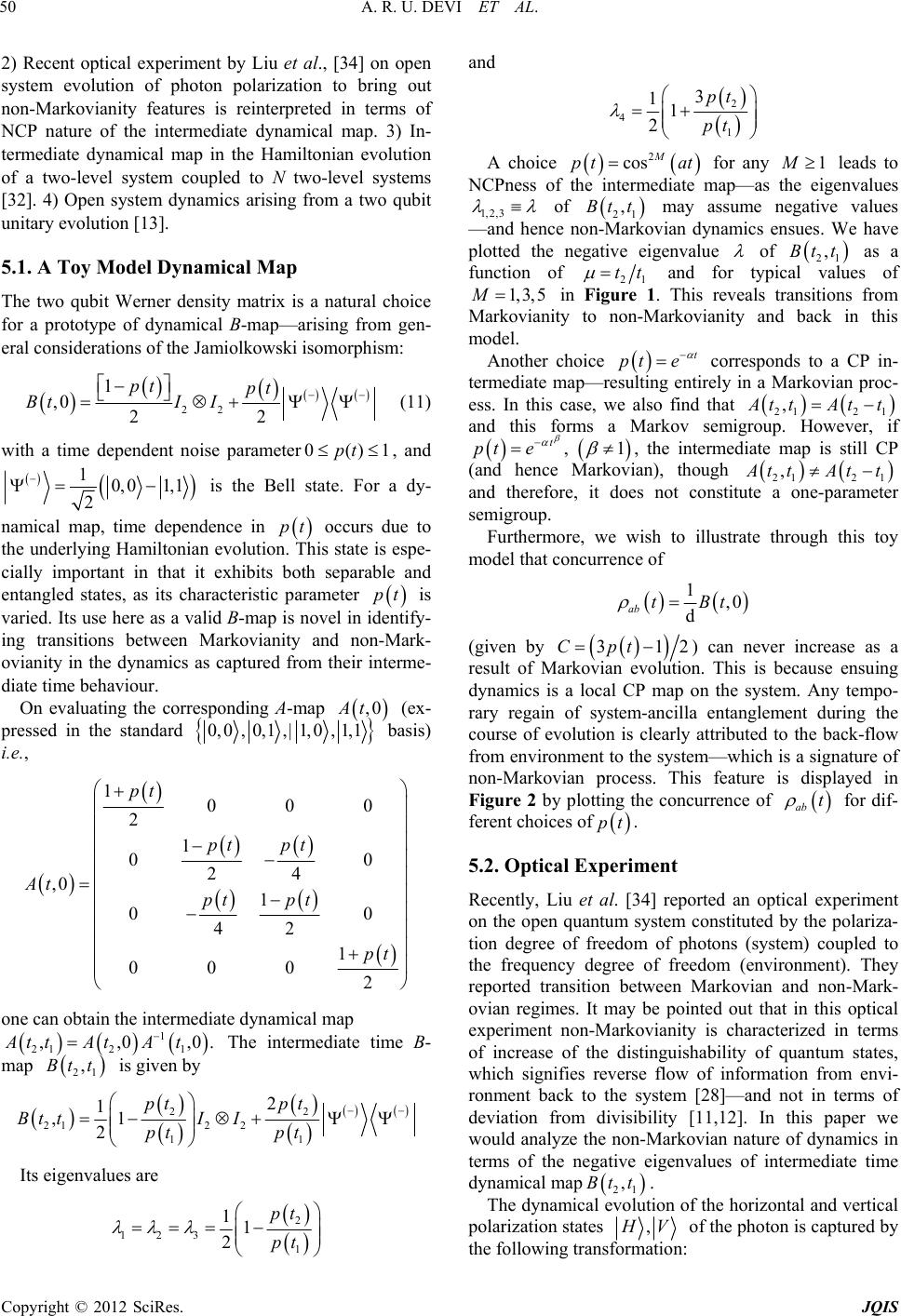

A. R. U. DEVI ET AL.
50
2) Recent optical experiment by Liu et al., [34] on open
system evolution of photon polarization to bring out
non-Markovianity features is reinterpreted in terms of
NCP nature of the intermediate dynamical map. 3) In-
termediate dynamical map in the Hamiltonian evolution
of a two-level system coupled to N two-level systems
[32]. 4) Open system dynamics arising from a two qubit
unitary evolution [13].
5.1. A Toy Model Dynamical Map
The two qubit Werner density matrix is a natural choice
for a prototype of dynamical B-map—arising from gen-
eral considerations of the Jamiolkowski isomorphism:
  
 
22
1
,0 22
pt pt
BtI I




1
(11)
with a time dependent noise parameter, and 0()pt


10, 01,1
2



is the Bell state. For a dy-
namical map, time dependence in occurs due to
the underlying Hamiltonian evolution. This state is espe-
cially important in that it exhibits both separable and
entangled states, as its characteristic parameter

pt


pt is
varied. Its use here as a valid B-map is novel in identify-
ing transitions between Markovianity and non-Mark-
ovianity in the dynamics as captured from their interme-
diate time behaviour.
On evaluating the corresponding A-map

,0

A
t (ex-
pressed in the standard

basis)
i.e.,

0, 0,0,1,|1,0,1,1


 
 

1000
2
1
0
24
,0 1
0
42
1
0002
pt
pt pt
At pt pt
pt

0
0









 





,0.


one can obtain the intermediate dynamical map
The intermediate time B-
map is given by

1
21 21
,,0At tAtAt



21
,Bt t
 



 
22
212 2
11
2
1
,1
2
pt pt
Bt tII
pt pt






Its eigenvalues are


2
123
1
11
2
pt
pt






and


2
4
1
3
11
2
pt
pt






A choice




2
cos M pt at for any 1
M
 leads to
NCPness of the intermediate map—as the eigenvalues
1, 2, 3



of


21
,Bt t may assume negative values
—and hence non-Markovian dynamics ensues. We have
plotted the negative eigenvalue

of 21 as a
function of

,Bt

t
21
tt


and for typical values of
1, 3, 5M

in Figure 1. This reveals transitions from
Markovianity to non-Markovianity and back in this
model.
Another choice


t
pte


 corresponds to a CP in-
termediate map—resulting entirely in a Markovian proc-
ess. In this case, we also find that



212 1
,
A
ttAt t


and this forms a Markov semigroup. However, if
 
,
t
pte





1

, the intermediate map is still CP
(and hence Markovian), though



2121
,
A
ttAtt
and therefore, it does not constitute a one-parameter
semigroup.
Furthermore, we wish to illustrate through this toy
model that concurrence of
 
1,0
d
ab tBt
 
(given by




31Cpt2) can never increase as a
result of Markovian evolution. This is because ensuing
dynamics is a local CP map on the system. Any tempo-
rary regain of system-ancilla entanglement during the
course of evolution is clearly attributed to the back-flow
from environment to the system—which is a signature of
non-Markovian process. This feature is displayed in
Figure 2 by plotting the concurrence of


ab t
 for dif-
ferent choices of


pt.
5.2. Optical Experiment
Recently, Liu et al. [34] reported an optical experiment
on the open quantum system constituted by the polariza-
tion degree of freedom of photons (system) coupled to
the frequency degree of freedom (environment). They
reported transition between Markovian and non-Mark-
ovian regimes. It may be pointed out that in this optical
experiment non-Markovianity is characterized in terms
of increase of the distinguishability of quantum states,
which signifies reverse flow of information from envi-
ronment back to the system [28]—and not in terms of
deviation from divisibility [11,12]. In this paper we
would analyze the non-Markovian nature of dynamics in
terms of the negative eigenvalues of intermediate time
dynamical map


21
,Bt t.
The dynamical evolution of the horizontal and vertical
polarization states ,
H
V of the photon is captured by
the following transformation:

A. R. U. DEVI ET AL. 51
Figure 1. A plot of the eigenvalue

of versus (,)
21
Bt t
μ=tt
21
for different values of M. The dynamics is non-
Markovian when

assumes negative values and other-
wise it is Markovian.
Figure 2. Concurrence




31C=p t2 of the system-
ancilla state
 


22



1
4
abME ME
pt
ρt=I I+ptψψ,
vs. scaled time at, for the following choices i) Markov proc-
ess:


at
pt =e
 
cos2M
(solid line) and ii) non-Markov process:

1
p
t=at,M= (dashed line) and (dot-
dashed line). Note that there is a death and re-birth of en-
tanglement (dash, dot-dashed lines) due to back-flow from
environment.
M=5
H
HHH
VV VV


*
H
VtH  V


VH tVH 
Here denotes the decoherence function, mag-
nitude of which is modelled as,

t 





2
2
2
2
1
22
1
2
2
11
12
1
·
141s
cos
in 2
nt
nt
nt
e
tAA
A
nt
eAA



















(14)
where VH nn n


2
is the difference between the re-
fractive indices of vertically and horizontally polarized
light; 1



 distance between two frequency
peaks (for details see [34]), 11
1,0 1.
1
AA
A



The corresponding A and B maps (in the


,,,
H
HHVVHVV basis) are readily identified to be,
  
*
10 00
00
,0 000
00 01
t
At t








0



*
100
000 0
,0 000 0
00 1
t
Bt
t









We construct the intermediate time dynamical map


21
,Bt tfrom the corresponding






1
21 21
,,0AtAt

Att,0 to obtain,





*
2
*
1
21
2
1
100
000 0
,.
000 0
00 1
t
t
Bt t
t
t














(16)
Eigenvalues of


21
,Bt t are given by,



2
1,4 2,3
1
1,
t
t



0.


 (17)
The eigenvalue 4

can assume negative values indi-
cating Markovian/non-Markovian regimes. A plot of the
negative eigenvalue as a function of 1
A
, for different
ratios 21 tt (for the choice of parameters
Hz, Hz, which are em-
ployed in Ref. [34]) is given in Figure 3 where one can
clearly see the Markovian (
13
1.6 10   12 1.8 10
40


) and non-Markovian
(40


) regimes.
5.3. Hamiltonian Evolution of a Two Level
System Coupled to a Bath of N Spins
We now present a Hamiltonian model, which give rise to
explicit structure of time dependence in the open system
evolution. Interaction Hamiltonian considered here is
[28,32]
1
.
N
z
kz
k
A
HN



 (18)

A. R. U. DEVI ET AL.
52
Figure 3. A plot of the eigenvalue of λ4


,
21
Bt t versus
for different values of
A1μ=t t
1
=1.
2 and for the choice of
parameters Hz, Hz. 13 Δ=1.610ω 12 108σ
This is a simplified model of a hyperfine interaction of a
spin—1/2 system with N spin—1/2 nuclear environ-
ment in a quantum dot. Taking the initial system-envi-
ronment state to be

2
02
N
S
N
I
 , the dynamical A-map
is obtained by evaluating
 
† 2
Tr,0 0,0
2
N
ES
N
I
UtU t






(where
 

,0 ExpUt iHt):
 




22
11
,0 11,
22
2
cos.
zz
N
A
txt xtI
At
xt N
  



I

(19)
From this, the intermediate map

21
,
A
tt

,Bt
(see Equa-
tion (8)) and in turn the corresponding may be
readily evaluated. We obtain,

21
t




2122
2
1
1
,2
.
2
zz
xxyy
Bt tII
xt
xt






(20)
The eigenvalues of are

21
,Bt t



2
1
0, 0,1.
x
t
x
t

Clearly, the intermediate time dynamics exhibits NCP
nature as one of the eigenvalues i.e.



2
1
1
x
t
x
t
  of

21
,Bt t

can assume negative values.
We illustrate regimes of Markovianity/non-Markovi-
anity revealed via positive/negative values of

(plot
ted as a function of 21
tt

) in Figure 4.
Figure 4. The variation of the eigenvalue
λ
of


,
21
Bt t
(as a function of μ=t t
21
) from positive to negative values
and back with the passage of time for different values of N.
5.4. Two Qubit Unitary Evolution
We now consider the open system dynamics arising from
the unitary evolution [13]

 
22
,0
cos 2 sin2
zx
it
z
x
Ut e
tIIi t
 


 


 
(21)
on the system-environment initial state
   
22
11
000
22
SE SExz
II    .
The (,0)
A
t map is given by,
 

 
22
1
,01cos
2
11cos.
2
z
z
Att II
t



 
 
(22)
Following Equation (8), we obtain




2122
2
1
1
,2
cos
.
2cos
zz
xxy y
Bt tII
t
t





(23)
The eigenvalues of the B-map are given by
2
1
cos
0, 0,1cos
t
t


. The eigenvalue 2
1
cos
1cos
t
t



 can
assume negative values—bringing out the non-Mark-
ovian features prevalent in the dynamical process. Fig-
ure 5 illustrates the transitions from Markovianity to
non-Markovianity. This model, with initially correlated
states, has been explored before in Refs. [13,17] and the
dynamical map turned out to be NCP throughout not
merely in the intermediate time interval).
6. Summary
In conclusion, a few remarks on a variety of definitions

A. R. U. DEVI ET AL. 53
Figure 5. The plot of the eigenvalue cos
cos
2
1
1ωt
λ=ωt
 as a
function of μ=tt
21
. The periodic transitions of
λ
from
positive to negative values indicates the transition of the
process from Markovian to non-Markovian.
of non-Markovianity in the recent literature may be re-
called here. Mainly the focus has been towards capturing
the violation of semi-group property [17,27] or more
recently—its two-parameter generalization viz the divisi-
bility of the dynamical map [11,12]. Yet another measure,
where non-Markovianity [28] is attributed to increase of
distinguishability of any pairs of states (as a result of the
partial back-flow of information from the environment
into the system) and is quantified in terms of trace dis-
tance of the states. It has been shown that the two differ-
ent measures of non-Markovianity—one based on the
divisibility of the dynamical map [12] and the other
based upon the distinguishability of quantum states [28]
—need not agree with each other [29,30]. A modified
version of the criterion of Ref. [12] was proposed re-
cently [32]. In this paper we have established the inter-
play of stochastic A and dynamical B maps at intermedi-
ate times, revealing Markovian/non-Markovian regimes.
We have explored four different examples revealing the
features of intermediate time maps originating from vari-
ety of physical mechanisms: 1) A toy model map in-
spired by general considerations based on Jamiolkowski
isomorphism—which explores a two qubit Werner state
with time-dependent noise parameter as a dynamical map;
2) A reinterpretation of the phenomenological model
explaining the recent optical experiment by Liu et al., [34]
in terms of NCP nature of the intermediate B map; 3)
Hamiltonian evolution describing the hyperfine interact-
tion of a spin—1/2 system with N spin—1/2 nuclear en-
vironment in a quantum dot [32] displaying Mark-
ovian/non-Markovian behavior and 4) Unitary evolution
of Jordan et al., [13]—wherein initial system-environ-
ment two qubit is chosen in a product state. Here too,
intermediate time dynamical map exhibits Markov/non-
Markov regimes. It is interesting to note that the dy-
namics had been identified to be NCP throughout not
merely in the intermediate time interval—when initially
correlated states were employed [13,17]. Placing these
two results together, brings forth that the source of non-
Markovianity in this model is attributable entirely to the
unitary dynamics—rather than initial correlations of sys-
tem-environment qubits. We have thus exposed the un-
derlying features of intermediate time A and B maps to
bring out clearly if the dynamics relies on past history of
the states or not.
REFERENCES
[1] H. P. Breuer and F. Petruccione, “The Theory of Open
Quantum Systems,” Oxford University Press, Oxford,
2007. doi:10.1093/acprof:oso/9780199213900.001.0001
[2] R. Alicki and K. Lendi, “Quantum Dynamical Semi-
Groups and Applications,” Springer, Berlin, 1987.
[3] M. A. Nielsen and I. L. Chuang, “Quantum Computation
and Quantum Information,” Cambridge University Press,
Cambridge, 2000.
[4] M. D. Choi, “Positive Linear Maps on C*-Algebras,”
Canadian Journal of Mathematics, Vol. 24, No. 3, 1972,
pp. 520-529.
[5] M. D. Choi, “Completely Positive Linear Maps on Com-
plex Matrices,” Linear Algebra and Its Applications, Vol.
10, No. 3, 1975, pp. 285-290.
doi:10.1016/0024-3795(75)90075-0
[6] A. Jamiolkowski, “Linear Transformations Which Pre-
serve Trace and Positive Semidefiniteness of Operators,”
Reports on Mathematical Physics, Vol. 3, No. 4, 1972, pp.
275-278. doi:10.1016/0034-4877(72)90011-0
[7] E. C. G. Sudarshan, P. Mathews and J. Rau, “Stochastic-
Dynamics of Quantum-Mechanical Systems,” Physical
Review, Vol. 121, No. 3, 1961, pp. 920-924.
[8] T. F. Jordan and E. C. G. Sudarshan, “Dynamical Map-
Pings of Density Operators in Quantum Mechanics,”
Journal of Mathematical Physics, Vol. 2, No. 6, 1961, pp.
772-775.
[9] G. Lindblad, “On the Generators of Quantum Dynamical
Semigroups,” Communications in Mathematical Physics,
Vol. 48, No. 2, 1976, pp. 119-130.
doi:10.1007/BF01608499
[10] V. Gorini, A. Kossakowski and E. C. G. Sudarshan,
“Completely Positive Dynamical Semigroups of N-Level
Systems,” Journal of Mathematical Physics, Vol. 17, No.
5, 1976, pp. 821-825. doi:10.1063/1.522979
[11] M. M. Wolf, J. Eisert, T. S. Cubitt and J. I. Cirac, “As-
sessing Non-Markovian Quantum Dynamics,” Physical
Review Letters, Vol. 101, No. 15, 2008, pp. 150402.1-
150402.4.
[12] A. Rivas, S. F. Huelga and M. B. Plenio, “Entanglement
and Non-Markovianity of Quantum Evolutions,” Physical
Review Letters, Vol. 105, No. 5, 2010, pp. 050403.1-
050403.4.
[13] T. F. Jordan, A. Shaji and E. C. G. Sudarshan, “Dynamics
of Initially Entangled Open Quantum Systems,” Physical

A. R. U. DEVI ET AL.
54
Review A, Vol. 70, No. 5, 2004, pp. 052110.1-052110.14.
[14] C. A. Rodríguez-Rosario and E. C. G. Sudarshan, “Non-
Markovian Open Quantum Systems,” Bulletin of the
American Physical Society, Vol. 53, No. 2, 2008.
[15] C. A. Rodríguez-Rosario, K. Modi, A. Kuah, A. Shaji and
E. C. G. Sudarshan, “Completely Positive Maps and
Classical Correlations,” Journal of Physics A, Vol. 41, No.
20, 2008, pp. 205301.1-205301.8.
[16] K. Modi and E. C. G. Sudarshan, “Role of Preparation in
Quantum Process Tomography,” Physical Review A, Vol.
81, No. 5, 2010, pp. 052119.1-052119.10.
[17] A. R. Usha Devi, A. K. Rajagopal and Sudha, “Open-
System Quantum Dynamics with Correlated Initial States,
Not Completely Positive Maps, and Non-Markovianity,”
Physical Review A, Vol. 83, No. 2, 2011, pp. 022109.1-
022109.8.
[18] H.-P. Breuer, “Exact Quantum Jump Approach to Open
Systems in Bosonic and Spin Baths,” Physical Review A,
Vol. 69, No. 2, 2004, pp. 022115.1-022115.8.
[19] H. P. Breuer, “Genuine Quantum Trajectories for Non-
Markovian Processes,” Physical Review A, Vol. 70, No. 1,
2004, pp. 012106.1-012106.12.
[20] S. Daffer, K. Wódkiewicz, J. D. Cresser and K. McIver,
“Depolarizing Channel as a Completely Positive Map
with Memory,” Physical Review A, Vol. 70, No. 1, 2004,
pp. 010304.1-010304.4.
[21] H.-P. Breuer and B. Vacchini, “Quantum Semi-Markov
Processes,” Physical Review Letters, Vol. 101, No. 14,
2008, pp. 140402.1-140402.4.
[22] H.-P. Breuer and B. Vacchini, “Structure of Completely
Positive Quantum Master Equations with Memory Ker-
nel,” Physical Review E, Vol. 79, No. 4, 2009, pp.
041147.1-041147.12.
[23] A. Kossakowski and R. Rebolledo, “On Non-Markovian
Time Evolution in Open Quantum Systems,” Open Sys-
tems and Information Dynamics, Vol. 14, No. 3, 2007, pp.
265-274. doi:10.1007/s11080-007-9051-5
[24] A. Kossakowski and R. Rebolledo, “On Completely Posi-
tive Non-Markovian Evolution of a d-Level System,”
Open Systems and Information Dynamics, Vol. 15, No. 2,
2008, pp. 135-141.
[25] A. Kossakowski and R. Rebolledo, “On the Structure of
Generators for Non-Markovian Master Equations,” Open
Systems and Information Dynamics, Vol. 16, No. 2-3,
2009, pp. 259-268.
[26] D. Chruściński and A. Kossakowski, “Non-Markovian
Quantum Dynamics: Local versus Nonlocal,” Physical
Review Letters, Vol. 104, No. 7, 2010, pp. 070406.1-
070406.4.
[27] A. K. Rajagopal, A. R. Usha Devi and R. W. Rendell,
“Kraus Representation of Quantum Evolution and Fidel-
ity as Manifestations of Markovian and Non-Markovian
Forms,” Physical Review A, Vol. 82, No. 4, 2010, pp.
042107.1-042107.7.
[28] H.-P. Breuer, E. M. Laine and J. Piilo, “Measure for the
Degree of Non-Markovian Behavior of Quantum Proc-
esses in Open Systems,” Physical Review Letters, Vol.
103, No. 21, 2009, pp. 210401.1-210401.4.
[29] E. M. Laine, J. Piilo and H.-P. Breuer, “Measure for the
Non-Markovianity of Quantum Processes,” Physical Re-
view A, Vol. 81, No. 6, 2010, pp. 062115.1-062115.8.
[30] P. Haikka, J. D. Cresser and S. Maniscalco, “Comparing
Different Non-Markovianity Measures in a Driven Qubit
System,” Physical Review A, Vol. 83, No. 1, 2011, pp.
012112.1-012112.5.
[31] D. Chruściński, A. Kossakowski and A. Rivas, “Measures
of Non-Markovianity: Divisibility versus Backflow of
Information,” Physical Review A, Vol. 83, No. 5, 2011,
pp. 052128.1-052128.6.
[32] S. C. Hou, X. X. Yi, S. X. Yu and C. H. Oh, “Alternative
Non-Markovianity Measure by Divisibility of Dynamical
Maps,” Physical Review A, Vol. 83, No. 6, 2011, pp.
062115.1-062115.6
[33] K. G. H. Vollbrecht and R. F. Werner, “Entanglement
Measures under Symmetry,” Physical Review A, Vol. 64,
No. 6, 2001, pp. 062307.1-062307.15
[34] B.-L. Liu, L. Li, Y.-F. Huang, C.-F. Li, G.-C. Guo, E.-M
Laine, H.-P. Breuer and J. Piilo, “Experimental Control of
the Transition from Markovian to Non-Markovian Dy-
namics of Open Quantum Systems,” Nature Physics, Vol.
7, No. 12, 2011, pp. 931-934. doi:10.1038/nphys2085
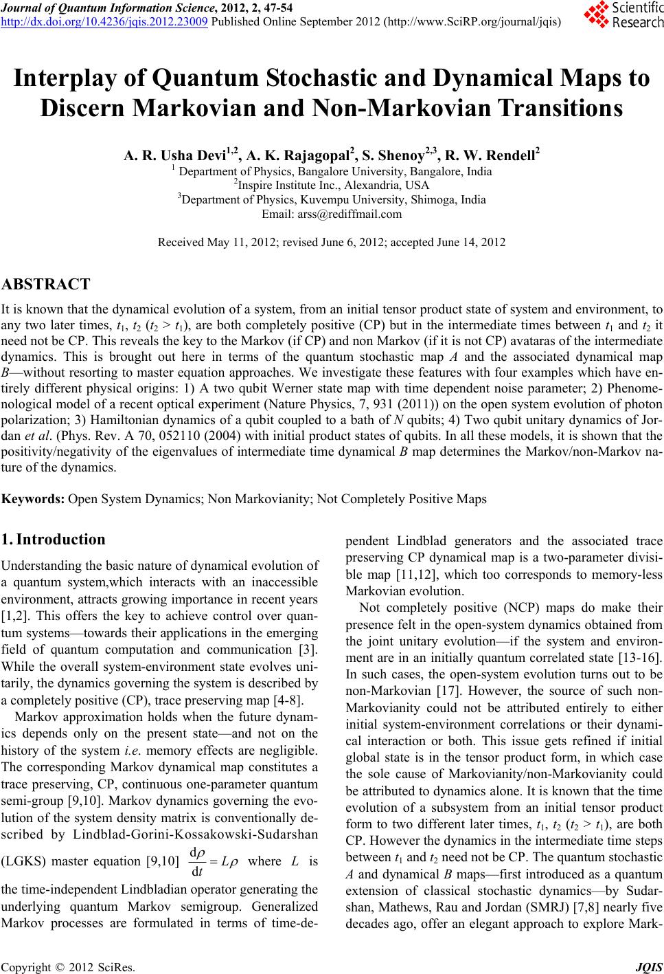