ABSTRACT

In this paper we consider three problems in continuous multi-criteria optimization: An application of the Berge Maximum Theorem, properties of Pareto-retract mappings, and the structure of Pareto sets. The key goal of this work is to present the relationship between the three problems mentioned above. First, applying the Maximum Theorem we construct the Pareto-retract mappings from the feasible domain onto the Pareto-optimal solutions set if the feasible domain is compact. Next, using these mappings we analyze the structure of the Pareto sets. Some basic topological properties of the Pareto solutions sets in the general case and in the convex case are also discussed.

1. Introduction

The Berge Maximum Theorem, shortly the Maximum Theorem, has become one of the most useful and powerful theorems in optimization theory, mathematical economics and game theory. The original variant of the Maximum Theorem is as follows:

Theorem 1 [1] [2, Theorem 9.14]. Let and, be a continuous function, and be a compact-valued and continuous multifunction. Then, the function defined by is continuous on X, and the multifunction defined by is compact-valued and upper semi-continuous on X.

The Maximum Theorem is often used in a special situation when the multifunction D is convex-valued and the function u is quasi-concave or concave in its second variable in addition to the hypotheses of Theorem 1.

Now, we give a presentation of the classical variant of the Maximum Theorem.

Theorem 2 [2, Theorem 9.17 and Corollary 9.20]. Let and, be a continuous function, and be a compact-valued and continuous multifunction. Define m and S as in Theorem 1.

(a) Then m is a continuous function on X, and S is a compact-valued and upper semi-continuous multifunction on X.

(b) If is quasi-concave in y for each, and D is convex-valued, then S is convex-valued.

(c) If is strictly quasi-concave in y for each, and D is convex-valued, then S is a continuous function on X.

(d) If u is concave on, and D has a convex graph, then m is a concave function on X and S is a convex-valued multifunction on X.

(e) If u is strictly concave on, and D has a convex graph, then m is a strictly concave and continuous function on X, and S is a continuous function on X.

Remark 1. It is important to note the following two facts [2, Example 9.15 and 9.16]:

(1) S is only upper semi-continuous, and not necessarily also lower semi-continuous.

(2) The continuity of u on cannot be replaced with one of separate continuity, i.e., that is continuous on X for each fixed and that is continuous on Y for each fixed.

Let us consider Theorem 2. It is possible to have for all. Obviously, the following theorem is true.

Theorem 3. Let and, be a continuous function, and be a compact-valued and continuous multifunction. Define m and S as in Theorem 1. If for all, then m and S are two continuous function on X.

2. Basic Concepts and Definitions

It is easy to show that Theorems 1, 2 and 3 imply the following two theorems.

Theorem 4. Let, be a continuous function, and be a continuous multifunction. Then, the function defined by is continuous on X, and the multifunction defined by 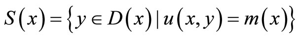is upper semi-continuous on X.

Theorem 5. Let, be a continuous function, and be a continuous multifunction. Define m and S as in Theorem 4. If for all, then m and S are two continuous function on X.

Now we will apply these two theorems to multi-criteria optimization.

The general form of the multi-criteria unconstrained optimization problem is to find a variable , , so as to maximize subject to, where the feasible domain X is nonempty and compact, is the index set, , is a given objective continuous function for all.

Now we will introduce several solution concepts for our multi-criteria optimization problem.

Definition 1.

(a) A point is called an ideal Pareto-optimal solution if and only if for all and all. The set of the ideal Pareto-optimal solutions of X is denoted by and is called an ideal Pareto-optimal set.

(b) A point is called a Pareto-optimal solution if and only if there does not exist a point such that for all and for some. The set of the Pareto-optimal solutions of X is denoted by and is called a Pareto-optimal set. Its image is called a Pareto-front set.

(c) A point is called a strictly Pareto-optimal solution if and only if there does not exist a point such that for all and. The set of the strictly Pareto-optimal solutions of X is denoted by and is called a strictly Pareto-optimal set.

The above definition qualifies Pareto-optimal solutions in the global sense.

In literature, the term Pareto-optimal is frequently used synonymously with efficient, non-inferior and non-dominated.

In our optimization problem, it can be shown that: is nonempty, but and may be empty; and , see also [3-5].

Remark 2. It is well-known that when is nonempty [6].

Usually, a Pareto-optimal solution is not necessarily uniquely determined, but there are several Pareto-optimal solutions.

For a better understanding of this paper, we recall some useful notations and definitions.

To be precise, we introduce the following notations: for every two vectors, means for all, means for all (weakly component-wise order), means for all (strictly component-wise order), and means for all and for some (component-wise order).

Remark 3. Let X and Y be two topological spaces. A homotopy between two continuous functions is defined to be a continuous function such that and for all. Note that we can consider the homotopy H as a continuously deformation of f to g [7].

Definition 2.

(a) The set is a retract of X if and only if there exists a continuous function such that for all. The function r is called a retraction of X to Y.

(b) The set is a deformation retract of X if and only if there exist a retraction and a homotopy 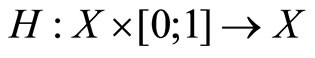such that and 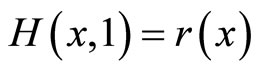for all.

Remark 4. From a more formal viewpoint, a retraction is a function such that 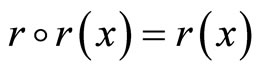for all, since this equation says exactly that r is the identity on its image. Retractions are the topological analogs of projection operators in other parts of mathematics. It is true that every deformation retract is a retract, but in generally the converse does not hold [7].

Applications of retractions in multi-criteria optimization have been discussed by several authors [3,8-12].

We are now ready to define:

1) A multifunction by 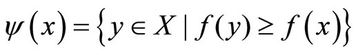for all.

2) A multifunction by 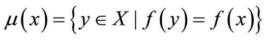for all.

3) A function by for all.

Note that, for each, is equal to the intersection of all the upper contour sets and is equal to the intersection of all the level sets. Clearly, for all.

Remark 5. From Definition 1 it is easy directly verify that for:

(1) is equivalent to (or equivalently).

(2) is equivalent to.

Choose and consider an optimization problem with a single objective function as follows: 1) Maximize subject to or 2) maximize subject to. By letting x vary over all of X we can identify different Pareto-optimal solutions. This optimization technique will allow us to find the whole Paretooptimal set and analyze its structure.

Remark 6. It is known that for all [6].

The above remark allows us to present a new definition.

Definition 3.

(a) A multifunction is a called Pareto-retract (Pareto-retract point-to-set mapping) if and only if for all.

(b) A function is called a Paretoretract (Pareto-retract point-to-point mapping) if and only if for all.

Thus we introduce the concept of the Pareto-retract mappings. Here the fundamental idea is based on the observation that for any which is not Paretooptimal there exists at least one other such that for all and strictly inequality holds at least once.

According to Remark 6, one can see that there exists a Pareto-retract multifunction, but an open problem is its continuity (lower or upper semi-continuous).

3. Assumptions and Theorems in the General Case

In this section, we will discuss the role of the following assumptions that affect the characteristics of a Paretoretract mapping (Pareto-retract multifunction and Paretoretract function) if the feasible domain X is compact:

Assumption 1. is lower semi-continuous on X.

Assumption 2a. for all.

Assumption 2b. There exists such that for all.

Note that if Assumption 2a holds, then there exists a Pareto-retract function, see also Remark 6. Again, an open problem is its continuity.

These assumptions allow us to present our theorems of this section.

Theorem 6. is upper semi-continuous on X.

Proof. We will prove that if and are a pair of sequences such that and for all, then there exists a convergent subsequence of whose limit belongs to.

The assumption for all implies for all. From the condition it follows that there exists a convergent subsequence such that . Therefore, there exists a convergent subsequence such that and. Thus, we find that for all. Taking the limit as we obtain, i.e.. This means that is upper semi-continuous on X.

The theorem is proven.

We are now ready to prove the following basic theorem.

Theorem 7. If Assumption 1 holds, then:

(a) is continuous on X.

(b) There exists an upper semi-continuous Pareto-retract multifunction.

(c) and are compact.

Proof.

(a) Assumption 1 and Theorem 6 imply that is continuous on X.

(b) According Remark 6 we are in a position to construct a multifunction such that for all. It is easy to show that for. This means that.

The function s is continuous and the multifunction is compact-valued and continuous. Now applying Theorem 4, we conclude that is an upper semi-continuous multifunction on the compact domain X.

(c) We recall that X is compact; therefore, part (b) implies that is compact too. Trivially, is compact.

The theorem is proven.

Remark 7. Let Assumption 1 be satisfied. Remark 1 shows that the multifunction is not necessarily lower semi-continuous.

Theorem 8. If Assumption 2a or 2b holds, then.

Proof. It is well-known that.

Let and assume that. From the fact that it follows that there exists such that for all and. Hence,.

There are two cases:

(1) If Assumption 2a holds, then there exists a unique such that for all. But we get that and. This means that, and for all. As a result we obtain for all and for some. This leads to a contradiction.

(2) If Assumption 2b holds, then there exists a unique such that for all. But we know that for all and. This means that, for all and. This leads to a contradiction too.

Finally, we obtain.

The theorem is proven.

Remark 8. While studying the proof of Theorem 8, one can see that if and, then.

Theorem 9. If Assumptions 1 and 2a (or 1 and 2b) hold, then:

(a) There exists a continuous Pareto-retract function.

(b) is homeomorphic to.

Proof. (a) First, let Assumptions 1 and 2a be satisfied. In this case, we construct a function such that for all. From Theorems 5, 7 and 8, and Remark 6 it follows that r is a continuous Pareto-retract function.

For the second part of this proof, let Assumptions 1 and 2b be satisfied. Now we construct a function such that for all. From Theorems 5, 7 and 8, and Remark 8 it follows that r is a continuous Pareto-retract function.

(b) Recalling that the function is continuous; therefore, a restriction of f is continuous too. From Remark 5 and Theorem 8 we have that the function h is bijective. Consider the inverse function of h. We proved in Theorem 7 that is compact; therefore, is continuous too [13]. As a result we conclude that the function h is homeomorphism.

The theorem is proven.

Remark 9. From Theorem 9 we can easily check the following:

(1) For each, is nonempty compact and.

(2) If and, then .

(3).

(4) By Assumption 2a, for each we have and for all .

(5) By Assumption 2b, for each we have and for all .

4. Structure of Pareto Sets

The structure of Pareto sets is very important, from an algorithmic point of view.

Let be the Euclidean metric in and be the topology induced by. In a topological space, for we now recall some general topological definitions.

Definition 4. A property is called a topological property if and only if an arbitrary topological space X has this property, then Y has this property too, where Y is homeomorphic to X.

Definition 5.

(a) The set Y is connected if and only if it is not the union of a pair of nonempty sets of, which are disjoint.

(b) The set Y is path-wise connected if and only if for every there exists a continuous function such that and. The function p is called a path.

(c) The set Y is simply connected if and only if it is path-wise connected and every path between two points can be continuously deformed into every other.

(d) The set Y is contractible (contractible to a point) if and only if there exists a point such that is a deformation retract of Y.

Remark 10. Recalling that the following statements are true:

(1) Convexity implies contractibility, contractibility implies simply connectedness, simply connectedness implies path-wise connectedness, and path-wise connectedness implies connectedness. However, in general the converse does not hold.

(2) Contractibility, simply connectedness, path-wise connectedness and connectedness are topological properties of sets.

(3) Compactness, path-wise connectedness and connectedness of sets are preserved under a continuous function.

(4) Compactness, connectedness, path-wise connectedness, simply connectedness and contractibility of sets are preserved a under retraction.

(5) The image of a simply connected set under a continuous function need not to be simply connected.

(6) The image of a convex set under a retraction need not to be convex.

Remark 11. We now focus our attention to contractibility of sets. Let. Remark 10 has shown that if Y is a retract of X and X is contractible, then Y is contractible too. The converse does not hold in generally. But for every deformation retract the following statement is true: “If Y is a deformation retract of X, then Y is contractible if and only if X is contractible.”

Definition 6.

(a) The topological space Y is said to have the fixed point property if and only if every continuous function from this set into itself has a fixed point, i.e. there is a point such that.

(b) The topological space Y is said to have the Kakutani fixed point property if and only if every upper semi-continuous multifunction from this set into itself has a fixed point, i.e. there is a point such that.

(1) Remark 12. We will use the following statements for each compact set:

Convexity implies the fixed point properties (fixed point property and Kakutani fixed point property).

(2) The fixed point properties of sets are topological properties.

(3) The fixed point properties of sets are preserved under retraction.

(4) A set having the fixed point property is equivalent to this set having the Kakutani fixed point property.

Now we focus our attention on the compactness, connectedness, contractibility and fixed point properties of the Pareto sets. Compactness of these sets is studied in [3,8,12,14-16]. Connectedness is considered in [3,6,8, 16-24]. Contractibility of Pareto sets is discussed in [9, 10,12,25]. Fixed point properties have been addressed in [10,12,26].

Corollary 1. If Assumptions 1 and 2a (or 1 and 2b) hold, then:

(a) If X is convex, then and are contractible and have the fixed point properties.

(b) If X is contractible, then and are contractible.

(c) If X is simply connected, then and are simply connected.

(d) If X is path-wise connected, then and are path-wise connected.

(e) If X is connected, then and are connected.

(f) If X has the fixed point properties, then and have the fixed point properties.

Proof. Directly, from Theorem 9, Remarks 10 and 12 imply the proof.

5. Convex Case

We often use the Maximum Theorem under convexity as a mathematical tool in convex optimization. Here we will present two special variants of this theorem and their applications to convex multi-criteria optimization.

In this section, we are going to study our optimization problem when the functions are concave and a function of is strictly quasi-concave on the compact and convex domain X.

Concavities of the objective functions play a central role in optimization theory, for more information see [27] and [28]. We will use the definitions of quasi-concave and concave functions in the usual sense.

Definition 7. A real function g on a convex subset is called to be:

(a) Quasi-concave on X if and only if for any and, then .

(b) Strictly quasi-concave on X if and only if for any, and, then .

(c) Concave on X if and only if for any and, then.

Now, from Theorems 2 and 4 we get the first special variant of the Maximum Theorem under convexity.

Theorem 10. Let, be a continuous function, and be a continuous multifunction. Define m and S as in Theorem 4. If u is quasiconcave on X and D is convex-valued, then S is a convex-valued and upper semi-continuous multifunction on X.

Remark 13. If are all quasi-concave and one of them is strictly quasi-concave, then [3,6].

We are ready to prove the first theorem in this section.

Theorem 11. Let be all concave on the compact and convex domain X. Then:

(a) is convex-valued and continuous on X. In particular, Assumption 1 holds.

(b) There exists an upper semi-continuous Pareto-retract multifunction.

(c) and are compact.

(d) is convex when.

(e) for all .

(f) There exists a continuous function such that. In particular, is path-wise connected.

Proof. (a) Define a multifunction such that 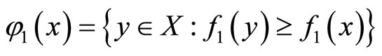for all. It is easy to show that the multifunction is convex-valued.

We will prove continuity of on X using a two-step procedure.

Step 1. We will prove that if and are a pair of sequences such that and for all, then there exists a convergent subsequence of whose limit belongs to.

The assumption for all implies for all. From the condition it follows that there exists a convergent subsequence such that. Therefore, there exists a convergent subsequence such that and . Thus, we find that for all. Taking the limit as we obtain . As a result we have. In other words, is upper semi-continuous on X.

Step 2. We will prove that if is a sequence convergent to and, then there exists a sequence such that for all and.

There are two cases:

(1) Suppose that.

We get that, i.e.. In this case let.

(2) Suppose that.

In this case, we will consider two possibilities:

(2.1) Suppose that.

From implies. Without loss of generally we can study the case when . As a result we obtain and let.

(2.2) Suppose that.

From the fact that is continuous and concave on the compact and convex domain X, we deduce that is nonempty, convex and compact. Denote the distance between and by. Clearly, and there exists a unique such that. Consider a linear segment and a restriction of. From the definition of b it follows that: 1) If and, then, 2) if and, then for all, i.e. implies. It is easy to show that b is bijective and continuous on; therefore, there exists a unique such that and is continuous. We obtain:, , , ,.

As a result we get a sequence such that for all and. This means that is lower semi-continuous on X.

In summary, is continuous on X.

Now, define a multifunction such that 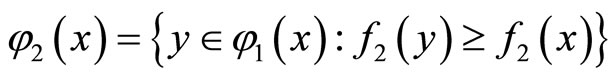for all. By analogy, we prove that is convex-valued and continuous on X.

This procedure is repeated until all objective functions have been considered. At the end, define a multifunction such that 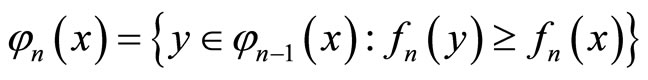for all. Similarly, we prove that is convex-valued and continuous on X.

Observe that. Hence, is continuous on X and Assumption 1 holds.

(b) The proof follows directly from Theorems 7(b) and 11(a).

(c) This is immediate from Theorems 7(c) and 11(a).

(d) If is nonempty, then . In fact is nonempty and convex, we deduce that is convex.

(e) It is obvious that for all.

We will prove that if, then.

There are two possibilities:

(1) Suppose that.

The statement is trivially true.

(2) Suppose that.

Let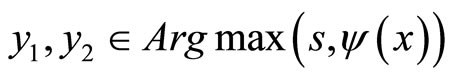, , and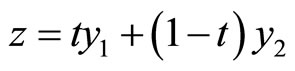. In fact, is convex, it follows that 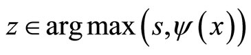and s (z) = s (y₁) = s (y₂). But for each there is. By using this result we derive that. Since implies. This means that for all and all, i.e. for all. Thus, we get for all, i.e..

Finally, according to this result and Remarks 5 and 6 we conclude that for all.

(f) Consider the multifunction from Theorem 7(b). Theorem 11(e) allows us to define a function by. The function b is continuous on X because ρ is upper semicontinuous on X and f is continuous on. Clearly,.

So, we get the continuous function b and we know that X is path-wise connected; therefore, is pathwise connected too.

The theorem is proven.

Note that convexity plays an essential role in pathwise connectedness of the Pareto-front set.

We give the second special variant of the Maximum Theorem under convexity. It follows immediately from Theorems 2, 4 and 5.

Theorem 12. Let, be a continuous function, and be a continuous multifunction. Define m and S as in Theorem 4. If u is strictly quasi-concave on X and D is convex-valued, then S is a continuous function on X.

Continuing with this analysis we have the following theorem.

Theorem 13. Let be all concave on the convex domain X and be strictly quasi-concave on X. Then:

(a) Assumptions 1, 2a and 2b hold.

(b) There exists a continuous Pareto-retract function.

(c) and are contractible and have the fixed point properties

(d).

(e) is infinite and uncountable when.

(f) when.

Proof. (a) Since Theorem 11(a) implies that Assumption 1 holds.

Let us fix an arbitrary point. It is obvious that. Let us assume that . Hence, there exist such that. According to Theorem 11(e) we derive. But is strictly quasi-concave; therefore, . This leads to a contradiction; therefore,. Thus, we prove that Assumption 2a holds.

In fact, is strictly quasi-concave on X, we have that Assumptions 2b holds.

(b) It follows from Theorems 12 and 13(a).

(c) We recall that X is convex; therefore, it is contractible and has the fixed point properties. Part (b) implies the proof.

(d) It follows from Theorems 8 and 13(a).

(e) Part (c) implies that is path-wise connected and implies that . From this, we obtain that is infinite and uncountable.

(f) Of course, from Theorem 11 and strictly quasiconcavity of we have.

The theorem is proven.

Remark 14. We can easy verify that the Pareto-optimal set is not convex in general; see also Theorems 13(c) and (e).

Remark 15. It is interesting to note that for the existence of a Pareto-retract multifunction does not necessarily imply the existence of a Pareto-retract function.

To answer the problem of the above remark, we give the following theorem.

Theorem 14. If are concave on the convex domain X and, then Assumptions 1 and 2a hold. In particular, there exists a continuous Pareto-retract function.

Proof. From Theorem 11 it follows that Assumption 1 holds.

Let us assume that. In the proof of Theorem 13(a) we have that if and, then. This leads to a contradiction; see also Remark 5.

The theorem is proven.

6. Conclusions

We have shown an application of the Maximum Theorem to multi-criteria optimization for the construction of the Pareto-retract mappings and the role of these mappings to analyze the structure of the Pareto-optimal and the Pareto-front sets. Here, we made our considerations in two cases—A general case and a convex case. It is important to note that, in this work, we introduced the concepts of the Pareto-retract multifunction and the Paretoretract function in a multi-criteria optimization problem. By means of these concepts, we have seen how one can use these mappings to analyze the topological properties of the Pareto sets.

The authors see three directions for future research related to this article: One would look for general conditions on the objective functions without the assumption of their concavity; one would analyze specific types of concave or quasi-concave objective functions; and one would study the relationship between the first two.

REFERENCES

- C. Berge, “Topological Spaces, Including Treatment of Multi-Valued Function, Vector Spaces, and Convexity,” Oliver and Boyd, Edinburgh, 1963.
- R. Sundaran, “A First Course in Optimization Theory,” Cambridge University Press, Cambridge, 1996. doi:10.1017/CBO9780511804526
- D. Luc, “Theory of Vector Optimization,” Springer, Berlin, 1989.
- J. Jahn, “Vector Optimization: Theory, Applications, and Extensions,” Springer, Berlin, 2004.
- R. Steuer, “Multiple Criteria Optimization: Theory, Computation and Application,” John Wiley and Sons, New York, 1986.
- M. Ehrgott, “Multi-Criteria Optimization,” Springer, Berlin, 2005.
- A. Hatcher, “Algebraic Topology,” Cambridge University Press, Cambridge, 2002.
- J. Benoist, “The Structure of the Efficient Frontier of Finite-Dimensional Completely-Shaded Sets,” Journal of Mathematical Analysis and Application, Vol. 250, No. 1, 2000, pp. 98-117. doi:10.1006/jmaa.2000.6960
- N. Huy and N. Yen, “Contractibility of the Solution Sets in Strictly Quasi-Concave Vector Maximization on Noncompact Domains,” Journal of Optimization Theory and Applications, Vol. 124, No. 3, 2005, pp. 615-635. doi:10.1007/s10957-004-1177-9
- Z. Slavov, “On the Engineering Multi-Objective Maximization and Properties of the Pareto-Optimal Set,” International e-Journal of Engineering Mathematics: Theory and Application, Vol. 7, 2009, pp. 32-46.
- Z. Slavov, “On Pareto Sets in Multi-Criteria Optimization,” Mathematics and Education in Mathematics, Vol. 40, 2011, pp. 207-212.
- Z. Slavov and C. Evans, “Compactness, Contractibility and Fixed Point Properties of Pareto Sets in Multi-Objective Programming,” Applied Mathematics, Vol. 2, No. 5, 2011, pp. 556-561. doi:10.4236/am.2011.25073
- A. Wilansky, “Topology for Analysis,” Dover Publications, 1998.
- H. Benson and E. Sun, “New Closedness Results for Efficient Sets in Multiple Objective Mathematical Programming,” Journal of Mathematical Analysis and Application, Vol. 238, No. 1, 1999, pp. 277-296.
- G. Bitran and T. Magnanti, “The Structure of Admissible Points with Respect to Cone Dominance,” Journal of Optimization Theory and Application, Vol. 29, 1979, pp. 573- 614.
- C. Malivert and N. Boissard, “Structure of Efficient Sets for Strictly Quasi-Convex Objectives,” Journal of Convex Analysis, Vol. 1, No. 2, 1994, pp. 143-150.
- J. Benoist, “Connectedness of the Efficient Set for Strictly Quasi-Concave Sets,” Journal of Optimization Theory and Application, Vol. 96, No. 3, 1998, pp. 627- 654. doi:10.1023/A:1022616612527
- A. Danilidis, N. Hajisavvas and S. Schaible, “Connectedness of the Efficient Set for Three-Objective Maximization Problems,” Journal of Optimization Theory and Application, Vol. 93, 1997, pp. 517-524.
- M. Hirschberger, “Connectedness of Efficient Points in Convex and Convex Transformable Vector Optimization,” Optimization, Vol. 54, No. 3, 2005, pp. 283-304. doi:10.1080/02331930500096270
- Y. Hu and E. Sun, “Connectedness of the Efficient Set in Strictly Quasi-Concave Vector Maximization,” Journal of Optimization Theory and Application, Vol. 78, No. 3, 1993, pp. 613-622. doi:10.1007/BF00939886
- D. Luc, “Connectedness of the Efficient Point Sets in Quasi-Concave Vector Maximization,” Journal of Mathematical Analysis and Application, Vol. 122, No. 2, 1987, pp. 346-354.
- P. Naccache, “Connectedness of the Set of Nondominated Outcomes in Multi-Criteria Optimization,” Journal of Optimization Theory and Application, Vol. 29, No. 3, 1978, pp. 459-466. doi:10.1007/BF00932907
- E. Sun, “On the Connectedness of the Efficient Set for Strictly Quasi-Concave Vector Maximization Problems,” Journal of Optimization Theory and Application, Vol. 89 1996, pp. 475-581. doi:10.1007/BF02192541
- A. Warburton, “Quasi-Concave Vector Maximization: Connectedness of the Sets of Pareto-Optimal and Weak Pareto-Optimal Alternatives,” Journal of Optimization Theory and Application, Vol. 40, No. 4, 1983, pp. 537- 557. doi:10.1007/BF00933970
- J. Benoist, “Contractibility of the Efficient Set in Strictly Quasi-Concave Vector Maximization,” Journal of Optimization Theory and Applications, Vol. 110, 2001, pp. 325-336. doi:10.1023/A:1017527329601
- Z. Slavov, “The Fixed Point Property in Convex MultiObjective Optimization Problem,” Acta Universitatis Apulensis, Vol. 15, 2008, pp. 405-414.
- J. Borwein and A. Lewis, “Convex Analysis and Nonlinear Optimization: Theory and Examples,” Springer, Berlin, 2000.
- S. Boyd and L. Vandenberghe, “Convex Optimization,” Cambridge University Press, Cambridge, 2004.