Theoretical Economics Letters
Vol.08 No.03(2018), Article ID:82540,10 pages
10.4236/tel.2018.83036
On the Economic Premium Principle
Kazuhiro Takino
Faculty of Commerce, Nagoya University of Commerce and Business, Nisshin, Japan

Copyright © 2018 by author and Scientific Research Publishing Inc.
This work is licensed under the Creative Commons Attribution International License (CC BY 4.0).
http://creativecommons.org/licenses/by/4.0/


Received: September 30, 2017; Accepted: February 11, 2018; Published: February 14, 2018
ABSTRACT
In this study, we propose an equilibrium pricing rule to capture a characteristic observed in the practical option market. The market has observed that the implied volatility derived from the Black-Scholes formula is monotonically decreasing with the strike price for the option, that is, it exhibits volatility skewness. Here, we construct a pricing method for the so-called economic premium principle. That is, we identify a pricing kernel from which we can evaluate the derivative from the market equilibrium. Our model demonstrates how to obtain a pricing kernel that satisfies the market equilibrium, and describes our equilibrium formula depicting the volatility skewness.
Keywords:
Equilibrium Pricing, Pricing Kernel, Skewness

1. Introduction
In this study, we consider an option product written on stock, and propose an equilibrium pricing rule to capture a characteristic observed in the practical option market. The Black-Scholes (BS) option pricing formula is used to not only evaluate the option price but also identify the (market) volatility of the underlying stock that reflects the perspective from market participants. The estimated volatility from the realized option price using the BS formula is called implied volatility. While the BS model supposes that the volatility is independent of the strike price of the option (i.e. flat volatility), the implied volatility varies with the level of the strike price in practice. In fact, the market has often observed so- called volatility skewness, where the implied volatility is monotonically decreasing with the strike price. That is, the implied volatility tends to be high for a low strike price. This leads to a high risk premium for an option with a low strike price and simultaneously increases the option price.
A number of previous studies have tried to construct an option pricing model to capture this characteristic. A typical example is the stochastic volatility (SV) model (Goutte et al. [1] , Heston [2] , Hull and White [3] , Mondail et al. [4] , Nicolato and Venardos [5] ). The SV model describes a stock price process in which the volatility varies stochastically. The distribution of the stock return under the SV model is fatter than the normal distribution, and exhibits skewness and kurtosis, while the BS model has a normal distribution for the return on the asset. Aside from the SV model, Dupire [6] proposes a diffusion process of stock price whose volatility coefficient matches the risk-neutral distribution. This is known as local volatility (Gatheral [7] ).
On the other hand, research has developed in the context of asset pricing. Several studies have identified and used a pricing kernel to evaluate the option price, as well as to describe a stylized fact of the option market, such as skewness in the stock return, volatility skewness, an anomaly in the option return, and the form of the pricing kernel (Bakshi et al. [8] , Christoffersen et al. [9] , Yamazaki [10] ). Yamazaki [10] provides a good survey of such the stylized facts. The pricing kernel is a traditional device used to evaluate asset prices. Bakshi et al. [8] , Christoffersen et al. [9] , and Yamazaki [10] use the pricing kernel derived from the utility maximization of future consumption, following Cochrane [11] . That is, a representative investor selects today’s consumption level and a future consumption level to maximize her/his utility for the whole period. Bakshi et al. [8] and Christoffersen et al. [9] give a pricing kernel without describing the behavior of the investor. Yamazaki [10] introduces a consumption process in which the variation is represented as a linear combination on the variation of the log-re- turn of the stock and the change in the volatility of the stock return and, thus, identifies a pricing kernel. As demonstrated in Yamazaki [10] , the linear model for the consumption process is estimated from macroeconomic data. However, Yamazaki [10] does not explain the theory of how the change in consumption is modeled by the stock return and its volatility; that is, it remains exogenous.
Another approach used to determine the pricing kernel is that of Bühlmann [12] . Bühlmann [12] explicitly models a market in which the positions for the asset are considered, and derives a pricing kernel from investors’ optimized behavior and the market equilibrium. Therefore, the pricing kernel is determined endogenously. Bühlmann’s approach has been applied in several studies (Iwaki et al. [13] , Iwaki [14] , Kijima et al. [15] , Takino [16] [17] ). Our study is based on that of Takino [5] . That is, we construct a model where the market participants determine the optimal position for a claim to maximize their utility, and provide the pricing kernel to clear those positions. Therefore, our model demonstrates how to obtain a pricing kernel from the market equilibrium of the option market. Our approach also intuitively explains how to derive the risk-neutral density given in previous studies (Bakshi et al. [8] . This is the first contribution of this study.
After obtaining the pricing rule, we implement our formula using a numerical example. We consider two continuous-time models, namely, the BS model and a stochastic volatility model. We use the BS model as a stock price process, which corresponds to the case without stochastic volatility. We first calculate the option price using Monte-Carlo simulation. Next, we solve for the implied volatility using the BS option formula for the simulated price. Plotting the implied volatility curve for all stock price processes, we observe monotonically decreasing curves for all stock price models. That is, we depict the volatility skewness identified in previous works. Furthermore, this property is independent of whether we consider the stochastic volatility. This means that the pricing kernel derived from risk-averse investors produces the volatility skewness.
The rest of paper is organized as follows. In the next section, we describe the financial market model, and define a pricing formula and wealth equations for investors. In Section 3, we consider utility maximization problems for investors, and derive the pricing kernel from the market equilibrium. In Section 4, we numerically examine our pricing method and solve for the implied volatility. Section 5 concludes the paper.
2. Model
In this section, we describe a financial market model that provides the pricing kernel based on Takino [16] .
We consider a probability space . In our economy, there is a risk-free asset with a constant interest rate r, a call option with maturity T, and N risky assets (typically stocks), including the underlying asset of the option. We denote the value of the risk-free asset and the risky asset i at time by and ( ), respectively. The payoff function of the option and its price at time 0 are expressed by and p, respectively. From the economic premium principle (Bühlmann [12] ), the option price p with payoff function is determined by
(2.1)
where E denotes the expectation operator under P-measure and is a pricing kernel. The first purpose of this study is to identify the pricing kernel . To this end, we add assumptions to our market model.
There are two types of market participants in our economy. The first is the buyer of the option, and the other is the seller of the option. We denote the set of buyers as and the set of sellers as . Buyer has an initial monetary amount , which she/he invests in risky assets and in the option. The rest of the money is deposited into a bank account. With denoting the money amount invested in the risky asset i by investor and the position of the option, the money amount deposited into the bank account by buyer l is
The final wealth is given by
(2.2)
On the other hand, seller , with an initial monetary amount , invests her/his money in risky assets and sells the option. The rest of the money, including the option fee obtained from the sale, is deposited into the bank account; that is, the amount deposited into the bank account by seller s is
Then, the final wealth is given by
(2.3)
Summarizing (2.2) and (2.3), we have
(2.4)
for , where for and for .
3. Pricing Kernel
In this section, we identify the pricing kernel in (2.1). We first set the utility maximization problems of the participants as behaviors of the parti- cipants. Next, we define an equilibrium condition for the option market and derive the pricing kernel using the first-order-condition (FOC) of the optimi- zation problem.
We suppose that investor has an exponential utility function
and she/he determines whether to buy or sell volume in order to maximize her/his expected utility at the maturity of the option. That is, the agent’s problem is formulated as
(3.1)
for . We also set
Note that denotes the gross return on the risky asset i. Then, is the total gross return in our economy. Using this notation, we define the equilibrium condition for the option market as follows.
Definition 3.1 (Market Equilibrium of Option Market) The option market is in equilibrium if
Under Definition 3.1, we specify the pricing kernel following Takino [16] .
Theorem 3.1. We suppose that our market satisfies the above assumptions and Definition 3.1. Then, the pricing kernel is given by
(3.2)
where .
Proof. Fix . The FOC of the optimization problem (3.1) with (2.4) is
From this, we have
The pricing formula (2.1) enables us to deduce that
(3.3)
where is a constant. From (3.3), we have
(3.4)
Summing both sides of (3.4) for all h and i, under the equilibrium of the option market, yields
(3.5)
For the exponential utility case introduced above, the inverse function is
Substituting this into (3.5), we have
(3.6)
where and is a constant. Then, (3.6) yields
(3.7)
Taking the expectation of both sides of (3.7) yields
Since , the constant is given by
Substituting this into (3.7) completes the proof.
Remark 3.1. Substituting (3.2) into (2.1) modifies (2.1) as
That is, our equilibrium pricing formula provides a risk-neutral pricing rule. Then, the risk-neutral density is represented by
With the joint probability density of ( ) under P denoted by , the risk-neutral joint probability density is given by
The utility-based risk-neutral density is given exogenously in Bakshi et al. [8] for the log-return on the risky asset (i.e. ), while our pricing measure uses the gross return (i.e. ) on the risky asset, as mentioned above. However, our study explicitly models the equilibrium in a derivatives market. That is, we provide the same endogenous pricing measure as that in Bakshi et al. [8] , with the exception of the definition of “return” and the utility function.
4. Numerical Result
Next, we need to verify how our equilibrium pricing formula captures the skewness of the implied volatility. To this end, we introduce a more concrete stochastic model for the risky assets, and numerically implement our pricing formula. We set and consider a European-type call option written on the stock, with payoff function , where is a strike price and , for simplicity. We then introduce a filtered probability space , where filtration is generated by the two-dimensional standard Brownian motion , that is, , for .
We consider two types of continuous-time models for the risky asset price to highlight the characteristic of our pricing formula. The one is the Black-Scholes (BS) model, and the another is a stochastic volatility model. Thus, the BS model in this study corresponds to the nonstochastic volatility case. We use the Heston model (Heston [2] ) as an example of the stochastic volatility model. The BS model is described by
(4.1)
where and are constant, and the Heston model is represented by
(4.2)
where , , , and are constant, and denotes the correlation between the stock price S and the variance level Y. We consider the non-correlated case ( ) and the correlated case ( ). We use Monte-Carlo simulation to evaluate the option price in each model. The parameters used in the simulation are listed in Table 1. The implied volatility in the numerical examination is obtained by the following procedure. First, we evaluate the option price for each strike price. Next, we solve the implied volatility by substituting the obtained option price into the BS formula for each strike price.
Figures 1-3 show the results of the implied volatility. In these figures, the horizontal axis is the strike price and the vertical axis is the volatility level. Figure 1 shows the implied volatility curve for the BS model (4.1), and Figure 2 and Figure 3 show the results for the Heston model (4.2). Figure 2 and Figure 3 depict the uncorrelated (i.e. ) and correlated (i.e. ) cases, respectively. The implied volatility curve is plotted as a function of the strike price because the implied volatility is solved by the simulated option price for each strike price. All figures demonstrate a similar relationship between the strike price and the implied volatility. The implied volatility is high for the small strike price, and results low for the large strike price. For example, the implied volatility value is around 30% at the strike price and about 22% at the strike price . That is, the implied volatility curves monotonically decrease with the strike price as observed from all figures (i.e. the volatility skewness). Also, for all figures, the implied volatility significantly exceeds 20%, which is the volatility parameter we set in the simulation, for the low strike price. Needless to say, option prices are high when the volatility is large. Hence, the option premium is relatively highly evaluated by the investor for the low strike

Table 1. Parameters used in the numerical implementation.
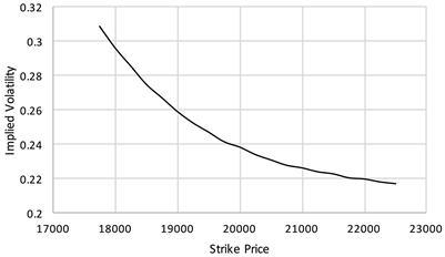
Figure 1. Implied volatility curve for the BS model (4.1).

Figure 2. Implied volatility curve for the Heston model (4.2) under the uncorrelated case, i.e. .

Figure 3. Implied volatility curve for the Heston model (4.2) under the correlated case, i.e. .
price. Furthermore, this phenomenon is observed both with and without stochastic volatility. This implies that a pricing method reflecting the risk-aversion of the market participants generates volatility skewness as mentioned in previous studies.
5. Summary
In this study, we consider the equilibrium pricing for an option. We endo- genously derive a pricing kernel from the market equilibrium of the option and depict, via numerical implementation, that the implied volatility is skewed. In previous studies, other properties of this stylized fact (e.g. anomaly of the option return, U-shaped form of the pricing kernel, etc.) for the option market have been verified. Therefore, in future work, we would like to investigate whether our pricing kernel describes these characteristics.
Cite this paper
Takino, K. (2018) On the Economic Premium Principle. Theoretical Economics Letters, 8, 514-523. https://doi.org/10.4236/tel.2018.83036
References
- 1. Goutte, S., Ismail, A. and Pham, H. (2017) Regime-Switching Stochastic Volatility Model: Estimation and Calibration to VIX Options. Applied Mathematical Finance, 24, 38-75. https://doi.org/10.1080/1350486X.2017.1333015
- 2. Heston, S. (1993) A Closed-Form Solution for Options with Stochastic Volatility, with Application to Bond and Currency Options. Review of Financial Studies, 6, 327-343. https://doi.org/10.1093/rfs/6.2.327
- 3. Hull, J. and White, A. (1987) The Pricing of Options on Assets with Stochastic Volatilities. Journal of Finance, 42, 281-300. https://doi.org/10.1111/j.1540-6261.1987.tb02568.x
- 4. Mondal, M.K., Alim, A., Rahman, F. and Biswas, H.A. (2017) Mathematical Analysis of Financial Model on Market Price with Stochastic Volatility. Journal of Mathematical Finance, 7, 351-365. https://doi.org/10.4236/jmf.2017.72019
- 5. Nicolato, E. and Venardos, E. (2003) Option Pricing in Stochastic Volatility Models of the Orstein-Uhlenveck Type. Mathematical Finance, 13, 445-466. https://doi.org/10.1111/1467-9965.t01-1-00175
- 6. Dupire, B. (1994) Pricing with a Smile. Risk, 7, 18-20.
- 7. Gatheral, J. (2006) The Volatility Surface (A Practitioner’s Guide). Wiley, New Jersey.
- 8. Bakshi, G., Kapadia, N. and Madan, D. (2003) Stock Return Characteristics, Skew Laws, and the Differential Pricing of Individual Equity Options. Review of Financial Studies, 16, 101-143. https://doi.org/10.1093/rfs/16.1.0101
- 9. Christoffersen, P., Heston, S. and Jacobs, K. (2013) Capturing Option Anomalies with a Variance-Dependent Pricing Kernel. Review of Financial Studies, 26, 1963-2006. https://doi.org/10.1093/rfs/hht033
- 10. Yamazaki, A. (2017) A Dynamic Equilibrium Model for U-Shaped Pricing Kernels. Working Paper Series in the Research Institute for Innovation Management, Hosei University, No. 173. https://doi.org/10.1080/14697688.2017.1388535
- 11. Cochrane, J.H. (2005) Asset Pricing (Revised Edition). Princeton University Press, New Jersey.
- 12. Buhlmann, H. (1980) An Economic Premium Principle. Austin Bulletin, 11, 52-60. https://doi.org/10.1017/S0515036100006619
- 13. Iwaki, H., Kijima, M. and Morimoto, Y. (2001) An Economic Premium Principle in a Multiperiod Economy, Insurance. Mathematics and Economics, 28, 325-339. https://doi.org/10.1016/S0167-6687(00)00081-0
- 14. Iwaki, H. (2002) An Economic Premium Principle in a Continuous-Time Economy. Journal of the Operations Research Society of Japan, 45, 346-361.
- 15. Kijima, M., Maeda, A. and Nishide, K. (2010) Equilibrium Pricing of Contingent Claims in Tradable Permit Markets. Journal of Futures Markets, 30, 559-589.
- 16. Takino, K. (2016) An Equilibrium Pricing for OTC Derivatives with Collateralization. Application of Economic Premium Principle. The Soka Economic Studies, 45, 61-72.
- 17. Takino, K. (2017) An Equilibrium Model for an OTC Derivative Market under a Counterparty Risk Constraint. Working Paper. http://www.nucba.ac.jp/university/library/discussion-paper/entry-16991.html