Applied Mathematics, 2010, 1, 124-127
doi:10.4236/am.2010.12016 Published Online July 2010 (http://www.SciRP.org/journal/am)
Problem of Determining the Two-Dimensional Absorption
Coefficient in a Hyperbolic-Type Equation
Durdimurat K. Durdiev
Bukhara State University, Bukhara, Uzbekistan
Received March 25, 2010; revised May 16, 2010; accepted May 29, 2010
Abstract
The problem of determining the hyperbolic equation coefficient on two variables is considered. Some addi-
tional information is given by the trace of the direct problem solution on the hyperplane x = 0. The theorems
of local solvability and stability of the solution of the inverse problem are proved.
Keywords: Inverse Problem, Hyperbolic Equation, Delta Function, Local Solvability
1. Statement of the Problem and the Main
Results
We consider the generalized Cauchy problem
2
<0
(, )=(, ), (, ), >0,
0,
tt xxt
t
uu bxtuxtsxtRs
u
  
 (1)
where ()δ
x
,t is the two-dimensional Dirac delta func-
tion, ()bx,t is a continuous function,
s
is a problem
parameter, and ()ux,t,s . We pose the inverse problem
as follows: it is required to find absorption coefficient
()bx,t if the values of the solution for are known, i.e., if
the function
(0)( )00u,t,sft,s, t, s.
(2)
Definition. A function ()bx,t such that the solution of
problem (1) corresponding to this function satisfies rela-
tion (2) is called a solution of inverse problem (1), (2).
The inverse problem posed in this paper is two-dim-
ensional. For the case where (,) ()bxt bx the solv-
ability problems for different statements of problems
close to (1), (2) were studied in [1] (Chapter 2) and [2]
(Chapter 1). The solvability problems for multidimen-
sional inverse problems were considered in [2] (Chapter
3), [3,4], where the local existence theorems were proved
in the class of functions smooth one of the variables and
analytic in the other variables. In [5], the problems of
stability and global uniqueness were investigated for
inverse problem of determining the nonstationary poten-
tial in hyperbolic-type equation. In this paper, we prove
the local solvability theorem and stability of the solution
of the inverse problem (1), (2).
Let
:{(,)|0 },
T
QtsstT


Ω:{(,)|0|| ||}, 0
Txtxt TxT

 
,
1()
tT
CQ is the class of function continuous in
s
, con-
tinuously differentiable in
t
, and defined on T Q. We
let B denote the set of function )( tx,b such that
(,) (Ω)
T
bxt C

, (,) (,)bxt bxt .
Theorem 1. If at a 0T 1
(,) ()
T
f
tsCQ and the
condition
1
(0,)
2
fs s

 (3)
is met, then for all 00
(0,_0), (1/40),TT Tα

 0 α

()
4(,)
T
'
tCQ
fts the solution to the inverse problems (1),
(2) in the class of function (,)bxt B exists and is
unique.
Theorem 2. Let the conditions in Theorem 1 hold for
the functions (,), 1,2,
k
fts k

and let (,), 1,2,
k
bxt k

be the solutions to the inverse problems with the data
(,), 1,2,
k
fts k

respectively. Then the following esti-
mate is valid for 00
(0, ), ( () TTT

is defined in the
same way as in proof of the Theorem 1)
1
12 12
(Ω)()
4
(,)(,)(,)(,)
1-
TtT
CCQ
bxtb xtftsf ts
ρ
, (4)

D. K. DURDIEV ET AL.
125
where .
T
T
0
 
2. Construction of a System Integral
Equations for Equivalent Inverse
Problems
We represent the solution of problem (1) as
1
(,,)(| |)(,,).
2
uxts θts xvxts (5)
where 1)( t

for ,0t ,0)( t

for 0t

, (,vx
,)ts is a some regular function.
We substitute the Expression (5) in (1), take into ac-
count that (||)/2ts x

 satisfies (in the generalized
sense) the equation () ()
tt xx
uu δxδts

 
, and obtain
the problem for the function
v
:
2
,0
1
(,)(||)(,,),
2
(,) , 0,
0.
tt xxt
t
vv bxtδts xvxts
xt Rs
v

 




(6)
It follows from the d’Alembert formula that the solu-
tion of problem (6) satisfies the integral equation
Δ(,)
2
11
(,,)(,) (||)(,,)
22
, (,) , 0,
t
xt
vxts bξτδτ sξvξτ
s
dξdτxt R s






(7)
where  .,0),(),( txtxxttx  
We use the properties of the

- function and easily ob-
tain the relation in a different form:
()
2
()
2
(,,)
1
(,,)(, )
4
1
(, )(,,),
2
,
xts
xts
t
Υxts
vxts bξsξdξ
bξτvξτsdτdξ
ts x






 (8)
where the domain (,,)
x
ts

is defined by
()
(,,) (,),2
,0,.
2
x
ts
xtsst x
xts
s
ts const

 





 
 

By differentiating the equality (8), we obtain
()
2
()
2
1
(,,) ,
82 2
,
22
1(, )(, , ), .
2
t
xts
t
xts
xtsxts
vxts b
xts xts
b
btxv txsdtsx








 





 

(9)
It is obvious that 1
(,)(0,,)(0,,)
2
f
tsu tsv ts
for 0t. Moreover, the function (, )
f
ts be must sat-
isfy the condition (9).
We set 0x

in the equality (9), use the fact that the
function (,)bxt is even in
x
, and obtain the relation

2
2
1
(,),
422
,, , ,
(,) .
t
ts
t
ts
T
tsts
ftsb
bξtξvξtξsdξ
ts Q










We rewrite this equality, replacing ()/2ts with
||
x
and ()/2ts

with t, and solve it for (,).bxt We
obtain

-
(,)4(||, ||)4,
(, ||, ||), ||.
x
'
t
x
t
bxtftx txbξtxξ
vξtxξtxdξtx

 
 
(10)
Let


(,,) ,0
T
x
tsxs t Txs tT


 
The domain T

in the space of the variables ,,
x
t
and
s
is a pyramid with the base t  and vertex
(0,,/2)TT . To find the value of the function b at (,)
x
t,
it is hence necessary to integrate (,)bxt over the inter-
val with the endpoints (| |,)
x
t

and (||, )
x
t and to
integrate the function (,,)
t
vxtsover the interval with
the endpoints (||, ,||)
x
tt x

 and (||,,||),
x
tt x

which belong to the domain T

.
One can rewrite the system of Equations (9) and (10)
in the nonlinear operator form,
,


A (11)
where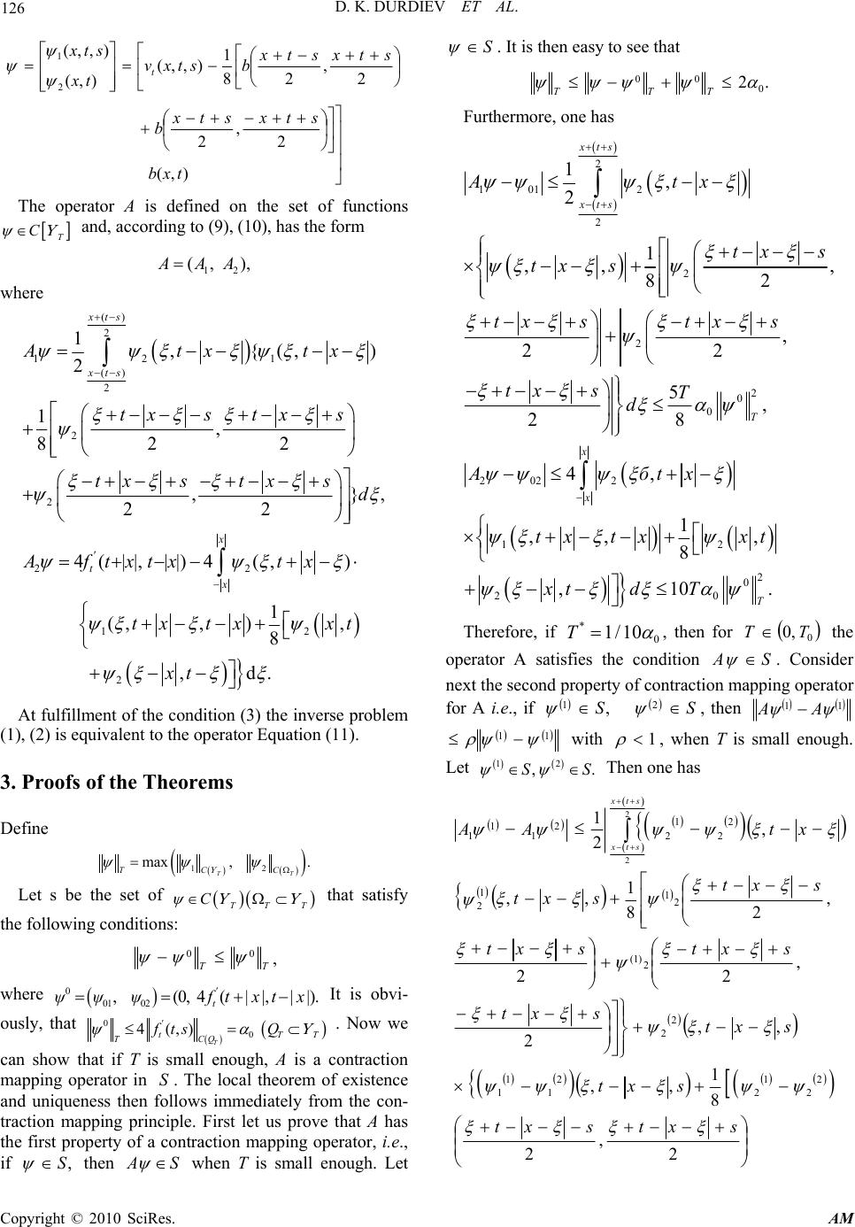

D. K. DURDIEV ET AL.
126



































),(
2
,
2
2
,
28
1
),,(
),(
),,(
2
1
txb
stxstx
b
stxstx
bstxv
tx
stx
t



The operator A is defined on the set of functions


T
C

  and, according to (9), (10), has the form
12
(, ),
A
AA
where


()
2
12 1
()
2
2
2
22
12
1,{(,)
2
1,
82 2
,},
22
4(||, ||)4(,)
1
(,,),
8
xts
xts
x
'
t
x
Atxtx
txstxs
txstxs d
Aftxtx tx
tx txxt

 






 









 





 

 






2
,d.xt  



At fulfillment of the condition (3) the inverse problem
(1), (2) is equivalent to the operator Equation (11).
3. Proofs of the Theorems
Define
 

12
max ,.
TT
TCC 



Let s be the set of

 
TT T
C

 
that satisfy
the following conditions:
TT
00
 ,
where


0
01 02
, (0, 4(||, ||).
'
t
ψψψ
f
txtx
It is obvi-
ously, that



0
0
4(,)
T
'
tTT
TCQ
fts Q  
. Now we
can show that if T is small enough, A is a contraction
mapping operator in S. The local theorem of existence
and uniqueness then follows immediately from the con-
traction mapping principle. First let us prove that A has
the first property of a contraction mapping operator, i.e.,
if ,S

then SA 

when T is small enough. Let
S


. It is then easy to see that
.20
00
  TTT
Furthermore, one has









2
1012
2
2
2
2
0
0
202 2
12
2
1,
2
1
,, ,
82
,
22
5,
28
4,
1
,,,
8
,10
xts
xts
T
x
x
Atx
txs
tx s
tx stx s
tx sT
d
Aбtx
tx txxt
xt d
 

 
 


 
 
 



 













 

 


 





 



2
0
0.
T
T 
Therefore, if *
0
1/10T

, then for


0
,0 TT  the
operator A satisfies the condition SA 

. Consider
next the second property of contraction mapping operator
for A i.e., if




SS

21 ,


, then




11
 AA 




11
  with 1


, when T is small enough.
Let




12
,.SS


 Then one has
  
  




 



 


 
 






















 



















 


2
,
2
8
1
,,
,,
2
,
22
,
28
1
,,
,
2
1
2
2
1
2
2
1
1
1
2
2
2
)1(
2
1
1
2
2
2
1
2
2
1
1
1
2
2
sxtsxt
sxt
sxt
sxt
sxtsxt
sxt
sxt
xt AA
stx
stx












D. K. DURDIEV ET AL.
127
 

 
12
22
12
0
,
22
5,
2T
tx stx s
T
d








  





  







 



 



 


 


 
 
12 12
22 22
1
1
1(1)
22
212
211
11
22
11
22
12
0
4
, ,,
1 , ,
8
,
1
,,
8
, ,
40 .
x
x
T
AA
txtxtx
xt xt
tx
tx tx
xt xt
dT 
 
  




 




 
 



 

 


 



It follows from the preceding estimates that if

0
0401
T, then for


0
,0 TT  the operator A is a
contraction operator with 0 /TT

on the set S.
Therefore, the Equation (11) has a unique solution which
belongs to S according to the contraction mapping prin-
ciple. The solution is the limit of the sequence



n,
0,1,2,...,n where






  
nn A 10 ,0, and
the series


 
0
10
n
nn

converges not slower than the series
  
T
n
n
T 
0
010
 
We now prove Theorem 2. Since the conditions
Theorem 1 hold, the solution belong to the set S and
.2,1,2 0 i
T
i
 Let


2,1, k
k
 be vector
functions which are the solution of the Equation (11)
with the data


,, 1,2,
k
fts k respectively, i. e.,





kk A

From the previous results in the proof of Theorem 1, it
follows that

  

12
12 1
012
,,4 ,,
40,1, 2.
kk
Q
CtT
T
xtsf tsfts
Tk





Therefore, one has




1
12 12 12
4, ,
TT
t
fts ftsQ
CT
  




 
The last inequality gives
 
1
12 12
4,,
1
Tt
fts ftsQ
CT
 




 
 (12)
The stability estimate (4) follows from the inequality
(12).
4. References
[1] V. G. Romanov, “Inverse Problems of Mathematical
Physics,” in Russian, Publishing House “Nauka”, Mos-
cow, 1984.
[2] V. G. Romanov, “Stability in Inverse Problems,” in Rus-
sian, Nauchnyi Mir, Moscow, 2005.
[3] D. K. Durdiev, “A Multidimensional Inverse Problem for
an Equation with Memory,” Siberian Mathematical Jour-
nal, Vol. 35, No. 3, 1994, pp. 514-521.
[4] D. K. Durdiev, “Some Multidimensional Inverse Prob-
lems of Memory Determination in Hyperbolic Equa-
tions,” Journal of Mathematical Physics, Analysis, Ge-
ometry, Vol. 3, No. 4, 2007, pp. 411-423.
[5] D. K. Durdiev, “Problem of Determining the Nonstation-
ary Potential in a Hyperbolic-Type Equation,” Journal of
Theoretical and Mathematical Physics, Vol. 2, No. 156,
2008, pp. 1154-1158.