Agricultural Sciences
Vol.3 No.4(2012), Article ID:20100,18 pages DOI:10.4236/as.2012.34074
Outlook of future climate in northwestern Ethiopia
![]()
1College of Agricultural and Environmental Sciences, Haramaya University, Haramaya, Ethiopia; *Corresponding Author: derejeayal@yahoo.com
2College of Agricultural and Environmental Sciences, Bahir Dar University, Bahir Dar, Ethiopia
3Ethiopian Institute of Agric-Research, Coordinator, National Agro meteorology Research, Nazreth, Ethiopia
4Amhara Region Agricultural Research Institute, Bahir Dar, Ethiopia
5ICARDA-Ethiopia National Project Officer International Center for Agricultural Research in the Dry Areas, Bahir Dar, Ethiopia
Received 20 March 2012; revised 26 April 2012; accepted 10 May 2012
Keywords: Amhara Regional State; Climate change; Ethiopia; HadCM3; Statistical Downscaling
ABSTRACT
Climate change is described as the most universal and irreversible environmental problem facing the planet Earth. Whilst climate change is already manifesting in Ethiopia through changes in temperature and rainfall, its magnitude is poorly studied at regional levels. The objective of this study was to assess and quantify the magnitude of future changes of climate parameters using Statistical Downscaling Mode (SDSM) version 4.2 in Amhara Regional State which is located between 8˚45(N and 13˚45(N latitude and 35˚46(E and 40˚25(E longitude. Daily climate data (1979- 2008) of rainfall, maximum and minimum temperatures were collected from 10 observed meteorological stations (predictand). The stations were grouped and compared using clustering method and Markov chain model, whereas the degree of climate change in the study area was estimated using the coupled HadCM3 general circulation model (GCM) with A2a emission scenarios (Predictors). Both maximum and minimum temperatures showed an increasing trend; and the increase in mean maximum and minimum temperature ranges from 1.55˚C - 6.07˚C and from 0.11°C - 2.81°C, respectively in the 2080s compared to the base period considered (1979- 2008). The amount of annual rainfall and number of rainy days also decreased in the study Regions in the 2080s. The negative changes in rainfall and temperature obtained from the HadCM3 model in the current study are alarming and suggest the need for further study with several GCM models to confirm the current results and develop adaptation options.
1. INTRODUCTION
Climate has profound effects on the biophysical resources of the planet. It is the major factor controlling the patterns of vegetation structure, productivity, and plant and animal species composition [1]. Many plants can successfully reproduce and grow only within a specific range of temperature and respond to specific amounts and seasonal patterns of rainfall, and fail to survive if climate changes. Thus, there is now a substantial concern over the global problem of climate change and its current and future impacts. The impact of changing climate, such as rising global average temperatures and increases in frequency and severity of extreme events, droughts and floods, are already affecting human well-being, biodiversity and ecosystems, economies and societies worldwide [2]. Seasons are shifting, temperatures are climbing and sea levels are rising around the globe. Meanwhile, our planet must still supply us and all living things with air, water, food and safe places to live [3].
Africa contains one-fifth of all known species of plants, mammals, and birds, as well as one-sixth of amphibians and reptiles. However, because of climate change, these ecosystems are threatened [4,5]. Similarly, the varied ecology, edpahic and climatic conditions in Ethiopia which accounts for the wide diversity of biological resources both in terms of flora and fauna is declining because of climate variability [5,6]. The negative impacts associated with climate change are also compounded by many factors, including widespread poverty, human diseases, and high population density, which is estimated to double the demand for food, water, and livestock forage within the next 30 years [7]. For example; climate variability and extreme weather events, such as high temperatures and erratic rainfall, are critical factors in initiating malaria epidemics and increase the spread of infectious diseases especially in the highlands of Ethiopia [3,8,9]. In addition, [10,11] noted that rainfall variability and associated droughts have historically been major causes of food shortages and famines in Ethiopia.
Being able to predict seasonal climate can help to mi-nimize the possibility of “climate surprises” in order to reduce impacts to society and ecosystems. With these predictions, decision makers can be provided with reliable scientific information about possible extreme climate events. Many sectors of society use these predictions, including agriculture, fishing, forestry, energy, insurance, public health, water resources, recreation, transportation, health, and construction. For example, with an increased risk of drought, we know that some possible impacts include water shortages, early onset of the wildfire season, and lower or no crop yields. This in turn could lead to increased disaster assistance payments, higher food prices, and disrupted transportation on internal waterways. With advance knowledge of drought, water resource managers can adjust the timing of water releases from reservoirs, and farmers can alter the type of crops they plant [12].
While most of us feel the effects of climate variation, many businesses, services and activities depend on climate prediction to prepare adequately, to manage risk, protect the environment, and to save lives [13]. A prediction process, begins with observing and accurately measuring the most recent and current environmental conditions. The tools of the predictor can therefore be based on statistics from historical climate data which have been analyzed to show the relationships between the Earth’s surface conditions and climate [12].
Numerical models (General Circulation Models or GCMs), are currently most credible tools available for simulating the response of the global climate system [14]. However, because of their coarse spatial resolution, GCMs to date are unable to provide reliable climatic information at regional and local scales [15]. As suggested in different guidelines and documentation developed by the IPCC [16,17], the climate change information required for many impact studies is at a much finer spatial scale than that provided by GCMs. Because of this limitation, other alternative methods called down-scaling techniques using statistical downscaling model (SDSM) have been developed in recent years to obtain fine resolution climate change information at regional/local scales. The SDSM calculates statistical relationships, based on multiple linear regression techniques, between large-scale (the predictors) and local (the predictand) climate [15]. These relationships are developed using observed climate data and, assuming that these relationships remain valid in the future, and hence can be used to obtain downscaled local information for some future time period by driving the relationships with GCM-derived predictors [16,18,19].
Hadley Centre Coupled Model (HadCM3) outputs established on the A2 scenario is the most commonly used GCM to develop climate change scenarios in a given area and regional impact assessment studies [20, 21]. Its good simulation of current climate without using flux adjustments was a major advance at the time it was developed and it still ranks highly compared to other models [22]. Hence, HadCM3 was one of the major models used in the IPCC Third and Fourth Assessments. Further, (e.g. [23]) used HadCM3 models in order to develop climate change scenarios of rainfall, minimum and maximum temperatures in arid regions of Chile in order to analyze the future potential impact of climate change on stream flow. In addition, HadCM3 GCM model out-puts established on the A2 scenario was used to downscale climate change scenarios at regional levels [24]. Further more, [25] also used the outputs of HadCM3 A2a and B2a scenarios for climate change impact analysis using crop modeling.
Accurate and timely climate information and predictions can help many sectors of society circumvent the impacts posed by climate variations. This reduces the risk of economic setbacks and ecological damage. Therefore, the aim of this paper was to downscale and quantify the magnitude of future changes of maximum and minimum temperatures and rainfall at a local level in the Amhara Regional State using the HadCM3A2a GCM models.
2. MATERIALS AND METHODS
2.1. Description of the Area
Amhara region is located between 8˚45¢N and 13˚45¢N latitude and 35˚46¢E and 40˚25¢E longitude in North West Ethiopia. The total area of the region is estimated at 156,960 km2, which is divided into 11 administrative zones and 105 districts [26] (see Figure 1).
2.2. Climate of the Study Area
The climate of the Amhara Region is affected significantly by variation in altitude, its latitudinal position, prevailing winds, air pressure and circulation and its proximity to the sea. Traditionally, the climate of the Region is divided in to Kola (hot zone) which represents and cover 31% of the Region with altitude below 1500 meters above sea level (a.s.l.) and Woyina Dega (warm zone) which covers 44% of the Region encaompasses areas between 1500 - 2500 m a.s.l and Dega (cold zone) which covers 25% of the Region representing areas between 2500 - 4620 m a.s.l [9]. The annual mean temperature of the Region is between 15˚C and 21˚C. But in valleys and marginal areas the temperature exceeds 27˚C [27].
3. DATA SETS AND METHODOLOGY
3.1. Observed Data
Thirty years observed rainfall data (1979-2008) was
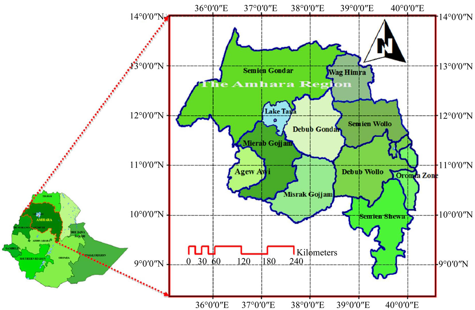
Figure 1. Geographical location of Amhara Regional State with reference to national map of Ethiopia.
collected from National Meteorological Agency (NMA) of Ethiopia for 10 meteorological stations in the Amhara region. The meteorological stations were clustered by hierarchical clustering method with quantitative data set and Squared Euclidean Distance with wards methods using StatistiXL software.
3.2. General Circulation Model Data (GCM)
The GCM data were collected from the IPCC Data Distribution Center (DDC) which was established in 1998 by the World Metrological Organization and the United Nations Environmental Program, following a recommendation by the task group on Data and Scenario Support for Impact and Climate Assessment [28]. However, because the daily fields are only available directly from the respective modeling centers, the climatic data used for SDSM had been collected from the Canadian Institute for climate studies website for model output of HadCM3 [29]. The predictor variables were supplied on a grid basis of size 2.5˚ latitude × 3.75˚ longitude so that the data were downloaded from the nearest grid box to the study area.
As shown in Figure 2, Hence the nearest grid box for the HadCM3 model, which represents the study area, is the one at 10.95˚N latitude and 37.85˚E longitude (Y = 31 Latitude 10˚N and X = 12 Longitude 41.25˚E).
3.3. Baseline Period Data
One of the criteria used in evaluation of the performance of any useful downscaling method is whether the historic (observed) condition can be replicated or not [16]. It is therefore imperative that the methods used for transforming the results of climate models to meteorological stations will generate precipitation rainfall and temperature series that should have the same statistical properties as observed meteorological data for use in climate modeling [30]. The years from 1/1/1979 to 31/ 12/2008 were used as a baseline period for the study [5]. Thus, the HadCM3 data were downscaled for the baseline period A2 emission scenarios and the statistical properties (mean and variance) of the downscaled data were compared with observed data of the same period.
4. METHODS OF CLUSTERING ANALYSIS AND HOMOGENITY TEST
4.1. Clustering Analysis
Clustering (or numerical classification) uses a data array, or matrix, to classify (or cluster) the cases (rows) of data into groups according to values of their attributes (columns). Geographical location (latitude, longitude and elevation) and climatologically mean monthly rainfall (1979-2008) of all stations were used to calculate their standardized standard deviation. Hence using Hierarchical Clustering method the stations were grouped; there was no prior knowledge of grouping (or any prior grouping was ignored). The data were separated data into groups based on individual cases using clustering analy sis [31]. Therefore, the data was summarized and stations were grouped using tree graph (dendrogram) (Figure 3).
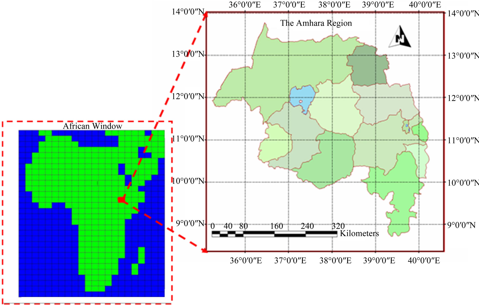
Figure 2. The African continent window with 2.5˚ latitude × 3.75˚ longitude grid size from which the grid box for the study area was selected (shown in red/or back if printed in black and white).
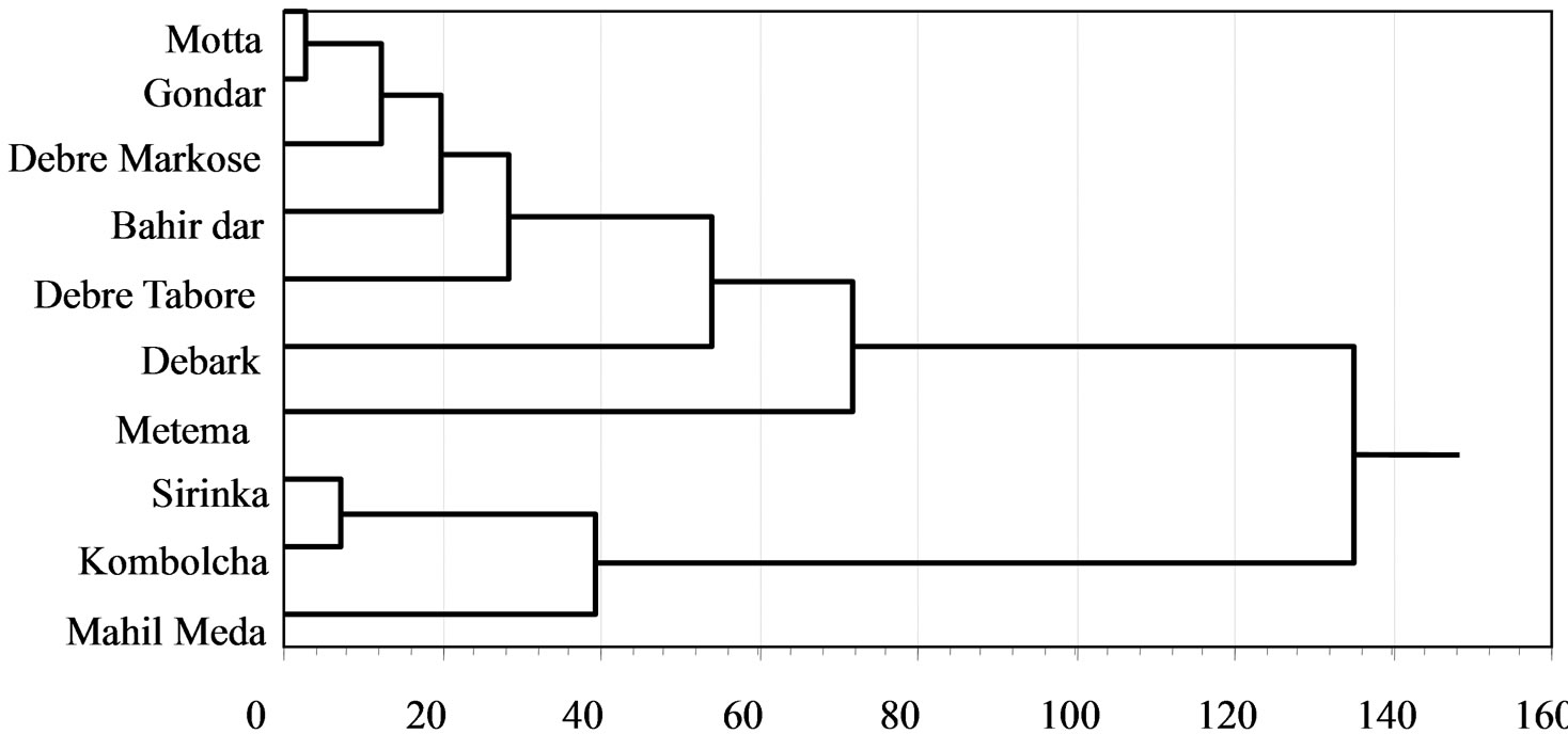
Figure 3. Dendrogram of meteorological stations in the Amhara Regional State.
4.2. Selection of Representative Station
Since the downscaling method is statistical using a site specific tool called SDSM, there was a need to select one representative station which was statistically correlated with the rest of the stations in each cluster. According to [31], the software StatistiXL was used for clustering partial correlation of each station belonging to each group and the software gave all statistical tests needed. The station with better correlation coefficient in each group was selected for the study.
4.3. Homogeneity Test
Markov chain model is one of the facilities in Instat + V3.36 for fitting the probabilities of rain and to the rainfall amounts. A model was first fitted to the chance of rain and then to the amounts. First order Markov chain model [32], uses the probability of rain or dry day in the given observational data. a threshold value 0.1 mm/day was used as dry day and all days with rainfall value greater than this value were considered as rainy day. Following this it was possible to examine whether all the stations in each cluster have similar rainfall seasons or not. Moreover, first order Markov chain model clearly gave the probability of getting rain on a daily basis and the chance of getting rain in each season [32]. This was used to identify the dry and rainy seasons of each cluster in the study area.
The zero order Markov chain model was used for testing the homogeneity while first order was used to fill missing daily rainfall values. The main reason to select the first order to fill the missing data rather than second order was that first order didn’t exaggerate the resulting values and gave more accurate model to each cluster of the study area as explained by the National Meteorological Agency of Ethiopia [33].
4.4. Settings of the SDSM
According to [16], the concept of regional climate being conditioned by the large-scale state may be written as:
R = F (L)
whereR represents the predicted (regional or local climate variables)L represents the predictor (a set of large-scale climate variables)F is a deterministic/Stochastic function conditioned by L and has to be found empirically from observed or modeled data sets.
The climate scenario for future period were developed from statistical downscaling using GCM HadCM3 predictor variable for the emission scenarios for 100 years based on the mean of 20 ensembles; and the analyses was done based on three 30-years periods centered on the 2020s (2011-2040), 2050s (2041-2070) and 2080s (2071- 2099).
4.5. Settings Used for SDSM
For the observed and the National Centre for Environmental Prediction (NCEP) data the year length was set to be the default (366 days), which allows 29 days in February in leap years. However, as HadCM3 have modeled years that do only consist of 360 days, the default value was changed to 360 days. The base period used for the model was from 1/1/1979 to 31/12/ 2008.
T he event threshold value is important to treat trace values during the calibration period. For the temperature parameter, this value was set to be 0 while for daily rainfall calibration purpose this parameter was fixed to be 0.1 mm/day so that trace rain days below this thresh-old value were considered as a dry day. Missing data were replaced by –999.
For the daily temperature values, no transformation was used as it is normally distributed and the model was non-conditional. However, for the daily rainfall, the fourth root transformation was used as its data were skewed and as its model was conditional. The range of variation of the downscaled daily weather parameters was controlled by fixing the variance inflation. The default value, which is 12, was used for the daily temperature values; where as for daily precipitation this value was set as 18, in order to magnify the variation. The bias correction, which compensates for any tendency to over or underestimate the mean of conditional processes by the downscaling model, was set to be 0.8 for daily rainfall, and the default 1.0 for daily temperature (indicating no bias correction).
4.6. Steps Used in SDSM Model Approach
Data were checked for their quality; gross data errors, missing data codes and outliers were identified prior to model calibration. Predictors and/or the predictand were also transformed. Then, empirical relationships between gridded predictors and single site predictands (station precipitation) were identified; the selection was done at most care as the behavior of the climate scenario completely depends on the type of the predictors selected. After this, models were calibrated and results for the different time slices were developed. Calibrated models (using independent data) and the synthesis of artificial time series data representing current climate conditions were verified. Then both derived SDSM scenarios and observed climate data were interrogated with the analyses data screen of SDSM and monthly statistics produced were plotted using the compare results screen. Then, rapid assessment of downscaled versus observed, and/or current versus future climate scenarios were compared.
Finally, the outputs of the Hadley Centre Coupled Model (HadCM3) with A2a scenario, which is the most commonly used GCM for downscaling future climate of an area (e.g. [23]), were used to develop climate change scenarios in the region.
According to [16], the regression weights produced during the calibration process were applied to the time series outputs of the GCM model. This is based on the assumption that the predictor-predictand relationships under the current condition remain valid under future climate conditions too. Twenty ensembles of synthetic daily time series data were produced for A2a SRES scenarios for a period of 139 years (1961 to 2099). The final product of the SDSM downscaling method was then found by averaging the twenty independent stochastic GCM ensembles of A2a and B2a emissions scenarios. Statistical significance of the mean values of maximum and minimum temperatures found at different time scales were tested using a paired t-test mean comparison at 0.05 alpha level.
5. RESULTS AND DISCUSSIONS
5.1. Clustering Analysis
A dendrogram (tree graph) is a common means of graphically summarizing a clustering pattern using Statisti XL. The dendrogram usually starts with all individuals as separate clusters (“tips”) and shows the combination of fusions back to a single “root”. The order of individuals shown in the dendrogram was the order in which the groups enter the clustering [31]. In this study, the maximum distance or similarity to classify as one group is 60 (Figure 3).
All available stations, which were 10 before clustering, were clustered and classified in to three groups and each group was designated as cluster/Region A (Kombolcha, Mahil-Meda and Sirinka), cluster/Region B (Metema) and cluster/Region C (Motta, Gondar, Debre Markose, Debre Tabore and Debark) randomly.
The designation of each cluster was done just to represent climatologically homogeneous areas within the study area (Figure 3). The geographical locations of the stations grouped and the representative clusters used for the study are given in Figure 4. Based on the clusters, climatologically the Amhara region has a mean maximum temperature of 26.0˚C, 35.8˚C and 23.6˚C for cluster A, B and C, respectively, but inter-annual variability of rainfall was observed in all clusters (Figures 5 and 6).
Based on the maximum and minimum temperature data, the mean monthly temperature over the Amhara region tend to increase until the beginning of June in all regions and decreased during the main rainy season ((June to September) (Figure 6)). Contrarily, Tmin had greater value during the main rainy season, and the mean minimum temperature over Amhara region was 11.6˚C,
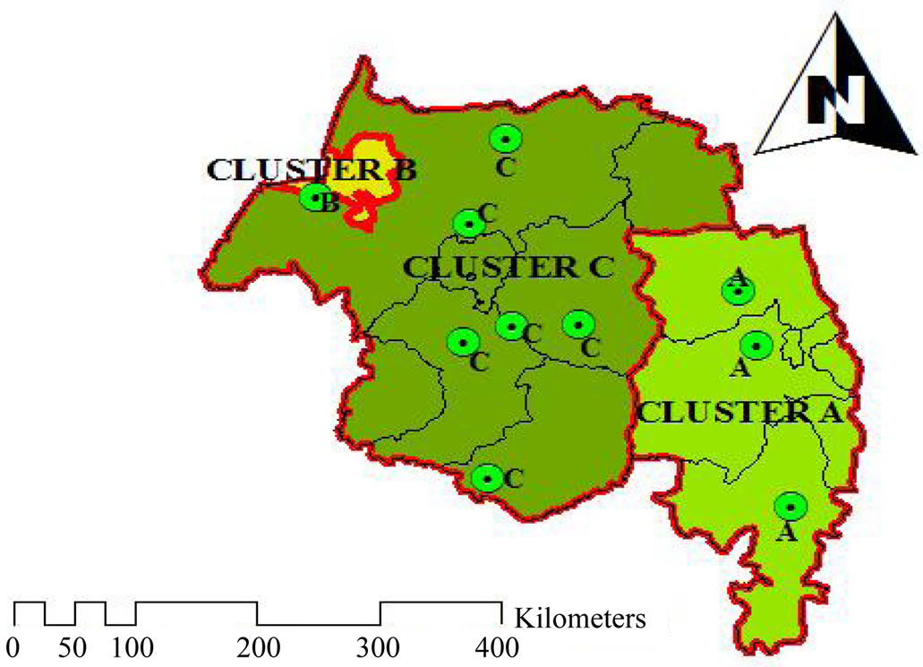
Figure 4. Three climate regions in the Amhara Regional State clustered based on 30 years climate data (1979-2008).
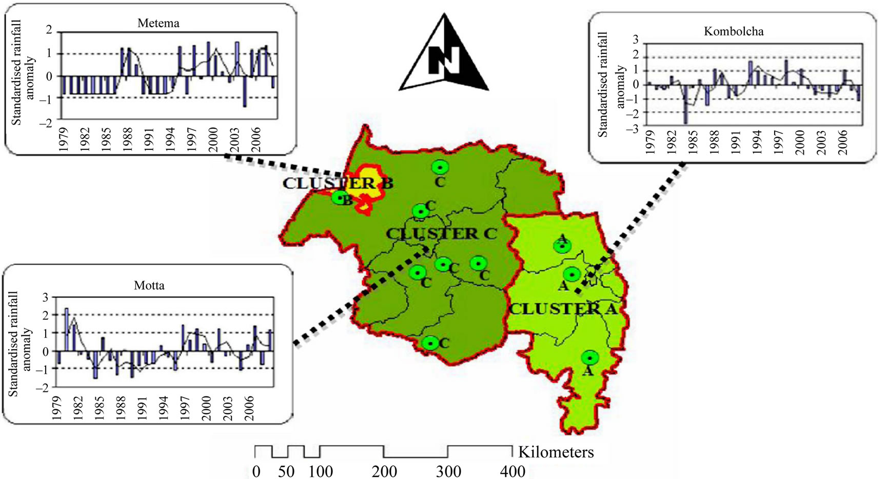
Figure 5. Rainfall variability in three clustered regions in the Amhara Regional State for the period 1979-2008.
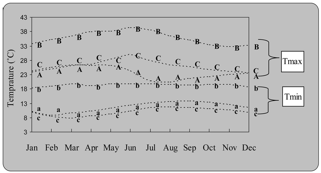
Figure 6. Monthly average temperature of three clustered regions (A, B and C) in the Amhara Regional State for the period 1979-2008. Letters: A, B, C and a, b, c represent respective clusters for maximum and minimum temperatures.
19.3˚C and 10.0˚C for Clusters A, B and C, respectively.
5.2. Homogeneity of Stations
Homogeneity test analysis showed that Cluster C and Cluster B had only one main rainy season. The rainfall in Cluster C is long with early onset and late end date of the rain, while in Cluster B rainfall is characterized by late onset and early cessation of rain (Figure 7).
Cluster A has two rainy seasons which are locally known as “belg” (small rainy season) and “kiremit” (main rainy season). The two rainy seasons have no distinct dry period on their translation; hence, the small rainy season is soon after followed by the main rainy season. In addition, the length of main rainy season is similar to Cluster C.
5.3. Selection Representative Stations
Partial correlations of each station belonging to each group were analyzed. In each group, stations with better correlation coefficient were selected (highlighted with grey/black if it is printed in black and white in Table 1). Kombolcha and Motta meteorological stations had good correlation in their respective Cluster (Table 1). While, Metema meteorological stations didn’t correlate with other observatory stations, hence it stood alone as Cluster B. Henceforth, only these stations were used for further analysis.
These stations were taken as representative of the climate stations with respect to average monthly rainfall (priority was given for rainfall than temperature). Therefore, temperature data was taken from the selected representative station out of respective Cluster of a group. Consequently, the climate scenarios were only developed for these selected stations.
5.4. Predictor Variables Selected
The type and explanations of the predictors, which showed better correlation with the daily maximum temperature, daily minimum temperature, and daily rainfall predictands at p < 0.05 significance level are shown in Table 2. Partial correlations indicate that the corresponding predictor had the strongest association with the predictand.
5.5. Calibration and Validation
The simulated maximum and minimum temperatures in clusters A and C had better agreement with the observed results than rainfall/precipitation (Table 3). Though simulated values of rainfall showed a lesser agreement as compared to the maximum temperature and minimum temperatures in all clusters, the result was quite acceptable due to the fact that precipitation is a conditional process [14]. Conditional processes like precipitation are dependent on other intermediate processes like the occurrence of humidity, cloud cover, and/or wet-days. Unconditional processes like temperature; however, are not regulated by other intermediate processes.
In addition, as indicated in the SDSM manual [14], local temperatures are largely determined by regional forcing whereas precipitation series display more “noise” arising from local factors. Hence, larger differences can be observed in precipitation ensemble members than that of temperature.
On the other hand, the minimum and maximum temperatures over Cluster B simulation showed a very poor agreement with the observed one (Table 3). Even though it is difficult to exactly point out the reason behind, this could be due to low/inferior data quality used for the comparison.
Validation was done based on 15 year simulation from 1993 to 2008. The validation statistics for maximum and minimum temperatures and rainfall in all clusters are shown in Table 4.
The correlation factors that were found during the calibration step are more or less maintained during the validation period too, even better agreement was found here.
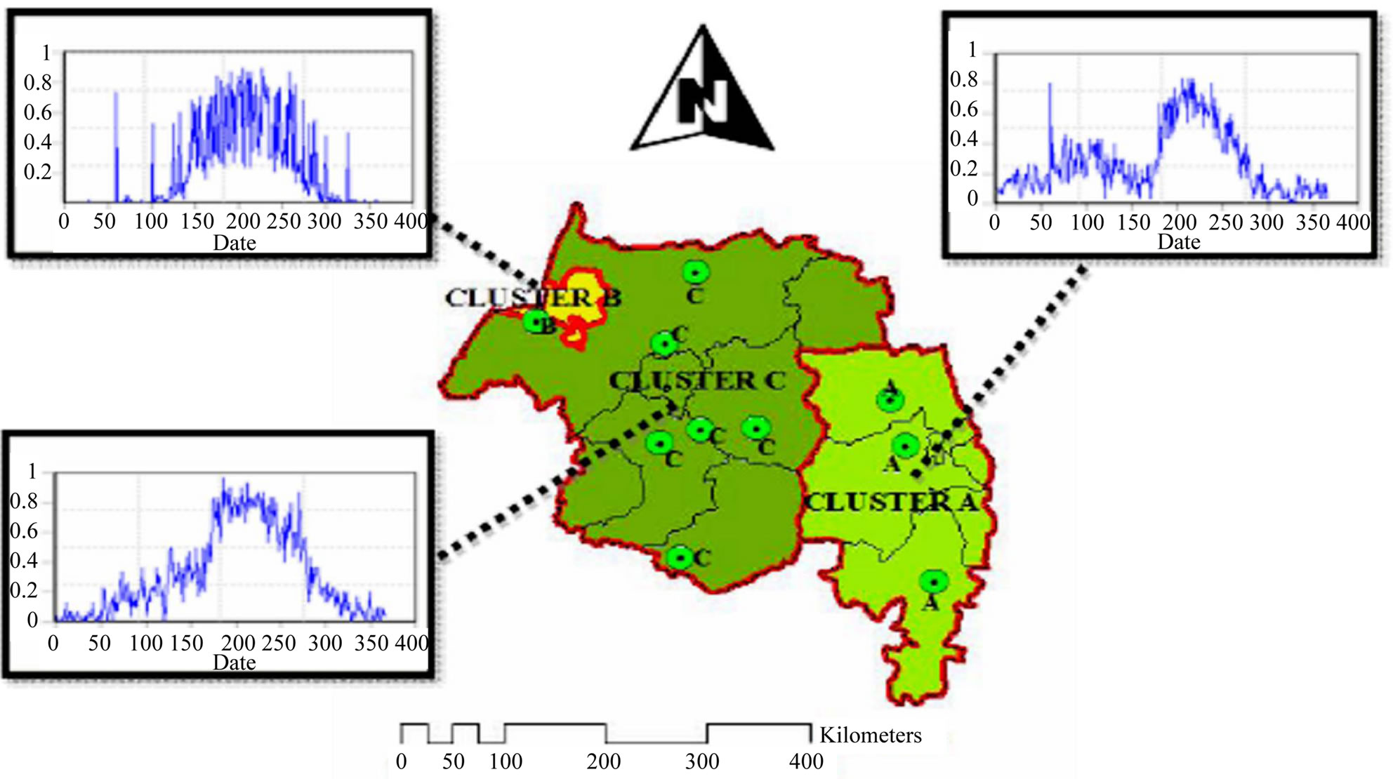
Figure 7. Homogeneity test using Markov chain model (zero order) for three cluster regions in the Amhara Regional State.
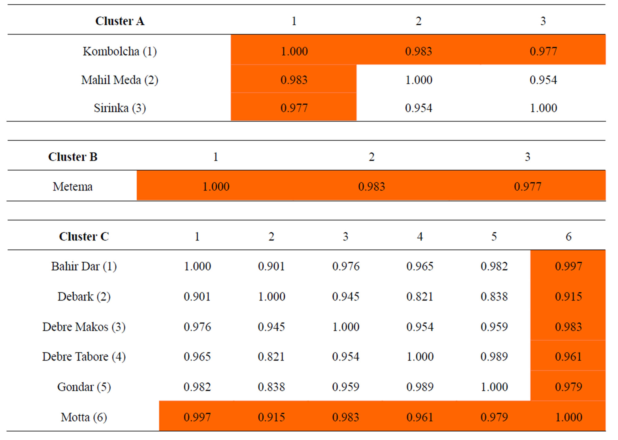
Table 1. Correlation matrix of stations average monthly rainfall in three cluster regions of the Amhara Regional State.
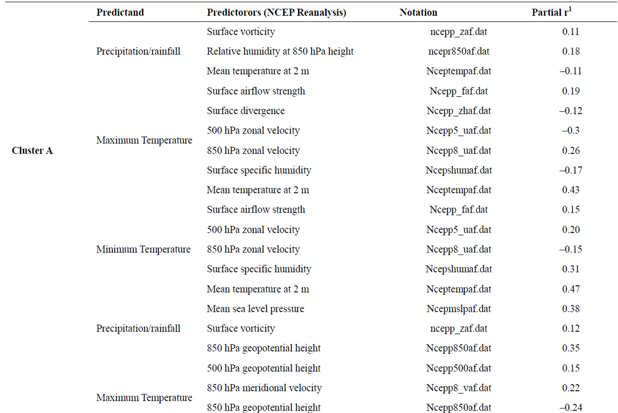
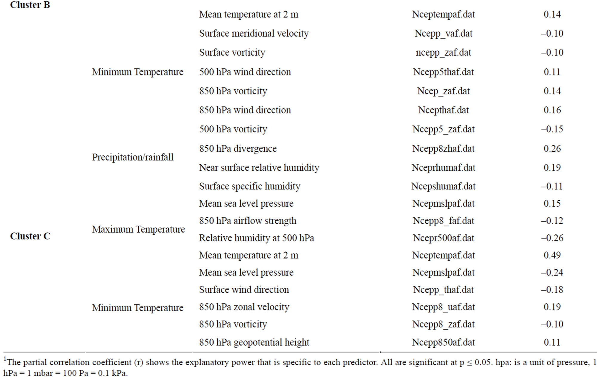
Table 2. List of predictor variables that gave better correlation results at p < 0.05.
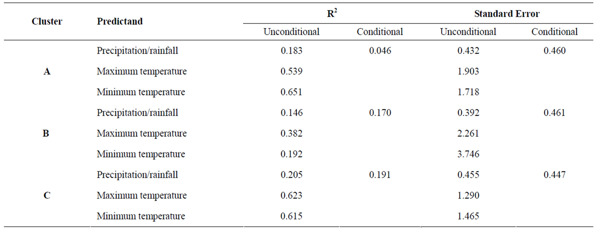
Table 3. Calibration statistics of daily rainfall and maximum and minimum temperatures for three clustered regions in the Amhara Regional State.
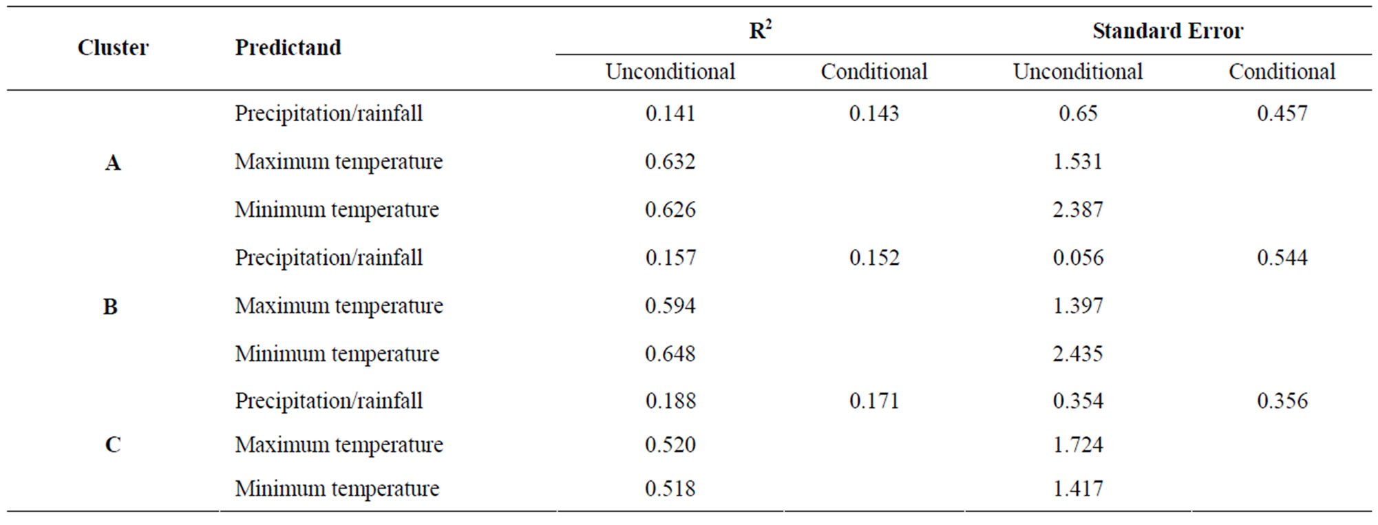
Table 4. Validation statistics of daily rainfall and maximum and minimum temperatures for three clustered regions.
5.6. Projected Climate Changes
According to [34], extensive area specific research conducted in various parts of the world, had concluded that, even a slight warming in average surface temperatures increased the likelihood of extreme weather (hail, lightning, tornadoes, heat waves and/or damaging winds). The findings in this paper also showed similar conditions. Relative to the base climate period of 1979-2008, the statistical downscaled values of SDSM projections for the period 2080s showed that Tmax could rise by up to 2.3˚C, 4.9˚C and 1.8˚C, while rainfall could decrease by 27.2%, 42.3% and 12.2% over Clusters A, B and C, respectively (Table 5); all SDSM downscaled value were significant (p < 0.05). Although this finding provided important information for preparing developmental strategies and policy interventions in the region, the results are based only on oneGCMs output and opns the door for testing the result with more GCM results.
5.7. Analysis of Variability and Extremes of Basic Downscaled Parameters (Tmax, Tmin, and Pcpn)
5.7.1. Daily Maximum Temperature (Tmax)
Temperature is normally distributed [5], and hence the distributions of Tmax and Tmin were examined for changes in mean and variance, and how changes in these two statistics affected the occurrence of records of hot or cold weather. The relevant statistics for Tmax from observed and downscaled data showed there was an increase in mean value of maximum temperature and its variability in Clusters A, B and C. Table 6 shows the increase in mean value of Tmax up to 2.06˚C, 6.07˚C and 1.55˚C with its increase in variability (standard deviation) of about 18.83%, 13.15% and 8.51% in Clusters A, B and C, respectively in the 2080s. This result is in better conformity with [5] that also projected an increase in mean global temperature of up to 5.8˚C by the end of the 21st
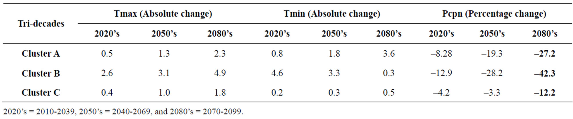
Table 5. Downscaled maximum and minimum temperatures and rainfall in three clustered regions of Amhara Regional State.
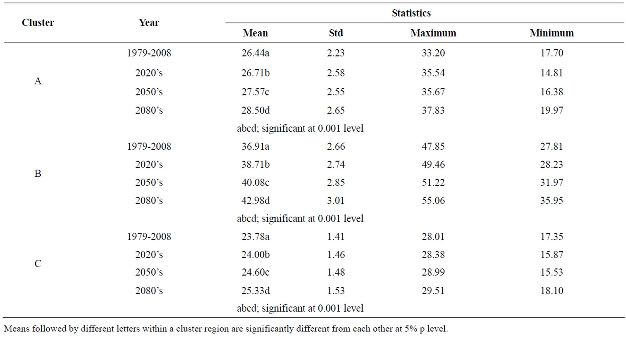
Table 6. Summered statistics mean of maximum temperature in three clustered regions of Amhara Regional State.
century. The possible reason for rise in temperature according to [35] may be associated with the dramatic warming of oceans over the Atlantic and /or Indian oceans which further warm the sea surface temperature in the two oceans and result in low pressure formation in the area and decrease in moist air advection towards Ethiopia.
This might be the case for the increase in number of days with Tmax > 28˚C, Tmax > 30˚C and Tmax > 32˚C in all clusters by 2080’s (Figure 8). Further, [5] reported that climate change may increase the frequency of ENSO warm phases in Africa. The present study also showed the more likely occurrence of heat wave in all clusters for the projected years than before. The projected climate in Cluster A showed that heat wave was more likely to occur starting from 2020’s, and it would be a common weather event for Cluster B. However, Cluster C will stay safe and experiences wave free days even by 2080’s (Figure 8).
5.7.2. Daily Minimum Temperature
The present study revealed that the average daily minimum temperature in Amhara region generally was increasing. For example, a rise in mean daily minimum temperature of about 2.80˚C, 0.11˚C and 0.64˚C are noted in Clusters A, B and C by 2080s, respectively (Table 7). This finding is in agreement with the historical climate of the country. According to [36], annual minimum temperature has been increased by about 0.37˚C every 10 years over the past 55 years. Although, the result in Clusters B and C showed less change in mean minimum temperature than cluster A from the base period, it indicates a shift towards warmer conditions in the future. In general, the projected climate in the three clusters indicated a decreas in the number of cold days (Figure 9)
Days with minimum temperature less than 7˚C are projected to become less common, in all clusters in the future climate scenario (Figure 9). This is in line with [5] and [37] who reported increasing trend in minimum
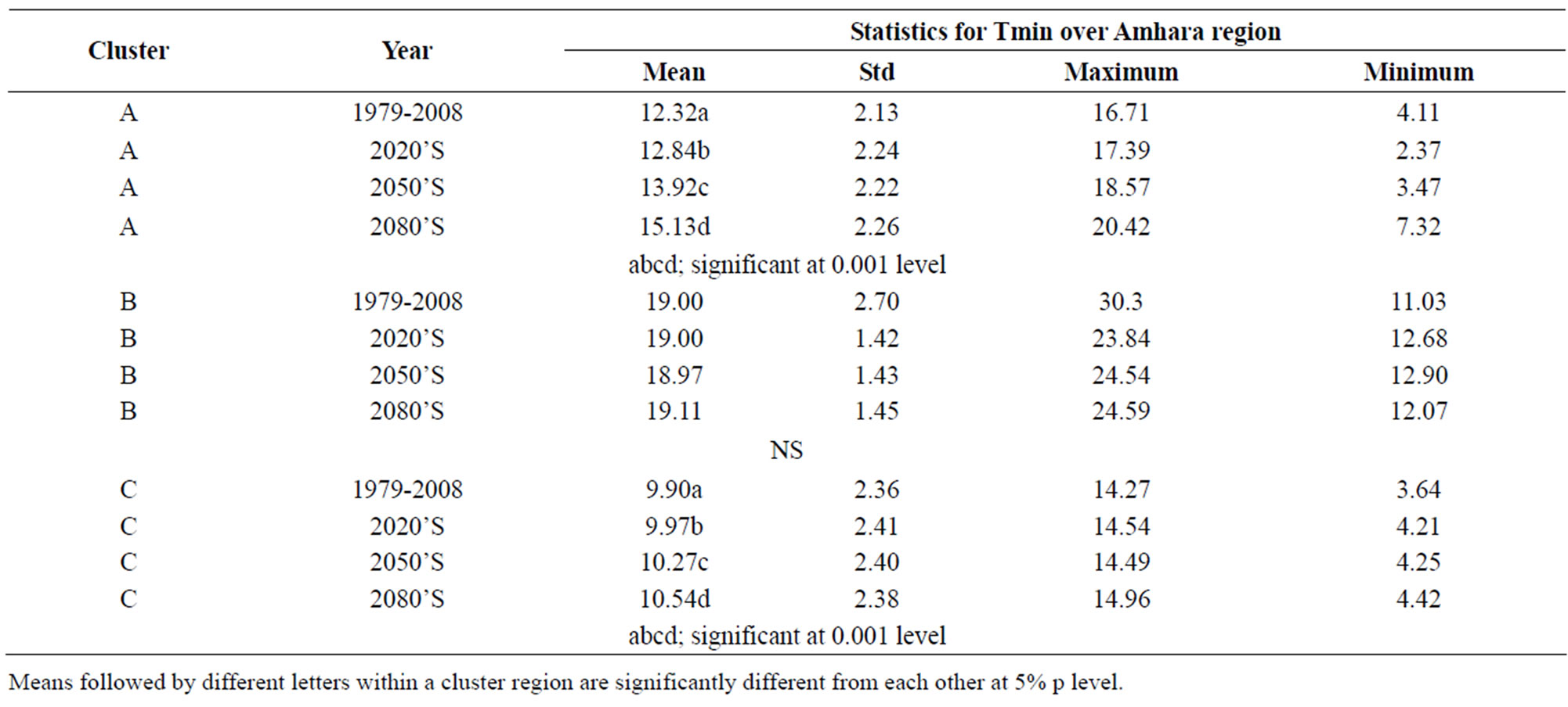
Table 7. Summered statistics mean of minimum temperature in three cluster regions in Amhara Regional State.
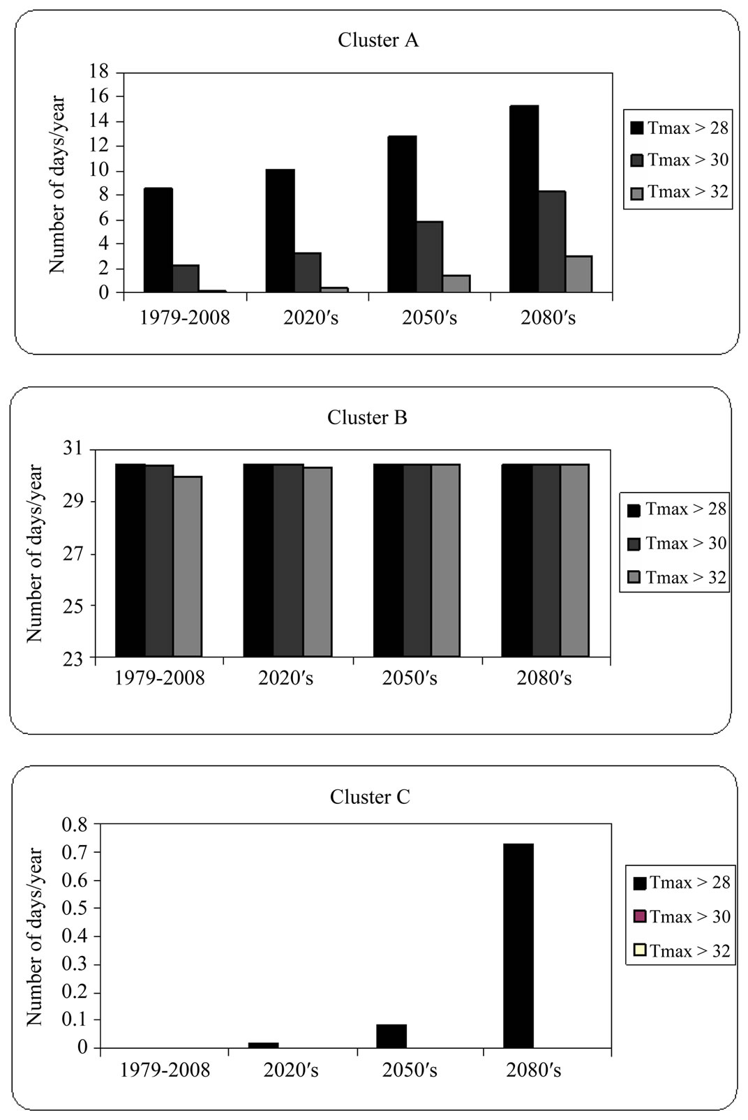
Figure 8. Projected number of hot days per year in three cluster regions in Amhara Regional State.
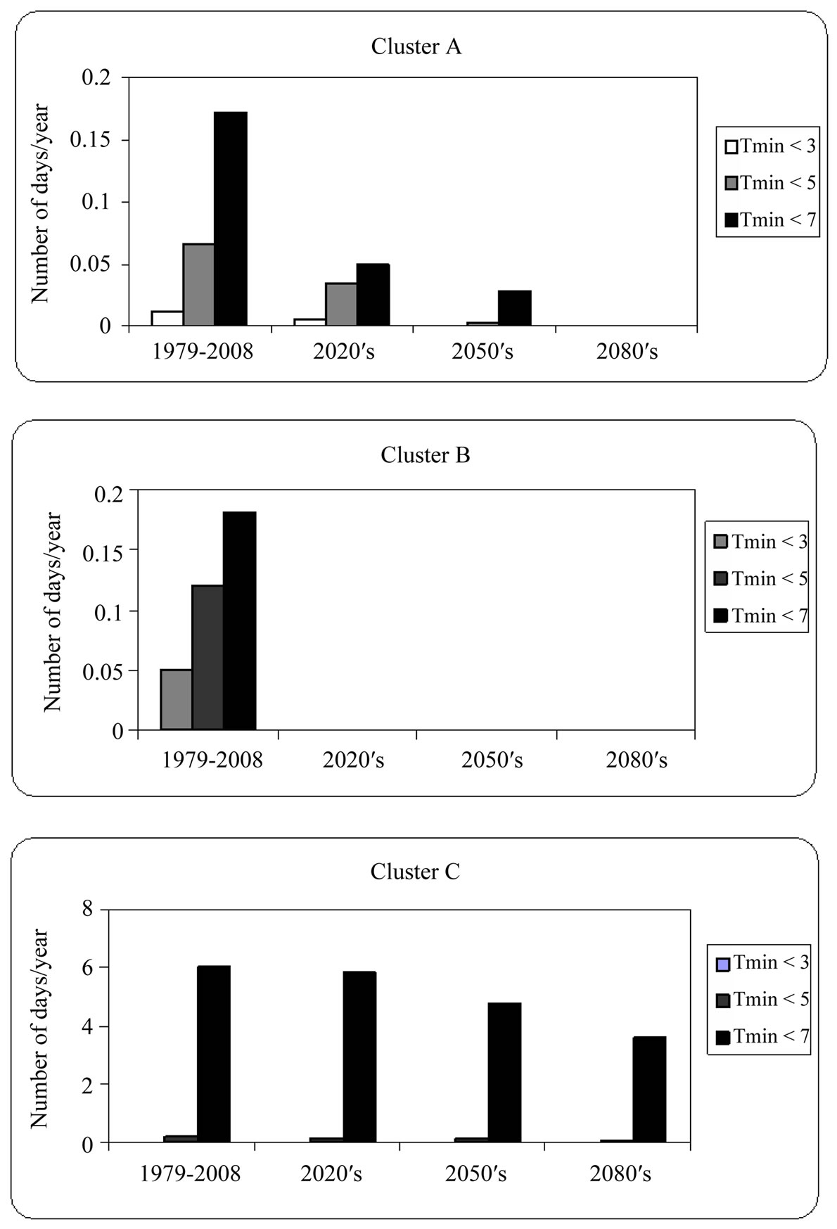
Figure 9. Projected number of cold days per year in three cluster regions in Amhara Regional State.
temperature over Ethiopia with decreasing the number of days with minimum temperature in the future.
5.7.3. Rainfall Variability and Extremesin Future Daily Pcpn
Rainfall is not usually well approximated by normal distributions [5]. The projected scenario in the current study in all clusters in the study region showed that there was a decrease in the number of positive anomalies and an increased of negative anomalies compared with the base period (1979-2008). In the base period climate, there were 13, 15 and 17 positive anomalies and 15, 15 and 13 negative anomalies in Clusters A, B and C, respectivelly As compared to 12, 10 and 13 “positive” anomalies and 14, 18 and 17 negative anomalies respectively in the 2080s (Figure 10).
This decrease in positive anomaly and increase in negative anomaly lead to an extended periods of below average rainfall in the study areas. Rainfall variability in general and decrease in positive anomalies in particular is in accordance with the decrease in projected annual rainfall by 27.2%, 42.3% and 12.2% in 2080s in cluster A, B and C, respectively (Table 5). [36] also indicated that Ethiopia’s average annual rainfall has shown a very high level of variability. Further, a study to analyze farmers’ perceptions of climate change in the Nile Basin of Ethiopia by [38] indicated that temperature has increased and the level of rainfall has declined. Furthermore, [5, 39,40], add that the climate change induced warming of the Indian Ocean is likely to lead to persistent droughts in east Africa in the coming years; hence the monsoon winds that bring seasonal rain to sub-Saharan African could be 10% - 20% drier than the 1950-2000 averages.
Similarly, the finding in this study showed the more
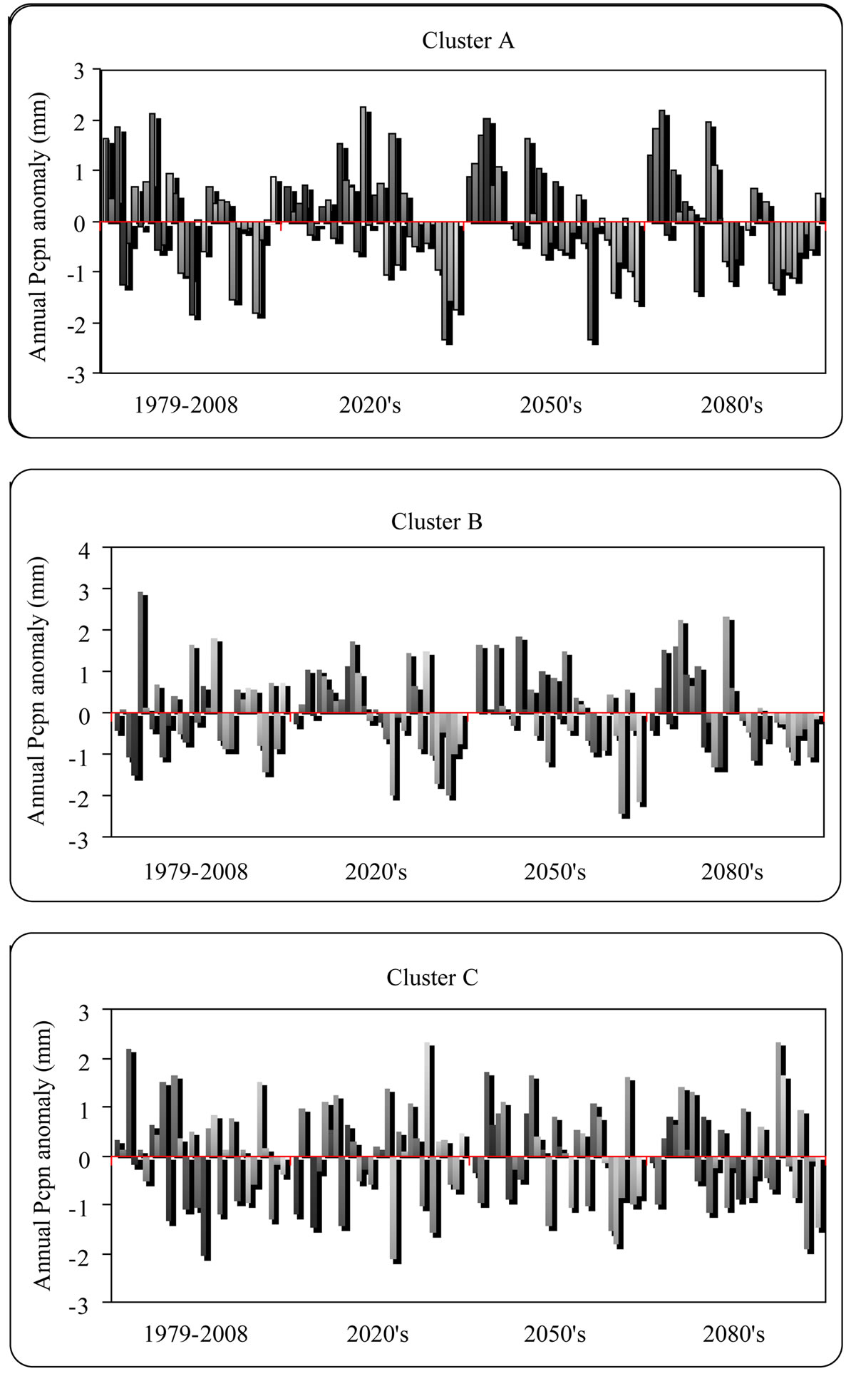
Figure 10. Annual rainfall anomaly for the period (1979-2008), 2020s, 2050s and 2080s in three cluster regions in the Amhara regional state.
likely occurrence of persistent drought, (anomalies of ≥−0.84. It means that the number of rainy days per year in future climate will decreased dramatically (Figure 10); which could shrink household farm production by up to 90 percent of a normal year output [41].
As shown in Table 5, there was high decrease in percentage change of rainfall in all clustered regions. This could be due to a dramatic decrease in the number of rainy days in the 2080s as compared to the base period (Figures 11 and 12). This finding is in agreement with the finding of [42] who noted an increase in the frequency of drought occurrence in the past few dacades in Ethiopia.
Although the annual rainfall amount decreases (Figure 12), the number of rainy days in the projected time periods at Cluster B did not decrease in equal magnitude as Clusters A and C (Figure 11).
6. CONCLUSIONS AND RECOMMENDATIONS
6.1. Conclusions
Downscaled temperature results for the Amhara region using both A2a emission scenario showed increasing
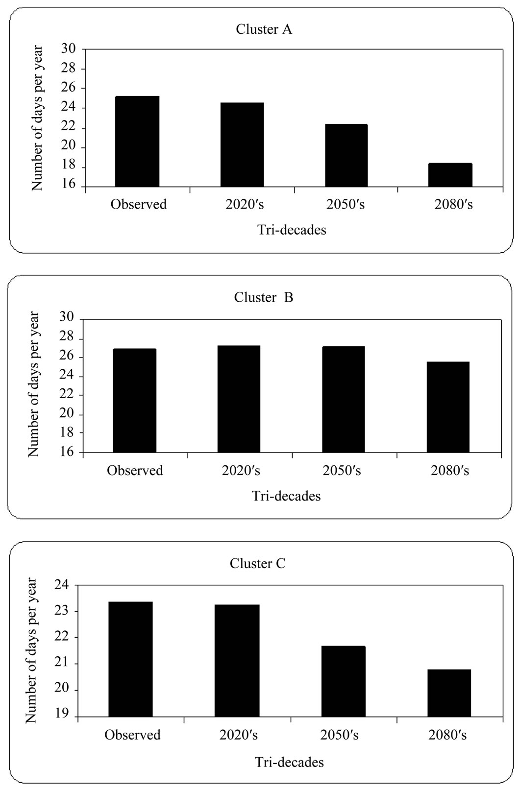
Figure 11. Projected number of rainy days per year in three cluster regions in the Amhara Regional State.
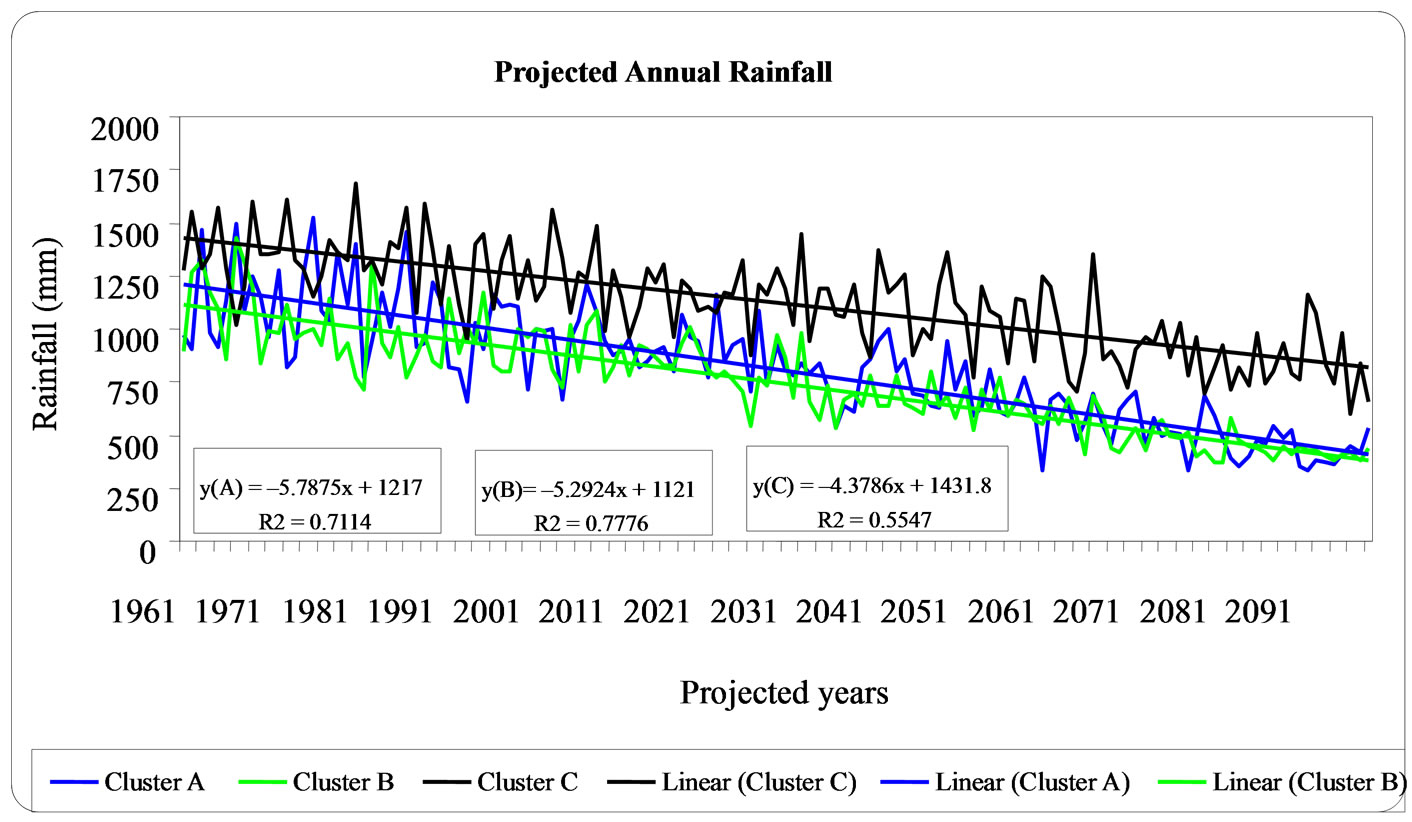
Figure 12. Future trends of rainfall in Clusters A, B and C in three cluster regions in the Amhara Regional State.
trend for the three tri-decadal periods centered on the 2020s, 2050s, and the 2080s. Maximum temperature could rise up by 2.3˚C, 4.6˚C and 1.80˚C, while minimum temperature increased by 3.6˚C, 0.3˚C and 0.50˚C in Clusters A, B and C, respectively in 2080s. Unlike temperature, rainfall results showed decreasing trend in all projected years. A percentage decrease in rainfall of about 27.2%, 42.3% and 12.2% was noted in Clusters A, B and C, respectively in the 2080s.
Generally, the effects of global warming due to greenhouse gas emissions and sea surface warming is reflected in the study area with an increase in projected temperatures and a decrease in rainfall which resulted in increased number of projected hot days, fewer number of projected cold days and decreased number of projected rainydays. These events may lead to increased occurrence of drought and water shortage over the Amhara Regional State.
6.2. Recommendations
Generally, based on the results of this study the following recommendations are forwarded: The projected changes in temperature and rainfall in the Amhara region urges decision makers to incorporate climate change scenarios in devising sustainable regional coping strategies, including: water harvesting technologies, supplementary irrigation, improved seeds which can tolerate moisture and temperature stresses, afforestations and soil conservation techniques, preventing free grazing and related strategies and measures.
The result of any model depends on the quality of the input data; therefore, to make the evaluation of climate change studies more complete, it is recommended to conduct similar studies with large number of meteorological stations and GCM models.
7. ACKNOWLEDGEMENTS
We express our sincere thanks to the Ministry of Education and Haramaya University for their financial support to carry out this work. We also express our sincere thanks to Bahir Dar University for allowing the first author to pursue his PhD study. Equally important was the support given by the Swiss NCCR North-South program and linking this particular research with the global climate implications. The National Meteorological Agency is also acknowledged for providing most of the daily rainfall and temperature data used for the study.
REFERENCES
- Gitay, H., Suarez, A., Watson, R.T. and Dokken, D.J. (2002) Climate change and biodiversity. IPCC (Intergovernmental Panel on Climate Change) technical paper V, 86. http://www.ipcc.ch
- UNEP (United Nations Environment Programme) and CMS (Convention on the Conservation of Migratory Species of Wild Animals) (2006) Migratory species and climate change: impacts of a changing environment on wild animals UNEP/CMS Secretariat, Bonn, Germany.
- The nature conservancy website. http://www.nature.org/climatechange/
- World Wide Fund for Nature (2006) Climate change impacts on East Africa: a review of the scientific literature, Gland. WWF, Morges.
- IPCC Technical Summary (2001) Climate change 2001: The dcientific basis. In: Houghton, J.T., Ding, Y., Griggs, D.J., Noguer, M., van der Linden, P.J., Dai, X., Maskell, K. and Johnson, C.A., eds., Technical Summary of the Working Group I Report, Cambridge University Press, Cambridge, 94.
- Biodiversity Strategy and Action plan (2005) Biodiversity Strategy and Action plan. BSAP. Final document.
- Davidson, O., Halsnaes, K., Huq, S., Kok, M., Metz, B., Sokona, Y. and Verhagen, J. (2003) The development and climate nexus: the case of sub-Saharan Africa. Climate Policy, 3, S97-S113. doi:10.1016/j.clipol.2003.10.007
- Zhou, G., Minakawa, N., Githeko, A.K. and Yan G. (2004) Association between climate variability and malaria epidemics in the East African highlands. Proceedings of the National Academy of Sciences of the United States of America, 101, 2375-2380.
- Craig, M.H., Kleinschmidt, I., Nawn, J.B., Le Sueur D. and Sharp, B.L. (2004) Exploring 30 years of malaria case data in KwaZulu-Natal, South Africa: part I. The impact of climatic factors. Tropical Medicine and International Health, 9, 1247-1257.
- Wood, A. (1977) A preliminary chronology of Ethiopian droughts. In: Dalby, D., Church, R.J.H. and Bezzaz, F., eds., Drought in Africa, Vol. 2, International African Institute, London, 68-73.
- Pankhurst, R. and Johnson, D.H. (1988) The great drought and famine of 1888-92 in northeast Africa. In: Johnson, D.H. and Anderson, D.M., eds., the Ecology of Survival: Case Studies from Northeast African History, Lester Crook Academic Publishing, London, 47-72.
- NOAA (The National Oceanic and Atmospheric Administration) research website. http://www.research.noaa.gov/climate/t_prediction.html
- Australian Bureau of Meteorology. http://www.bom.gov.au/analclim.htm
- Wilby, R.L. and Dawson, C.W. (2007) SDSM—A decision support tool for the assessment of regional climate change impacts. Environmental Modeling Software, 17, 145-157. doi:10.1016/S1364-8152(01)00060-3
- Wilby, R.L., Dawson, C.W. and Barrow, E.M. (2002) Statistical downscaling model SDSM, version 4.1. Department of Geography, Lancaster University, Lancaster.
- Wilby, R.L. and Dawson, C.W. (2004) Using SDSM version 3.1—A decision support tool for the assessment of regional climate change impacts. User Manual, Leicester.
- Dibike, Y.B. and Coulibaly, P. (2005) Downscaling precipitation and temperature with temporal neural networks. Department of Civil Engineering, and School of Geography and Geology, McMaster University, Hamilton.
- Kilsby, C.G., Jones, P.D., et al. (2007) A daily weather generator for use in climate change studies. Environmental Modelling and Software, 22, 1705-1719. doi:10.1016/j.envsoft.2007.02.005
- Pryor, S.C., Schoof, J.T. and Barthelmie, R.J. (2005) Empirical downscaling of wind speed probability distributions. Journal of Geophysical Research, 110, Article ID: D19109. doi:10.1029/2005JD005899
- Gordon, C., Cooper, C., Senior, C.A., Banks, H.T., Gregory, J.M., Johns, T.C., Mitchell, J.F.B. and Wood, A. (2000) The simulation of SST, sea ice extents and ocean heat transports in a version of the Hadley Centre coupled model without flux adjustments. Climate Dynamics, 16, 147-168. doi:10.1007/s003820050010
- Pope, V.D., Gallani, M.L., Rowntree, P.R. and Stratton, R.A. (2000) The impact of new physical parameterizations in the Hadley Centre climate model—HadAM3. Climate Dynamics, 16, 123-146. doi:10.1007/s003820050009
- Reichler, T. and Kim, J. (2008) How well do coupled models simulate today’s climate? Bulletin of the American Meteorological Society, 89, 303-311. doi:10.1175/BAMS-89-3-303
- Souvignet, M. and Heinrich J. (2008) Future temperatures and precipitations in the arid northern-central Chile: A multi-model downscaling approach. 6th Alexander von Humboldt International Conference, 24 June 2010.
- Zeray, L., Roehrig, J. and Alamirew, D. (2006) Climate change impact on Lake Ziway watershed water availability, Ethiopia. Conference on International Agricultural Research for Development, Tropentag, 11-13 October 2006.
- Tachieobeng, E., Gyasi, E., Abekoe, S.A.M. and Ziervogel, G. (2010) Farmers’ adaptation measures in scenarios of climate change for maize production in semi-arid zones of Ghana. 2nd International Conference on climate, sustainability and development in Semi-arid Regions, Fortaleza, 16-20 August 2010.
- Central Statistics Authority (2005) The federal democratic Republic of Ethiopia statistical abstract. CSA, Addis Ababa.
- Federal Democratic Republic of Ethiopia (1997) The conservation strategy of Ethiopia: The resources base, its utilization and planning for sustainability, vol. I. Environmental protection authority in collaboration with the ministry of economic development and cooperation. FDRE, Addis Ababa.
- Intergovernmental Panel on Climate Change (2011) the IPCC Data Distribution Center. http://www.ipcc-data.org/
- Canadian Institute for Climate Studies (CICS). http://www.cics.uvic.ca/scenarios/sdsm/select.cgi
- Houghton, J.T. (2001) Climate change the scientific basis: contribution of working group I to the third assessment report of the intergovernmental panel on climate change. Cambridge University Press, Cambridge.
- Robert A. and Wither P. (2007) StatistiXL, version 1.8, a powerful statistics and statistical analysis add-in for Microsoft Excel. Microsoft, Washington DC.
- Stern, R., Knock, J., Rijks, D. and Dale, I. (2002) Instat+ (interactive statistics package). Statistics services center. University of Reading, Reading.
- National Meteorological Services Agency (1985) Climate and agro climatic resources of Ethiopia. Addis Ababa.
- Francis, D. and Hengeveld, H. (1998) Extreme weather and climate change. http://www.mscsmc.ec.gc.ca/education/scienceofclimatechange/understanding/ccd/ccd_9801/sections/1_e.html
- NCAR (National Centre for Atmospheric Research) (2005) A continent split by climate change: New study projects drought in southern Africa. Boulder Co., Nairobi.
- National Meteorological Services (2007) Climate change national adaptation program of action (NAPA) of Ethiopia. NMS, Addis Ababa.
- National Meteorological Services Agency (2001) Initial national communication of Ethiopia to the United Nations framework convention on climate change (UNFCCC). NMSA, Addis Ababa.
- Temesgen, D. (2007) Measuring the economic impact of climate change on Ethiopian agriculture: Ricardian approach. World Bank policy research paper No. 4342. World Bank, Washington DC.
- Hulme, M., Doherty, R., Ngara, T., New, M. and Lister, D. (2001) Taking action against climate change in Ethiopia and South Africa.
- Funk, C., Senay, G., Asfaw, A., Verdin, J., Rowland, J., Michaelson, J., Eilerts, G., Korecha, D. and Choularton, R. (2005) Recent drought tendencies in Ethiopia and equatorial-subtropical eastern Africa. FEWS-NET, Washington DC.
- World Bank (2003) Risk and vulnerability assessment draft report. World Bank, Addis Ababa.
- Ketema, T. (1999) Test of homogeneity, frequency analysis of rainfall data and estimate of drought probabilities in dire Dawa, eastern Ethiopia. Ethiopian Journal of Natural Resources, 1, 125-136.
NOTES
#Current address: International Maize and Wheat Improvement Center (CIMMYT), Addis Ababa, Ethiopia.