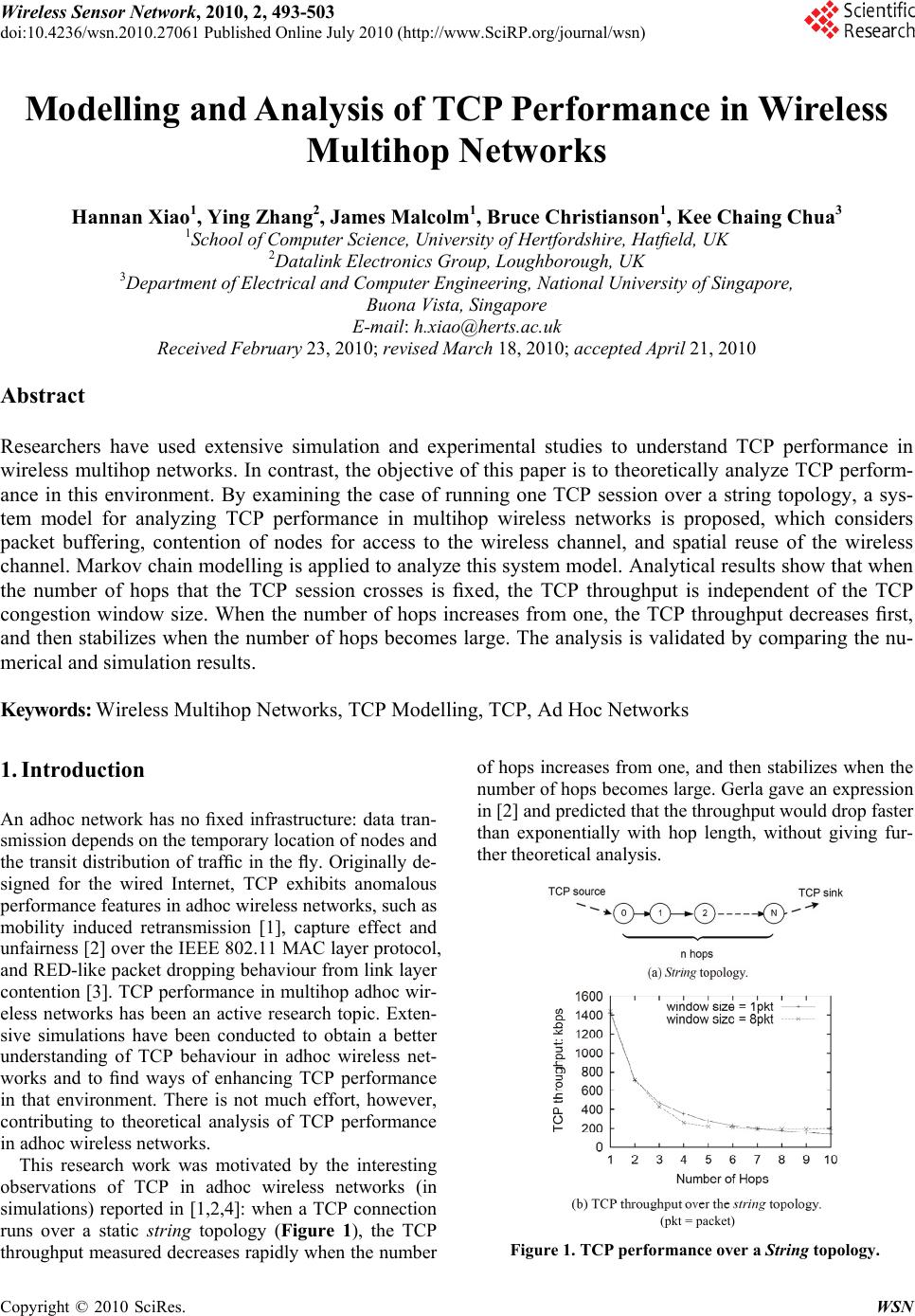Wireless Sensor Network, 2010, 2, 493-503
doi:10.4236/wsn.2010.27061 Published Online July 2010 (http://www.SciRP.org/journal/wsn)
Modelling and Analysis of TCP Performance in Wireless
Multihop Networks
Hannan Xiao1, Ying Zhang2, James Malcolm1, Bruce Christianson1, Kee Chaing Chua3
1School of Computer Science, University of Hertfordshire, Hatfield, UK
2Datalink Electronics Group, Loughborough, UK
3Department of Electrical and Computer Engineering, National University of Singapore,
Buona Vista, Singapore
Received February 23, 2010; revised March 18, 2010; accepted April 21, 2010
Abstract
Researchers have used extensive simulation and experimental studies to understand TCP performance in
wireless multihop networks. In contrast, the objective of this paper is to theoretically analyze TCP perform-
ance in this environment. By examining the case of running one TCP session over a string topology, a sys-
tem model for analyzing TCP performance in multihop wireless networks is proposed, which considers
packet buffering, contention of nodes for access to the wireless channel, and spatial reuse of the wireless
channel. Markov chain modelling is applied to analyze this system model. Analytical results show that when
the number of hops that the TCP session crosses is fixed, the TCP throughput is independent of the TCP
congestion window size. When the number of hops increases from one, the TCP throughput decreases first,
and then stabilizes when the number of hops becomes large. The analysis is validated by comparing the nu-
merical and simulation results.
Keywords: Wireless Multihop Networks, TCP Modelling, TCP, Ad Hoc Networks
1. Introduction
An adhoc network has no fixed infrastructure: data tran-
smission depends on the temporary location of nodes and
the transit distribution of traffic in the fly. Originally de-
signed for the wired Internet, TCP exhibits anomalous
performance features in adhoc wireless networks, such as
mobility induced retransmission [1], capture effect and
unfairness [2] over the IEEE 802.11 MAC layer protocol,
and RED-like packet dropping behaviour from link layer
contention [3]. TCP performance in multihop adhoc wir-
eless networks has been an active research topic. Exten-
sive simulations have been conducted to obtain a better
understanding of TCP behaviour in adhoc wireless net-
works and to find ways of enhancing TCP performance
in that environment. There is not much effort, however,
contributing to theoretical analysis of TCP performance
in adhoc wireless networks.
This research work was motivated by the interesting
observations of TCP in adhoc wireless networks (in
simulations) reported in [1,2,4]: when a TCP connection
runs over a static string topology (Figure 1), the TCP
throughput measured decreases rapidly when the number
of hops increases from one, and then stabilizes when the
number of hops becomes large. Gerla gave an expression
in [2] and predicted that the throughput would drop faster
than exponentially with hop length, without giving fur-
ther theoretical analysis.
(pkt = packet)
Figure 1. TCP performance over a String topology.

H. N. XIAO ET AL.
494
In this paper, a system model for analyzing TCP per-
formance in adhoc wireless networks is proposed after
examining the case of running one TCP session over a
string topology. The system model considers the features
of wireless multihop network such as contention of
nodes for access to the wireless channel, packet buffering
intermediate nodes, and spatial reuse of the wireless
channel. A Markov chain modelling is applied to analyze
this system model starting from a single hop case to mul-
tiple hop cases. Analytical results show that when the
number of hops that the TCP session crosses is fixed, the
TCP throughput is independent of the TCP congestion
window size. When the number of hops increases from
one, the TCP throughput decreases first, and then stabi-
lizes when the number of hops becomes large. The
analysis is validated by comparing the numerical and
simulation results.
The rest of the paper is organized as follows. Section 2
discusses related work in two areas, i.e., TCP perform-
ance in multihop wireless networks and system models
for TCP analysis in different networks. Section 3 pro-
poses a system model for analyzing TCP performance in
multihop wireless networks, following which Section 4
applies a Markov chain modelling of the system model.
Section 5 presents the theoretical analysis of the TCP
throughput over the string topology from specific cases
to the general case and Section 6 evaluates the analysis
by comparing the simulation and numerical results. Fi-
nally Section 7 concludes the paper.
2. Related Work
2.1. TCP Performance in Wireless Multihop
Networks
TCP was initially designed for wired networks to provide
reliable data transmission by retransmitting lost packets
due to network congestion that is detected at the sender
by time-out or duplicated acknowledgments. Packet loss
triggers TCP congestion control which reduces the cong-
estion window size, effectively the sending rate, as a
reaction to network congestion. TCP, however, has per-
formed poorly in wireless multihop networks where
packet loss may happen from various reasons other than
network congestion, such as error-prone wireless link,
link layer contention and routing failure or breakage.
Many approaches have been proposed to improve TCP
performance in the environment of wireless multihop
networks from different aspects. Based on the nature of
the approaches, they may be summarized into three
groups as in [5]:
 TCP with feedback [1,6-11] where feedbacks from
networks are sent back to the sender to distinguish
packet losses due to congestion from link error,
link contention or routing breakage or failure.
 TCP without feedback [12,13] where TCP conges-
tion control strategy is modified according to the
scenarios in multihop wireless networks.
 TCP with lower layer enhancement [14-18]. This
approach is more popular recently as more work
have been done to understand the cross-layer in-
teraction, especially lower layer impact on TCP
performance in wireless multihop networks.
The above work shares one similarity i.e., they all ob-
serve TCP performance in multihop wireless networks
by simulations and then propose improvements. Very
few works, however, have been devoted on theoretical
analysis of TCP performance in multihop wireless net-
works. We proposed a system model for TCP analysis
over one-hop string topology as early as in 2001 [19] and
then extended the modelling to multihop cases in [20].
So far our analysis only applies when there is no packet
loss in the multihop wireless TCP packet transmissions.
Multiple lossy links are modelled in [21] which also
consider different proportions between the interference
range and transmission range in the spatial reuse prop-
erty of the wireless channel.
2.2. System Models for TCP Analysis
There are various approaches to modelling TCP in the
literature. Some papers have tried to capture the essential
TCP dynamics through closed-form expressions. Lak-
shman and Madhow [22] and Kumar [23] use Markovian
analysis to develop a closed-form expression for the thr-
oughput of TCP connections by observing the cyclical
evolution of the TCP transmission window. The latter
work introduces some extensions for several versions of
TCP, incorporating such features as coarse timers, fast
retransmit and fast recovery. Mathis et al. [24] focus on
the stochastic behavior of the congestion avoidance
mechanism, deriving an expression for the throughput
that is then applied to study the behavior of several
flavors of TCP sources and queueing techniques. Padhye
et al. [25] have derived a steady-state model that ap-
proximates the throughput of bulk TCP flows as a func-
tion of loss rate and round trip time, comparing their es-
timates with real-life traces of TCP traffic. In [26], in-
stead of trying to establish a closed-form expression for
key metrics such as throughput, queueing delay and
packet loss, a novel methodology, reciprocal model tun-
ing, combines a Markovian model of a single TCP sou-
rce in isolation, and the analysis of superposition and
interaction of several TCP sources through standard
queueing analysis techniques. Notably, some researchers
[27,28] have chosen a different approach whereby the
observation of “actual” TCP traces is the foundation of
empirical models. These efforts imply collecting hours’
(days’) worth of data, and finding suitable statistical dis-
tributions for the observed data.

H. N. XIAO ET AL.
495
There are two system models in the literature most
similar to our model. The first one is used by Chaskar,
Lakshman and Madhow in [29] to analyze TCP per-
formance over a wireless channel with link level error
control. There, ACK packets are assumed to arrive in the
source node after a constant delay and are never lost.
Thus the path of ACKs is omitted (Figure 2(a)). The
second one is proposed by Lakshman, Madhow and
Suter in the same research group to analyze TCP per-
formance with random loss and bidirectional congestion
[30]. There, for the first time the path followed by ACKs
is explicitly modeled (Figure 2(b)). These models, how-
ever, cannot be used in our case of multihop wireless
networks where the TCP packets and ACKs are con-
tented to use the same wireless channel. Instead of start-
ing with analyzing the TCP protocol with assumptions as
in [22-26], our approach is to study the process of how
TCP works between a source and destination pair by
examining the simulation trace file. The resulting model
considers the channel access probability of both the
source and the destination (Figure 3).
3. System Model
Consider the simple adhoc wireless network scenario
shown in Figure 1 nodes form a string with length N.
Each node has the same transmission radius, the same
carrier sense radius, and the same interference radius.
One TCP connection is run from node 0 to node N
crossing all the intermediate nodes in the string.
We model the communication process of the TCP
connection as in Figure 3 after analyzing the trace files
from simulations carefully. The source and destination
nodes both have a First In First Out (FIFO) forward
buffer of size. The source has infinite data to send, so that
TCP packets are always of the maximum packet size. For
each packet that is received by the destination, a cumula-
(a)
(b)
Figure 2. Reference system models for TCP analysis.
Figure 3. System model of TCP in wireless ad-hoc networks.
tive acknowledgment (ACK) is generated which can be
modeled as containing the next expected segment num-
ber. TCP packet service rate is t U, the typical number
of TCP packets the system serves per unit time when it is
constantly busy. ACK packet service rate is a U, the
typical number of ACK packets the system serves per
unit time when it is constantly busy. The “unit time” in-
cludes TCP/ACK packet transmission delay, propagation
delays, processing delays at the nodes from layer to layer
and the average MAC layer contention delays. The
TCP/ACK packet service rates are affected by the spatial
reuse of wireless channel in the string topology. As all
nodes compete to use the channel, the chance for any
node to send packet is determined by the underlying
MAC protocol and traffic distribution. Generally, we
denote the average probability of the source to send a
TCP packet as q, and the average probability of the
destination to send an ACK packet as p. The reason to
use the average probability of the node accessing the
channel is because the performance metric of interest is
the average TCP throughput.
The system model captures the unique communication
features of TCP in adhoc wireless networks including
link layer channel contention and channel spatial reuse. It
is similar to but different from system models used in
analyzing TCP performance in other kind of networks
[29,30].
4. Markov Chain Modelling
We use Markov chain modelling to analyze the proposed
system model. Firstly, a discrete Markov chain is formed
for the case when the source and the destination are sin-
gle-hop away. The Markov chain is then extended to the
general case when the source and the destination are
multiple hops away. The assumptions made are as fol-
lows:
 There is no random loss of packets due to channel
error. The channel appears error-free to the upper
layer because of the error coding schemes and link
layer retransmission protocols.

H. N. XIAO ET AL.
496
 The channel also appears collision-free to the up-
per layer because the MAC layer protocol is colli-
sion avoided, such as MACAW [31].
 The maximum TCP congestion window size is less
than the buffer size at each node.
 There is no packet dropping due to buffer overflow,
and no packet loss due to link layer contention.
This assumption is supported by simulation results
demonstrating that packet loss due to buffer over-
flow is rare and packet loss due to link contention
is very low for single TCP over a string topology.
 The distribution of inter-service time of TCP pac-
kets and ACK packets are exponentially distrib-
uted which include packet retransmissions. This
assumption is based on the fact that exponential
backoff during contention is commonly used in
MAC protocols, e.g., IEEE 802.11.
4.1. Single-Hop Case
There are only TCP packets at the source and only ACK
packets at the destination. Either the source or the desti-
nation sending packets will change the number of the
packets queued in their buffers. Ignoring the slow start
phase which is a small part of the data transmission, the
sum of the TCP packets at the source and the ACK pack-
ets at the destination equals to the TCP congestion win-
dow size in packets. As it is assumed that no packet loss
exists due to channel error, buffer overflow, or link con-
tention, the TCP connection thus increases its congestion
window size to the maximum value and stabilizes there.
Discrete-time Markov chain is applied to analyze TCP
performance here. Let us focus attention at times 0,

,

2…,

k,… as in [32] (pages 162-173), where

is
a small positive number. Let
F
denote as the number of
TCP packets in the source node buffer at time

k.
F
thus is a Markov chain on the state-space {Wm :
0m}, where W the maximum TCP congestion win-
dow size. The transition diagram of the Markov chain is
shown in Figure 4.
When there are WTCP packets in the source node,
i.e., the first state in Figure 4, the destination node does
not have ACK packets to send. Therefore, the source
node catches the wireless channel for sure. The resulting
transition probability from the state of WF  to

F
1

W is t U

, where t U is the service rate of TCP
packets and the inter-service time is assumed to be ex-
ponentially distributed. Similarly, the transition probabil-
ity from the state of 0

F to 1
F
is a U

Where
a
U is the service rate of ACK packets and the inter-
service time is assumed to be exponentially distributed.
When there are F, where 11WF  TCP packets
in the source, there are FW

ACK packets in the des-
tination node. The source node and destination node
compete with each other to use the channel. The source
node has average probability of q to access the channel
(Figure 3), the transition probability from the state of
iWF


to 1



iWF is thus t Uq

, where
11



Wi . Similarly, the transition probability from
the state of iWF


to 1 iWF is a Up

, where
p is the average probability of the destination to access
the channel.
4.2. Multiple-Hop Case
When the source and destination are multiple hops away,
an accurate Markov model at times

kwould be on the
state space )},(),...,,(),,{(1100 NN AFAFAF , where ),( iiAF
are the numbers of TCP and ACK packets at node i.
This multi-dimensional Markov chain modelling consid-
ers the number of TCP packets and ACK packets in the
source, the destination and the intermediate nodes along
the string topology. Unfortunately, such a modelling is
difficult to tackle. For example, even when the string
topology is 2-hops long, and the TCP maximum conges-
tion window size is 2 packets, the Markov chain already
has 11 states as shown in Figure 5, and the number of
states increases quickly with the increase of the TCP
maximum congestion window size and the length of the
string. This happens due to the sharing of wireless chan-
nel between nodes. When two nodes within interference
range both have packets to send, there are two possible
next states. The more states the Markov chain has, the
more difficult it is to solve. A heuristic alternative is ap-
plied as follows.
The more states the Markov chain has, the more paths
are available in the transition diagram for a TCP packet
1000
100
01 00
000 1
0000 1
t t
aa tt
aa tt
aatt
a a
UU
pUpU qUqU
pUpU qUqU
Q
pUpU qUqU
UU






 
 

 
 

 
 
 

 

 
 






(1)

H. N. XIAO ET AL.
497
11111
Figure 4. Transition diagram when the number of hop is 1 and TCP maximum congestion window size is W.
Figure 5. Transition diagram when the number of hop is 2
and the maximum TCP congestion window size is 2 packets.
The number of TCP packets at nodes are shown as 1 or 2;
the number of ACK packets are shown as 1’ or 2’. (1, 1’, 0)
denotes that there is 1 TCP packet at the source node, 1
ACK packet at the middle node, and none packet at the
destination node.
to be transmitted from the source to the destination, or
for an ACK packet from the destination to the source.
Whatever states the packet goes through in between, it
finally passes all the nodes of the string. Let us denote
the path for a TCP packet to be transmitted from the
source to the destination as a forward path; and the path
for an ACK packet to be transmitted from the destination
to the source as a backward path. A transmission round
of TCP is composed of one forward path and one back-
ward path.
The average utilization of the string topology should
be the average of all the transmission rounds. Intuitively,
for each forward path, a corresponding complementary
backward path exists which makes this round of trans-
mission to be exactly the average value. With this un-
derstanding, the analysis can be sought out based on a
specific transmission round with a pair of complemen-
tary forward and backward paths only. All the TCP
packets go through the specific forward path, and all the
ACK packets go through the specific backward path in
such analysis.
A simple transmission round is chosen as follows: for
the forward path, when the source node gets chance to
start sending a TCP packet, the packet passes all the in-
termediate nodes continuously until it reaches the desti-
nation; the forward path can be path 1 or path 2 in Fig-
ure 5. Likewise, for the backward path, when the desti-
nation node gets chance to start sending an ACK packet,
the ACK packet passes all the intermediate nodes con-
tinuously until it reaches the source; the backward path
can be path 3 or path 4 in Figure 5. These paths are
complementary.
In the above specific transmission round, once one pa-
cket in the source node is sent out, the number of packets
in the buffer of source node decreases by 1. After the
packet goes continuously to the destination, the destina-
tion absorbs the TCP packet and generates an ACK
packet. The reverse process is the same. Consequently,
the changing of number of packets in the source and the
destination is the same as in the single-hop scenario. The
Markov modelling of this complete transmission round is
thus exactly the same as in Figure 4 when we only con-
sider the marked paths and states in Figure 5.
In the following subsections, we are going to analyze
the discrete Markov chain in Figure 4 for both the sing-
le-hop and multiple-hop cases.
5. Analysis
5.1. TCP Throughput
The transition matrix Qof the Markov chain in Figure
4 is listed in (1). Let ww1 0 (,,...)πππ π

denote the
stationary probability distribution of the Markov chain,
we have Q




at steady state. From this it is derived
that
2
w1 w
w2 w
ww
0w
1
1
1, 11
i
i
w
q
qp
q
qp
qiW
qp
pq
qp















 







(2)
where

is the ratio of t U to a U, i.e.,
a
t
U
U
 
.
From 1
0

W
ii
 , it is further derived that
w1
1
1
1
1()()
WiW
i
qpq
qp qp







 (3)

H. N. XIAO ET AL.
498
From the transition diagram, we denote the TCP
throughput of state i by i

and the average through-
put of TCP packets by

. Thus  W
iii 0
 , where
,
wti t
UqU

  when 11  iW , and 0
0


. The-
refore,
1( )
1
w
tw
q
p
Uq
p






(4)
The source and destination nodes are located at the
two ends of the string topology with 1N intervening
nodes. The positions of the source and destination are the
same, and they also have the same number of packets to
send since we assume that one ACK is generated for
each TCP packet. Thus, the source and destination nodes
have the same average probability to access the channel
successfully, i.e., qp. (3) and (4) can then be simpli-
fied as:
11
1
1
1(1)(1)
w
WW
q







(5)
)1()1
1
()1(
1
11 


WW
W
t
q
U



(6)

is the ratio of TCP packet service rate to the ACK
packet service rate. Since TCP packets and ACK packets
are transmitted at the same channel, and they travel the
same number of hops between the source and the desti-
nation,

is always approximately equal to the ratio of
the TCP packet service rate to the ACK packet service
rate in the case when there is only one hop between the
source and the destination. This is further approximately
equal to the ratio of the ACK packet size to the TCP
packet size. The TCP packet (say, 1460 bytes) is nor-
mally much larger than the ACK packet (say 40 bytes),

is thus much smaller than 1 (say, around 40/1460 =
0.027), i.e., 1

. The maximum TCP congestion
window size W pkts is an integer and when it is big
enough, it is expected that
11 111 WWW
 (7)
Thus from (6) and (7), the average TCP throughput is
derived as:


)1
1
(1
1


q
Ut (8)
In the above analysis, it is shown clearly that the ratio
of ACK packet size to TCP packet size being much less
than 1 is required to carry out the approximation.
5.2. TCP Service Rate
We have defined t U as the service rate of TCP packets
seen q as the average probability for the source node to
access the wireless channel. Their values, however,
change with the length of the string, i.e. , the number of
hops that the TCP session crosses from the source to the
destination (Figure 1). This is because of the effect of
global channel spatial reuse and local channel contention
in adhoc wireless networks. By definition, service rate is
the “typical number of customers the system serves per
unit time when it is constantly busy” [32] (page 152).
When the number of hops is N, let the average number
of TCP packets being transmitted (served) in the system
be N
I and the service time to transmit a packet be N T,
the definition of service rate gives:
N
N
tN T
I
U (9)
Let
N
q be the average probability that the source
node accesses the wireless channel when the number of
hops is N. As N changes, N
I, N T, and
N
qalso
change. In the following, we evaluate the values of N I,
N
T, and
N
qas N changes.
5.2.1.
N
is 1, 2, 3 or 4
When N is 1, 1
1Ipkt, 2
1
1q. Let TT  1, where
T is the service time to transmit a packet over one hop
when the source and destination nodes are one hop away.
When N is 2, each TCP packet travels two wireless
links to reach the destination. Therefore, approximately
TT 2
2

. During the transmission from node 0 to node 1,
and then from node 1 to node 2, only 1 TCP packet can
be transmitted in the system without collision. Therefore
pktI 1
2. In the string topology, the source node only
forwards TCP packet, the destination node only forwards
ACK packets but the middle node forwards both TCP
and ACK packets. Since one ACK packet is assumed for
each TCP packet, the middle node sends out packets
twice as much as the source and destination node. As a
result, the average probability of the middle node to ac-
cess the channel successfully is twice as much as that of
the source and destination node. In addition, the summa-
tion of the average probability of all nodes to access the
channel is 1. Derivation from these relationships gives
4
1
2q. When Nis 3, by similar analysis we have
333
1
1pkt, 3, 6 ITTq


.
When N is 4, it looks that node 0 and node 3 could

H. N. XIAO ET AL.
499
send packets concurrently without collision. However,
although node 3 is outside of node 1’s transmission range,
it is within the carrier sensing range and interference
range of node 1. Node 3 is thus a potential hidden termi-
nal of the transmission pair node 0 to node 3. Conse-
quently, only 1 TCP packet can be transmitted in the
system without collision. This analysis is consistent with
that in [3]. Further derivation gives 41 pkt,I ,4
4TT

8
1
4q.
We summarize the value for N
I,
N
qas shown in
Table 1.
5.2.2.
N
is 5, 6, 7, or 8
When N is 5, each TCP packet crosses five wireless
hops to reach the destination. Among the five hops from
node 0 to node 5, the 1st hop (i.e., from node 0 to node 1)
and the 5th hop (i.e., from node 4 to node 5) can be util-
ized at the same time as shown in Figure 6. But when
the 2nd , 3rd or 4th hop isused, only that hop can be used
without collision.
Assuming that the system is utilized fully, the number
of packets in the system is:
st th
5nd rdth
2 pktswhen the 1 and 5 hops
are used
1 pktwhen the 2 , 3 or 4 hops
are used
I







Since each hop has equal opportunity to be utilized,
the average number of packets in the system is: 2
3I
23
1 pkts
55
.
Table 1. N is 1, 2, 3 or 4
N N T N
I N
q
1 T
1 pkt 2
1
2 2T
1 pkt 4
1
3 3T
1 pkt 6
1
4 4T
1 pkt 8
1
Figure 6. Two TCP packets are transmitted together when
N = 5.
Although there are six nodes, however, node 0 com-
petes to use the channel locally with nodes 1, 2, 3 and 4
only. The probability for node 0 to access the channel
can therefore be taken as the same as when there are 4
hops. Thus 55
1, 5
8
qTT .
When N is 6, each TCP packet crosses six wireless
links to reach the destinatiopn. Figure 7 shows the sce-
narios when two of the six wireless links are utilized at
the same time. The number of packets in the system is:
st nd
th th
6
rd th
2 pktswhen the (1or 2) and
(5 or 6) hops are used
1 pktwhen the 3 or 4 hop is used
I





The average number of packets in the system is: 
6
I
42
21 pkts
66
 . It is also easy to get ,
8
1
6q TT6 6

.
Similarly, when N is 7, we get
st ndrd
th thth
7
th
2 pktswhen the (1, 2 or 3) and
(5, 6 or 7) hops are used
1 pktwhen the 4 hop is used
I





777
61 1
21 pkts, , 7
77 8
I
qTT
When N is 8, 88 2 pktsII , when the (1st, 2nd,
3rd or 4th) and (5th, 6th, 7th or 8th) hops are occupied, and
TTq 8,
8
1
88  .
5.2.3. Generalization of TCP Service Rate
Let jMN


4, where  4,3,2,1,1  jM , the
generalization of the above analysis is as follows.
When N is
M
4, we have 44
p
kts
MM
IIM .
When N is 14

M
,
Figure 7. Two TCP packets are transmitted together when
N = 6.

H. N. XIAO ET AL.
500

st th
th
nd rdth
41 th thth
th th
1 pktswhen the 1 and5 and
(41) hops are occupied
pktwhen the (2, 3 or 4) and
(67or8)and
(4M-2,(41)or
M
M
M
M
I,
M








th
(4M)) hops are occupied











41
1(41)(1)
( 1)pkts
41 41
M
MMM
IM M
M
M


 

Similar derivation gives:
When N is 24 
M
,
st nd
th th
th th
42 rd th
th th
1 pktswhen the (1 or 2) and
(5 or 6 )and and
(43) or (42)
hops are occupied
pktwhen the ( 3 or 4) and
(7or8)
M
M
MM
IM






th th
and and
(4-1) or (4)
hops are occupied
MM














42
2( 1)
(1)
42
(42) 2(1)
pkts
42
M
M
IM M
MM
MM


 

 
.
When N is 34 M,
st ndrd
th thth
th th
43 th
th
1 pktswhen the (1, 2 or 3) and
(5 , 6 or 7)and and
(43) or (42)or
(41)hops are occupied
pktswhen the 4
M
M
MM
IM
M





th
th
8and
and (4) hops are occupied
and
M












43
3( 1)
(1)
43
(43)3(1)
pkts
43
M
M
IM M
MM
MM


 
 
 
.
Finally, it is summarized that:
4
(1)(4 )(1)
( 1)pkts
44
Mj
jMMjjM
IM M
Mj Mj


 

(10)
Where
 4,3,2,1,1jM.
Combining (10) and the analysis when N is 1, 2, 3
or 4 in Table 1, we have the average number of packets
in the system as:
jM
MjMj
IjM 


4
)4()1( 22
4 (11)
Where

 4,3,2,1,0  jM .
The service time to transmit a packet is generalized as
TjMT jM



)4( 4. From (9), the TCP service rate is
derived as:
T jM
MjMj
UjMt
1
)4(
)4()1(
2
22
)4( 



 (12)
where

 4,3,2,1,0  jM .
The average probability of the source to access the
channel is:


4
1when 0 and 1,2,3,4
2
1when 1 and 1,2,3,4
8
Mj
Mj
j
q
Mj








(13)
5.3. Generalization of TCP Throughput
Substituting (12) and (13) into (8), the TCP throughput
becomes:
























4,3,2,11
1
71
1
)4(
)4()1(
4,3,2,10
1
))12(1(
1
2
22
4
j andM when
TjM
MjMj
j andM when
Tjj
jM



(14)
When
M
goes to infinity, jMN  4 goes to in-
finity, we have
4
11 1
lim 417
Mj
MT



 
 (15)
Equation (14) shows that the TCP throughput is inde-
pendent of the maximum TCP congestion window size
W; instead it is decided by (a) jM4, the value of the
number of hops of the string topology, (b)

, the ratio
of service rate of TCP packet to ACK packet, and (c) T,
the time needed for a TCP packet to be transmitted over
a single hop. Furthermore, (15) illustrates that as the
number of hops increases and goes to infinity, TCP
throughput converges to a constant value.
6. Evaluations
The analytical results are verified by the comparison of

H. N. XIAO ET AL.
501
simulation results in ns2 and numerial results in Matlab.
In simulations, 1N nodes forma string (Figure 1)
with adjacent nodes 200 m apart. All nodes communicate
with identical, half-duplex wireless radios which have a
bandwidth of 2 Mbps and a nominal transmission radius
of 250 m. Nodes have carrier sense radius of 550 m and
interference radius of 550 m. They are configured with
the Dynamic Source Routing (DSR) protocol. One TCP
Reno session is introduced from node 0 (TCP source) to
node N (TCP destination) to transfer FTP bulk data,
crossing N hops. TCP and ACK packets size are of
1460 bytes and 40 bytes respectively. Simulations were
run with various numbers of hops and various maximum
TCP congestion window sizes. One simulation with the
same number of hops and the same maximum TCP con-
gestion window size was run for five times, each for 300
secs, and the overall throughput was measured from 50
secs to 250 secs. During the time the throughput is quite
stable, but the average of five simulations was used as
the simulation result.
To get the numerical results in Matla b, two parameters
are needed:


: the ratio of service rate of TCP packet to ACK
packet. Here 40 bytes0.027
1460 bytes
 
, i.e., the ra-
tio of ACK packet size to TCP packet size.

T
1: the average transmission rate of one packet
over a single hop link, where
T
is defined as the
average transmission time of one packet over one
hop link. However,
T
1 cannot be easily assigned
a value considering the bandwidth used on the
channel contention, MAC control packets exch-
ange, etc. Instead, we decide the value of
T
1with
the help of simulation results so that the numarical
results could best match the simulation results
Figure 8 shows the comparison of simulation and
numerical results of the TCP throughput as the number
of hops changes from 1 to 11. Simulation results are pre-
sented when the maximum TCP congestion window size
is 8 packets. Numerical results are presented with two
values of
T
1, so there are three curves in Figure 8: the
simulation results, the numerical results when 1300
1
T
kbps , and the numerical results when 1900 kbps
T.
It is observed that the numerical results with 
T
1
1300 kbps match the simulation results well at ,1

N
2,3or 4 hops, and the numerical results with 
T
1
900 kbps match the simulation results well at 5N.
The reason is as follows. When 1,2,3 or 4 N, no link
is used simultaneously due to the hidden terminal prob-
lem. When 5N, there are links used simultaneously
because of channel spatial resue. However, although
channel spatial reuse helps improve the overall system
utilization, it has higher local contention overhead. This
results in a lower payload transmission rate. Therefore,
T
1 is chosen as 900 kbps when 5N and 1300 kbps
when 1,2,3or 4 N

respectively. In Figure 8, TCP
throughput is shown to decrease rapidly when the num-
ber of hops increases from 1, and stabilizes when the
number of hops becomes large. This is in line with the
observation we described in the introduction and verifies
the analysis in (13) and (14).
Next, we look at the trend of TCP throughput with
varying maximum window size. Simulation results of
TCP throughput is shown in Figure 9 with varying num-
ber of hops (from 1 to 11 hops) and TCP maximum
window size (from 1 to 12 packets). When the number of
hops is fixed, TCP throughput is kept constant independ-
ent of the maximum window size, i.e., the throughput
curve is almost a straight line parallel to the x-axis. This is
consistent with (14) where the TCP throughput (

)is not
a function of TCP maximum window size (W). This
result, however, looks inconsistent with the claim in [3]
that “given a specific network topology and flow patterns,
there exists a TCP window size  W, at which TCP
achieves best throughput via improved spatial channel
ρ = 0.027, 1/T = 1300 kbps
ρ = 0.027, 1/T = 900 kbps
Figure 8. Comparison of simulation and numerical results:
TCP throughput with varying number of hops. Simulations
run for 300 seconds.

H. N. XIAO ET AL.
502
Figure 9. Simulation result: TCP throughput with varying
number of hops and maximum window size, simulations
run for 300 seconds.
reuse”. However, a close look at Figures 2(a) and (b) in
[3] reveals that TCP throughput at the “optimal” TCP
window size is not much higher than those at non-opti-
mal TCP window sizes; furthermore, TCP throughput is
a constant at most values of TCP window size. This ob-
servation is consistent with our analysis here.
We notice a phenomenon in the left lower part of the
figure. When the number of hops is greater than 5 and
the maximum window size is 1 or 2 packets, TCP thr-
oughput is less than the constant value when the maxi-
mum window size is greater or equal to 3 packets. This is
due to the fact that we assume the system is always busy,
i.e., all the available links are fully used at every moment.
However when the window size is 1 packet, the whole
system goes into a stop-and-wait process and the source
will only issue a TCP packet after it receives an ACK
from the destination. Therefore the system is not fully
occupied. The achieved throughput is thus less than the
fully occupied value. The same reason explains the case
when the maximum window size is 2 packets but the
string topology can support a maximum of 3 packets
when the number of hops is 9, 10, or 11.
The above analytical result is interesting as it shows
that the setting of TCP congestion window size does not
matter that much in wireless multihop networks, which is
different from the scenario in wired networks where TCP
performance is largely affected by its congestion window
size. However, our analysis considers single a TCP con-
nection over static chain without interfering background
traffic. Further evaluations are necessary.
7. Conclusions
This study takes a step to theoretically analyze TCP per-
formance in adhoc wireless networks. The analysis is
based on a string topology containing N hops. A sys-
tem model for analyzing TCP performance in adhoc
wireless networks is proposed, which considers packet
buffering, contention of nodes for access to wireless
channel and spatial reuse of wireless channel. Markov
chain modelling is applied to analyze the system model.
Analytical results are presented to show that when the
number of hops that the TCP session crosses is fixed, the
TCP throughput is independent of the TCP congestion
window size. When the number of hops increases from
one, the TCP throughput decreases first, and then stabi-
lizes when the number of hops becomes large. The
analysis is validated by comparing the numerical results
with the simulation results.
8. References
[1] G. Holland and N. H. Vaidya, “Analysis of TCP Per-
formance over Mobile Ad Hoc Networks,” Proceedings
of IEEE/ACM MobiCom’99, Seattle, August 1999, pp.
219- 230.
[2] M. Gerla, R. Bagrodia, L. Zhang, K. Tang and L. Wang,
“TCP over Wireless Multi-Hop Protocols: Simulation and
Experiments,” Proceedings of IEEE ICC’99, Vancouver,
Vol. 2, June 1999, pp. 1089-1094.
[3] Z. Fu, H. Luo, P. Zerfos, S. Lu, L. Zhang and M. Gerla,
“The Impact of Multihop Wireless Channel on TCP Per-
Formance,” IEEE Transactions on Mobile Computing,
Vol. 4, No. 2, March 2005, pp. 209-221.
[4] H. Xiao, K. G. Seah, A. Lo and K. C. Chua, “On Service
Differentiation in Multihop Wireless Networks,” ITC
Specialist Seminar on Mobile Systems and Mobility,
Lillehammer, March 2000, pp. 1-12.
[5] X. Chen, H. Zhai, J. Wang and Y. Fang, “TCP Perform-
ance over Mobile Ad Hoc Networks,” Journal of Elec-
trical & Computer Engineering, Vol. 29, No. 1/2, 2004,
pp. 129-134.
[6] K. Chandran, S. Raghunathan, S. Venkatesan and R.
Prakash, “A Feedback-Based Scheme for Improving TCP
Performance in Ad Hoc Wireless Networks,” IEEE Per-
sonal Communications, Vol. 8, No. 1, 2001, pp. 34-39.
[7] Z. Fu, X. Meng and S. Lu, “A Transport Protocol for
Supporting Multimedia Streaming in Mobile Ad Hoc
Networks,” IEEE Journal on Selected Areas in Commu-
nications, Vol. 21, No. 10, 2003, pp. 1615-1626.
[8] Z. Fu, P. Zerfos, H. Luo, S. Lu, L. Zhang and M. Gerla,
“The Impact of Multihop Wireless Channel on TCP Per-
formance,” IEEE INFOCOM’03, San Francisco, Vol. 3,
March 2003, pp. 1744-1753.
[9] X. Yu, “Improving TCP Performance over Mobile Ad
Hoc Networks by Exploiting Cross-Layer Information
Awareness,” Proceedings of IEEE/ACM MobiCom’04,
Philadelphia, September 2004, pp. 231-244.
[10] R. Oliveira and T. Braun, “A Smart TCP Acknowledg-
ment Approach for Multihop Wireless Networks,” IEEE
Transactions on Mobile Computing, Vol. 6, No. 2, 2007,

H. N. XIAO ET AL.
503
pp. 192-205.
[11] X. Li, P. Y. Kong and K. C. Chua, “DTPA: A Reliable
Datagram Transport Protocol over Ad Hoc Networks,”
IEEE Transactions on Mobile Computing, Vol. 7, No. 10,
2008, pp. 1285-1294.
[12] F. Wang and Y. Zhang, “Improving TCP Performance
over Mobile Ad Hoc Networks with Out-Of-Order De-
tection and Response,” Proceedings of IEEE/ACM Mo-
biHoc’02, Lausanne, June 2002, pp. 217-225.
[13] K. Chen, Y. Xue and K. Nahrstedt, “On Setting TCP’s
Congestion Window Limit in Mobile Ad Hoc Networks,”
Proceedings of IEEE ICC’03, Anchorage, Vol. 2, May
2003, pp. 1080-1084.
[14] K. Xu, M. Gerla, L. Qi and Y. Shu, “Enhancing TCP
Fairness in Ad Hoc Wireless Networks Using Neighbor-
hood RED,” Proceedings of IEEE/ACM MobiCom’03,
San Diego, September 2003, pp. 16-28.
[15] L. Yang, W. K. G. Seah and Q. Yin, “Improving fairness
among TCP flows crossing wireless ad hoc and wired
networks,” Proceedings of IEEE/ACM MobiHoc’03, New
York, June 2003, pp. 57-63.
[16] V. Anantharaman, S. J. Park, K. Sundaresan and R.
Sivakumar, “TCP Performance over Mobile Ad Hoc
Networks: A Quantitative Study,” Wireless Communica-
tions and Mobile Computing, Vol. 4, No. 2, 2004, pp.
203-222.
[17] K. Nahm, A. Helmy and C.-C. Jay Kuo, “TCP over Mul-
tihop 802.11 Networks: Issues and Performance En-
hancement,” Proceedings of MobiHoc’05, New York,
2005, pp. 277-287.
[18] F. Klemm, Z. Ye, S. V. Krishnamurthy and S. K. Tripathi,
“Improving TCP performance in ad hoc networks using
signal strength based link management,” Ad Hoc Net-
works, Vol. 3, No. 2, 2005, pp. 175-191.
[19] H. Xiao, K. C. Chua, K. G. Seah and A. Lo, “A Quantita-
tive Analysis of TCP Performance over Wireless Multi-
hop Networks,” Proceedings of IEEE VTC2001-Fall, At-
lantic, Vol. 2, May 2001, pp. 610-614.
[20] H. Xiao, K. C. Chua, J. A.Malcolm and Y. Zhang, “Theo-
retical Analysis of TCP Throughput in Ad Hoc Wireless
Networks,” IEEE Global Telecommunications Confer-
ence, Atlanta, Vol. 5, 2005, pp. 2714-2719.
[21] X. Li, P. Y. Kong and K. C. Chua, “TCP Performance in
IEEE 802.11-Based Ad Hoc Networks with Multiple
Wireless Lossy Links,” IEEE Transactions on Mobile
Computing, Vol. 6, No. 12, 2007, pp. 1329-1342.
[22] T. V. Lakeshman and U. Madhow, “The Performance of
TCP/IP for Networks with High Bandwidth-Delay Prod-
ucts and Random Loss,” IEEE/ACM Transactions on
Networking, Vol. 3, No. 3, June 1997, pp. 336-350.
[23] A. Kumar, “Comparative Performance Analysis of Ver-
sions of TCP in a Local Network with a Lossy Link,”
IEEE/ACM Transactions on Networking, Vol. 6, No. 4,
August 1998, pp. 485-498.
[24] M. Mathis, J. Semske, J. Mahdavi and T. Ott, “The Mac-
roscopic Behavior of the TCP Congestion Avoidance
Algorithm,” Computer Communication Review, Vol. 27,
No. 3, July 1997, pp. 67-82.
[25] J. Padhye, V. Firoiu, D. Towsley and J. Kurose, “Model-
ing TCP Throughput: A Simple Model and its Empirical
Validation,” ACM Computer Communication Review,
Vol. 28, No. 4, September 1998, pp. 303-314.
[26] C. Casetti and M. Meo, “A New Approach To Model The
Stationary Behavior of TCP Connections,” Proceedings
of IEEE INFOCOM 2000, Tel-Aviv, Vol. 1, March 2000,
pp. 367-375.
[27] V. Paxson and S. Floyd, “Empirically-Derived Analytic
Models of Wide-Area TCP Connections,” IEEE/ACM
Transactions on Networking, Vol. 2, No. 4, August 1994,
pp. 316-336.
[28] V. Paxson and S. Floyd, “Wide-area Traffic: The Failure
of Poisson Modeling,” ACM Computer Communication
Review, Vol. 24, No. 4, October 1994, pp. 257-268.
[29] H. M. Chaskar, T. V. Lakshman and U. Madhow, “TCP
over Wireless with Link Level Error Control: Analysis
and Design Methodology,” IEEE/ACM Transactions on
Networking, Vol. 7, No. 5, October 1999, pp. 605-615.
[30] T. V. Lakshman, U. Madhow and B. Suter, “TCP/IP Per-
formance with Random Loss and Bidirectional Conges-
tion,” IEEE/ACM Transactions on Networking, Vol. 8,
No. 5, October 2000, pp. 541-555.
[31] V. Bharghavan, A. J. Demers, S. Shenker and L. Zhang,
“MACAW: A Media Access Protocol for Wireless
LANs,” ACM SIGCOMM, Vol. 24, No. 4, 1994, pp. 212-
225.
[32] D. Bertsekas and R. Gallager, “Data Networks,” 2nd
Edition, Prentice Hall, London, 1992.