Advances in Pure Mathematics, 2012, 2, 243-273
http://dx.doi.org/10.4236/apm.2012.24034 Published Online July 2012 (http://www.SciRP.org/journal/apm)
Higher Variations of the Monty Hall Problem (3.0, 4.0) and
Empirical Definition of the Phenomenon of Mathematics,
in Boole’s Footsteps, as Something the Brain Does
Leo Depuydt1,2, Richard D. Gill3
1Department of Egyptology and Ancient Western Asian Studies, Brown University, Providence, USA
2Department of the Classics, Harvard University, Cambridge, USA
3Mathematisch Instituut, Universiteit Leiden, Leiden, The Netherlands
Received January 13, 2012; revised March 13, 2012; accepted March 25, 2012
ABSTRACT
In Advances in Pure Mathematics (www.scirp.org/journal/apm), Vol. 1, No. 4 (July 2011), pp. 136-154, the mathe-
matical structure of the much discussed problem of probability known as the Monty Hall problem was mapped in detail.
It is styled here as Monty Hall 1.0. The proposed analysis was then generalized to related cases involving any number
of doors (d), cars (c), and opened doors (o) (Monty Hall 2.0) and 1 specific case involving more than 1 picked door (p)
(Monty Hall 3.0). In cognitive terms, this analysis was interpreted in function of the presumed digital nature of rational
thought and language. In the present paper, Monty Hall 1.0 and 2.0 are briefly reviewed (§§2-3). Additional generaliza-
tions of the problem are then presented in §§4-7. They concern expansions of the problem to the following items: (1) to
any number of picked doors, with p denoting the number of doors initially picked and q the number of doors picked
when switching doors after doors have been opened to reveal goats (Monty Hall 3.0; see §4); (3) to the precise condi-
tions under which one’s chances increase or decrease in instances of Monty Hall 3.0 (Monty Hall 3.2; see §6); and (4)
to any number of switches of doors (s) (Monty Hall 4.0; see §7). The afore-mentioned article in APM, Vol. 1, No. 4
may serve as a useful introduction to the analysis of the higher variations of the Monty Hall problem offered in the pre-
sent article. The body of the article is by Leo Depuydt. An appendix by Richard D. Gill (see §8) provides additional
context by building a bridge to modern probability theory in its conventional notation and by pointing to the benefits of
certain interesting and relevant tools of computation now available on the Internet. The cognitive component of the ear-
lier investigation is extended in §9 by reflections on the foundations of mathematics. It will be proposed, in the foot-
steps of George Boole, that the phenomenon of mathematics needs to be defined in empirical terms as something that
happens to the brain or something that the brain does. It is generally assumed that mathematics is a property of nature or
reality or whatever one may call it. There is not the slightest intention in this paper to falsify this assumption because it
cannot be falsified, just as it cannot be empirically or positively proven. But there is no way that this assumption can be
a factual observation. It can be no more than an altogether reasonable, yet fully secondary, inference derived mainly
from the fact that mathematics appears to work, even if some may deem the fact of this match to constitute proof. On
the deepest empirical level, mathematics can only be directly observed and therefore directly analyzed as an activity of
the brain. The study of mathematics therefore becomes an essential part of the study of cognition and human intelli-
gence. The reflections on mathematics as a phenomenon offered in the present article will serve as a prelude to planned
articles on how to redefine the foundations of probability as one type of mathematics in cognitive fashion and on how
exactly Boole’s theory of probability subsumes, supersedes, and completes classical probability theory. §§2-7 combined,
on the one hand, and §9, on the other hand, are both self-sufficient units and can be read independently from one an-
other. The ultimate design of the larger project of which this paper is part remains the increase of digitalization of the
analysis of rational thought and language, that is, of (rational, not emotional) human intelligence. To reach out to other
disciplines, an effort is made to describe the mathematics more explicitly than is usual.
Keywords: Artificial Intelligence; Binary Structure; Boolean Algebra; Boolean Operators; Boole’s Algebra; Brain
Science; Cognition; Cognitive Science; Definition of Mathematics; Definition of Probability Theory;
Digital Mathematics; Electrical Engineering; Foundations of Mathematics; Human Intelligence;
Linguistics; Logic; Monty Hall Problem; Neuroscience; Non-Quantitative and Quantitative Mathematics;
Probability Theory; Rational Thought and Language
C
opyright © 2012 SciRes. APM

L. DEPUYDT, R. D. GILL
244
1. Introduction
In Advances in Pure Mathematics, 2011, Vol. 1, No. 4,
pp. 136-154, the mathematical structure of the well-
known problem of probability known as the Monty Hall
problem (see §2 below) was mapped in detail [1-4]. This
mathematical structure includes two components that
complement one another seamlessly. One component is
digital or non-quantitative. The other is quantitative. The
focus of that earlier paper was mainly on the neglected
digital component. The digital component was analyzed
in the spirit and the algebra of George Boole’s Investiga-
tion of the Laws of Thought (1854), the Magna Charta of
the digital age. Much of what has been said in the earlier
paper is presupposed in what follows.
In said article, the analysis of the Monty Hall problem
was extended in two directions. First, on the cognitive
side, the digital analysis was interpreted as an organic
reflection of the presumed digital nature of human cogni-
tion as expressed by rational thought and language and as
evidenced empirically by facts of language. Probing the
nature of rational thought and language was in a sense
the ulterior motive of analyzing the Monty Hall problem.
Second, on the mathematical side, the Monty Hall prob-
lem was generalized to related cases in accordance with
the axioms of probability theory (Monty Hall 2.0). The
aim was to demonstrate the reliability and productivity of
the proposed digital approach. This first generalization is
briefly reviewed in §3 below.
The analysis of the Monty Hall problem is extended
again, both mathematically and cognitively, in the pre-
sent paper. First, in mathematical terms, the validity of
the proposed digital approach is bolstered by additional
generalizations of the Monty Hall problem in §4, §5, §6,
and §7 (Monty Hall 3.0 and 4.0). This process could
presumably be carried on ad infinitum, at some point
entering the domain of calculus.
Second, in cognitive terms, an attempt is made to ren-
der the presumed deep organic link between the digital
component of probability theory and the digital nature of
rational thought and language more probable by defining
what mathematics is (see §9 below). In terms of the
search for the deepest foundations of mathematics, it is
proposed that mathematics is best defined first and fore-
most as something that the brain does as it engages real-
ity outside itself through the senses.
§§2-7 combined, on the one hand, and §9, on the other
hand, are self-sufficient and can be read independently
from one another. In other words, it is not necessary to
read §§2-7 in order to read §9.
An appendix by Richard D. Gill (see §8) provides ad-
ditional context by building a bridge to modern probabil-
ity theory in its conventional notation and by pointing to
the benefits of certain interesting and relevant tools of
computation now available on the Internet.
It is hoped that the reflections presented in §9 on the
nature and definition of mathematics will serve as a
prelude to forthcoming papers on the foundations of
probability theory as one type of mathematics entitled
“How Boole’s Theory of Probability Subsumes, Super-
sedes, and Completes Classical Probability Theory: A
Digital, Quantitative, and Cognitive Analysis,” in which
an attempt will be made to describe how exactly Boole’s
theory of probability, which has been almost entirely
neglected for one and a half centuries, makes the classi-
cal theory of probability complete. It is imperative that a
mathematical theory consider all possible cases. Classical
probability theory does not.
H.H. Goldstine writes about Boole that “our debt to
this simple, quiet man... is extraordinarily great and
probably not adequately repaid” [5]. Goldstine is refer-
ring to the enormous significance of Boole’s digital
mathematics in modern computer science. It is suggested
in §9 that the extent of the debt may far exceed computer
science and reach deeply into the analysis of rational
thought and language or human intelligence.
2. Monty Hall 1.0: The Original Monty Hall
Problem, Featuring 1 Car (c), 3 Doors (d),
1 Opened Door (o), 1 Door Initially Picked
(p), and 1 Door Picked by Switching (q)
Behind 3 closed doors, 2 goats and 1 car are hiding. One
picks 1 door with the aim of getting the 1 car. The 1 door
that one picks remains closed, however. Next, someone
who knows what is hiding behind all the doors opens 1 of
the 2 doors that were not picked, more specifically 1 door
hiding a goat. 2 doors remain closed and available for
picking, including the one initially picked. The Monty
Hall problem involves the following question: Should
one switch from the unopened door that one initially
picked to the other door that remains unopened to im-
prove one’s chances of getting the car? The answer is:
One should, because one doubles one’s chances of get-
ting the car—namely from 1 in 3 to 2 in 3—by switching
doors once 1 door has been opened to reveal 1 goat.
3. Monty Hall 2.0: Generalization to Any
Number of Doors (d), Cars (c), and
Opened Doors (o)
The present generalization is treated in detail in the arti-
cle mentioned in §1 above. What follows is a brief sum-
mary of this treatment.
The Monty Hall problem involves 1 car (c), 2 goats (g),
3 doors (d), 1 opened door (o), and 1 picked door (p).
There are 5 variables. But in extending and generalizing
the Monty Hall problem, only 4 variables need to be
considered. That is because, of the 3 variables c, g, and d,

L. DEPUYDT, R. D. GILL 245
each can be derived from the two others. From the fact
that
cgd,
it follows that
cdg and
g
dc


.
Only 2 of the variables c, g, and d therefore need to be
considered. In what follows, c (cars) and d (doors) are
chosen.
As a general rule, in Monty Hall 2.0, one always im-
proves one’s chances of getting a car by switching doors
when doors are opened to reveal goats. This will no
longer be the case from Monty Hall 3.0 onward (see
§4.12 and §6). The question remains: By how much? If
the Monty Hall problem is generalized to any number of
cars (c), doors (d), and opened doors (o), and only 1 door
is picked, the chance of getting the car (C) by switching
(s) doors (Cs) is
1
1
cd
dd o

 , (1)
and the factor by which one improves one’s chances of
getting the car by switching is
1
1
d
do




. (2)
The number 1 in these expressions represents the
number of picked doors (p), which is fixed at 1.
For example, let there be 123,456,789 (or more than
123 million) doors (d), of which 12,345,678 (or more
than 12.3 million) hide cars (c). Also assume that
1,234,567 (or more than 1.23 million) doors are opened
(o) to reveal goats. The chances of getting a car (C) by
switching (s) doors (Cs) is, according to expression (1),

12,345,678123,456,7
123,456,789123, 456,7891
about0.101 or 10.0%.
89 1
1, 234,567


The factor by which one increases one’s chances of
getting a car by switching doors is, according to expres-
sion (2),
123,456,7891
123,456,78911, 234,567

 about 1.010.
If this factor were 1, one would not increase one’s
chances because multiplying any number by 1 does not
increase that number. But because the factor is about
1.010, one increases one’s chances by about 0.01 or
about 1%.
One’s chances of getting a car when initially picking 1
door is the fraction of which the number of cars (c) is the
numerator and the number of doors (d) the denominator,
namely c/d, which in this case is
12,345,678
123,456,789
1
= about 0.0999999927 or just about 10%.
Increasing one’s chances from about 10% to about 10.1%
indeed involves an increase of 1%, since 1% of 10 is
about 0.1.
Since there are 123,456,789 doors (d) and 12,345,678
cars (c), there are 111,111,111 goats (g). According to
the rules of the extended Monty Hall problem, up to
g

doors can be opened to reveal goats, that is,
111,111,110 doors can be opened (o). If one opens the
maximum number of doors that one is allowed to open,
then according to expression (2) one increases one’s
chances of getting a car by switching by a factor of
123,456,789112,345,678.
123,456,7891111,111,110



Since a factor of 1 corresponds to a 0% increase, a
factor of 2 to a 100% increase, a factor of 3 to a 200% in-
crease, and so on, a factor of 12,345,678 corresponds to
an increase of 1,234,567,700%. In other words, one im-
proves one’s chances of getting a car by more than 1.23
billion percent by switching.
As regards the basic treatment of the Monty Hall
problem in the afore-mentioned article, an additional
note on notation is in order. Boole never ceased to im-
press upon his readers that probability is a field of
mathematics that straddles the digital-mathematical and
the quantitative-mathematical. The digital-mathematical
and the quantitative-mathematical coexist in the single
phenomenon of probability. To use a metaphor, it is a bit
like Christianity’s Trinity, three divine entities coexisting
as one, although in this case not a trinity but a Duality is
concerned. In probability as a field of mathematics, the
digital-mathematical and the quantitative-mathematical
are two facets of what is ultimately a single thing. Natu-
rally, the human brain cannot quite think about the two
facets at the very same time. But that is just a limitation
of our mental capacities.
In Boole’s notation, this coexistence of two facets in a
single phenomenon is evoked felicitously by the single
symbol × admitting of two interpretations. Consider the
following two equivalent expressions found in the afore-
mentioned article [6]:
:1
is
cgo
CCdd o


 .
Both expressions describe the probability of initially
picking a car and then picking a goat or non-car by
switching.
The expression to the left of the colon is digital-
mathematical. In this expression, the quantitative aspect
is irrelevant. Accordingly, the symbols Ci and
s
C are
not quantitative. Likewise, if one divides the universe in
strictly digital terms into four digital combination classes

L. DEPUYDT, R. D. GILL
246
involving the two classes “black” (b) and “cat” (c), then
the universe (1) equals bcbc bcbc, that is, black
cats, non-black cats, black things that are not cats, and
things that are neither black nor cats. The sets bc “black
cats” and bc “non-black cats” will in all probability
differ in quantity, assuming that it is possible to count all
black and non-black cats. However, the difference in
quantity is irrelevant in the digital-mathematical expres-
sion of the universe.
The expression to the right of the colon is quantita-
tive-mathematical. Indeed, the symbols c, g, d, and o are
quantitative. They stand for numbers of cars, goats, doors,
and opened doors. It follows that the symbol × admits of
both a digital and a quantitative interpretation. The two
interpretations may denoted by d
 and . Accord-
ingly, the following equation applies:
q



quantitative .
digital
1
id s
q
CC
cgo
dd o


 
Multiplication is commutative. That means that a × b
= b × a. However, it may be tempting to assume that d

is not commutative. It is a fact that the event
s
C, not
getting a car by switching doors, follows the event Ci,
initially getting a car, in time. And yet, in contemplating
the combination of Ci and
s
C, nothing prevents one
from contemplating
s
C first. The order in which one
contemplates the two does not matter mathematically,
even if it may come more naturally to think first of what
comes first in time. Likewise, on the quantitative-
mathematical level, the following equation applies:
11
qq
goc
d od



cgo
dd o


 .
4. Monty Hall 3.0: Additional Generalization
to Any Number of Doors Picked Initially
(p) or of Doors Picked by Switching (q)
4.1. The Special Case of Getting at Least 1 Car
When Switching Doors
In Monty Hall 1.0 and 2.0, just 1 door is picked both be-
fore and after switching. The most natural expansion of
1.0 and 2.0 would seem to be the generalization in which
any number of doors are picked both before and after
switching. The number of doors picked will be denoted
by p; the number of doors picked by switching, by q. The
present generalization is styled here as Monty Hall 3.0.
One can imagine many desired outcomes of picking 1
or more doors. For example, the desired outcome might
be to get cars with every door pick both before and after
switching. Or the desired outcome might be to obtain 1
car in the 1st and the 3rd of 3 initial picks as compared to
picking 1 car in the 1st of 2 picks by switching. And so
on. Treating all desired outcomes comprehensively ex-
ceeds the scope of the present paper. In such a compre-
hensive treatment, it is necessary to take one’s departure
from the equation representing the total probability of all
possible outcomes, whose individual probabilities add up
to 1 or 100%. It is hoped that it will be possible to pre-
sent a survey of the respective probabilities of all possi-
ble outcomes in a future paper.
Presently, just 1 desired outcome will be selected. The
aim is to select an outcome that concords with the spirit
of the original Monty Hall problem. In the original prob-
lem, the person picking a door wants a car. Accordingly,
when more than 1 door is picked, the desired outcome
that most closely reflects the spirit of the original Monty
Hall problem is getting at least 1 car. It would be awk-
ward to deny the person any car at all if more than 1 car
is picked.
The probability P that one will get at least 1 car by
switching doors is a fraction whose numerator is N and
whose denominator is D. N and D are defined below.
Most the rest of §4 is devoted to a description of how the
equation below is obtained. A more explicit version of
the numerator appears in §4.17 below.
The precise relation between the following expression
and the common probabilistic conceptualization known
as hypergeometric distribution will be described in a fu-
ture paper.
N
PD

    
!!
!
!! 1!
cp cp
c
Nq
cp cpqcp q

 

   




 

!
1!
go pp
goppq q
  

 









1!
12 2!
qqc p
cp q


 






 

!
2!
go pp
goppq q
  

 











12 !
123 3!
qqqc p
cp q
 

  






 

!
3!
go pp
goppq q
  

 











123 2
1232 1
qqqq qq q
qq
  

 






!
1!
cp
cpq q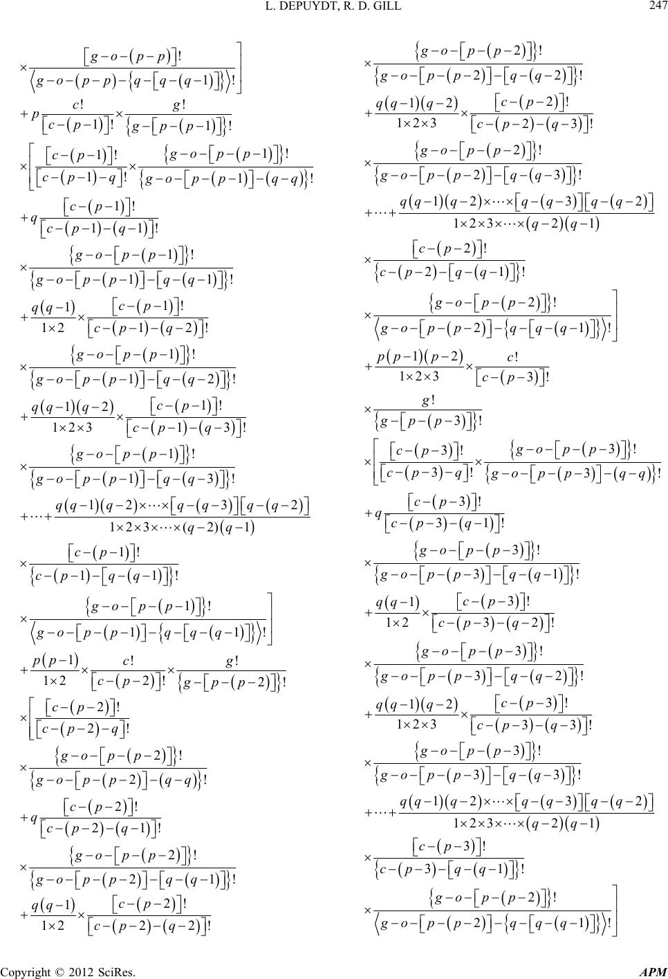




 






L. DEPUYDT, R. D. GILL 247




 


 

!
1!goppqqq

 



 


go pp
 

!!
1!
cg
p 

1!
pcpgp 









1!
1!
1! 1!
gop p
cp
cp q
g
opp qq
 

  



  






1!
11!
cp
q








qcp 

1!
11!
gop p
goppq q
  

  

 

1!
12!
cp
q








1
12
qq
cp




1!
12!q q
 

 

gop p
go p p
 
 

 



1!
13!
cp
q








12
123
qq q
cp


 

1!
13!q q
 

 


gop p
gop p

 





12
123( 2)
qqqq q
qq
 3 2
1
q q

 

 
 







1!
11!qq
 





cp
cp




1!
11!
gop p
goppq q q

  




  




 

1
12 2!
pp
cp gp

 



!!
2!
cg
p 



2!
2!
cp
cp q












2!
2!
gop p
g
opp qq
 

 



2!
21!
cp
q









qcp 

2!
21!q q


 

gop p
go p p

 

 

2!
22!
cp
q


 

1
12
qq
cp



2!
22!
gop p
goppq q
 


 

 

 



2!
12
123 23!
cp
qq q
cp q

 

 








 

2!
23!
gop p
goppq q
  

 











123 2
1232 1
qqqq qq q
qq
  

 






 

2!
21!
cp
cp qq
 








 

2!
21!
gop p
goppq q q

  




  







12 !
123 3!
pp pc
cp


 






!
3!
g
gpp











3!
3!
3! 3!
gopp
cp
cpq
g
opp qq
 

  



 









3!
31!
cp
qcp q











 

3!
31!
gop p
goppq q
  

 

 

 



 
3!
1
12 32!
cp
qq
cpq











 

3!
32!
gopp
goppq q
  

 

 

 
 
 
3!
12
123 33!
cp
qq q
cpq

 

 








 

3!
33!
go p p
goppqq
  

 











1232
1232 1
qqqq qq q
qq
  

 





 

3!
31!
cp
cp qq
 









 

2!
21!
gopp
goppqqq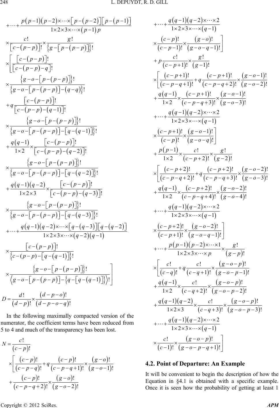

  




  



L. DEPUYDT, R. D. GILL
248





 



12
123 1
pppp p
pp
2 1p p

 


 



 

!!
!
cg
pp




!cp pgp

 

!
!
cpp
cppq


 









!
!
ppgop
g
opp
 
 p qq


 



!
1!
cpp
p q


 





qcp 
 
!
!
goppp
gopppq q
 

 

1
 
 
!
1
12 2!
cpp
qq
cpp










q

!
2!
p
q q


 

gop p
gop pp
 
 

 



!
3!
cpp
p q


 





12
123
qq q
cp


  

!
3!
p
q q


 

 
gop p
gop pp

 

 

12
123 2
qqqq q
qq
 3 2
1
q q

 

 




 



!
1!
p
qq







()
cp
cp p




!
1!q

goppp
gopppqq
  




 

 





!
!!
dpo
dpoq


In the following maximally compacted version of the
numerator, the coefficient terms have been reduced from
5 to 4 and much of the transparency has been lost.

!d
Ddp 
!
!
c
Ncp 






!!!
!1!1!
cpcp go
q
cpq cpqgo

 
 





!!cp go
2! 2!cpq go


12 2
123 1
qq q
q


 









!!
1! 1!
cp go
cp goq


 
 

!!
1! 1!
cg
pcp g 










1!1! 1!
1!2!2!
cpcp go
q
cpq cpgo
 
 
 

q







11!1!
1 23!3!
qqc po
cpq o
 
 
 
g
g





12 2
123 1
qq q
q


 









1! 1!
!!
cp go
cp goq

 
 





1!!
1 22!2!
pp cg
cp g











2!2! 2!
2!3! 3!
cpcp go
q
cpqcpq go
 

 









12!2!
1 24!4!
qqc po
cpq go
 


g






12 2
123 1
qq q
q


 









2! 2!
1! 1!
cp go
cp goq

 
 
 




12 1 !
123 !
pp pg
pgp

 







!
!!
!1!1!
p
cc
q
cq cqgop

 
go

 





1!
!
1 22!2!
qqg p
c
cq gop

 

o







12 !
!
123 3! 3!
qqqg op
c
cq gop
 

 






12 2
123 1
qq q
q


 







!
!
1! 1!
gop
c
cgopq


 


4.2. Point of Departure: An Example
It will be convenient to begin the description of how the
Equation in §4.1 is obtained with a specific example.
Once it is seen how the probability of getting at least 1

L. DEPUYDT, R. D. GILL 249
car by switching doors after doors hiding goats have been
opened is obtained in 1 case, the result can be general-
ized to all cases. In the example that will be used here,
ors Hiding Cars or Goats
It bability that a number of dif-
fewith its own de-
grand, all possible
sc of doors that hide
ei picks of doors (p =
rs (q
(o =
2).
r); 4) cccgg; 5) ccgcc; 6) ccgcg; 7) ccggc; 8)
cgcgg; 13)
cggcc; 18)
nu
the example at hand, the chance of picking a car is c/d,
, that
is, 7/
her words, the probability of a later
pick of either a goat or a car is dependent on what hap-
probearlier events
the numbers of the variables are as follows:
cars (c) = 5;
goats (g) = 7;
doors (d = c + g) = 12;
doors picked initially (p) = 3;
doors subsequently opened (o) = 2;
doors picked by switching (q) = 2.
4.3. All Possible Scenarios as Sequences of 5
Picks of Do
lies in the nature of pro
rent scenarios can be expected, each
ee of probability. In the example at h
enarios consist of 5 successive picks
ther cars or goats. There are 3 initial
3) and 2 additional picks of doors by switching doo
= 2) after 2 doors revealing goats have been opened
4.4. The 32 Possible Sequences of Picks
To be determined first are all the possible sequences of 5
picks in which either cars (c) or goats (g) are picked.
There are 32 possible sequences, as follows: 1) ccccc
(picking a car at every pick); 2) ccccg (picking 4 cars and
then 1 goat); 3) cccgc (picking 3 cars, then 1 goat, and
finally 1 ca
ccggg; 9) cgccc; 10) cgccg; 11) cgcgc; 12)
gcccc; 14) gcccg; 15) gccgc; 16) gccgg; 17)
cggcg; 19) cgggc; 20) cgggg; 21) gcgcc; 22) gcgcg; 23)
gcggc; 24) gcggg; 25) ggccc; 26) ggccg; 27) ggcgc; 28)
ggcgg; 29) gggcc; 30) gggcg; 31) ggggc; and 32) ggggg.
More generally speaking, the number 32 is obtained as
follows according to the theory of permutations. At 1st
pick, there are only 2 possible scenarios: one picks either
a car or a goat. In the 1st and 2nd picks combined, there
are 4 possible scenarios: after picking a car in the 1st
pick, one can pick either a car or a goat in the 2nd pick;
likewise, after picking a goat in the 1st pick, one can pick
either a car or goat in the 2nd pick. In other words, the
mber of possible scenarios has doubled from the 1st
pick to the 2nd pick from 2 or 21 to 4 or 22. It is easily
seen that the number of possible scenarios will likewise
double at every successive pick. Accordingly, the num-
ber of possible scenarios after 5 picks will be 25 or 32.
4.5. All Possible Scenarios as Sequences of 5
Picks of Doors Hiding Cars or Goats
The probability of each single pick is a fraction whose
numerator is either the number of available cars or the
number of available goats and whose denominator is the
number of available doors. At 1st pick, all the cars, goats,
and doors are still available for picking. Accordingly, in
that is, 5/12, and the chance of picking a goat is g/d
12.
After each pick, the denominator or the number of
doors decreases by 1, from d to d − 1, and so on. The
number of available doors decreases additionally when
doors are opened to reveal goats. In the example at hand,
the number of available doors first decreases from 12 to
9 as 3 doors are picked. The number then further de-
creases to 7 when 2 doors are opened to reveal goats.
Finally, the number decreases to 5 as 2 more doors are
picked by switching doors.
The number of available cars does not decrease when a
goat is picked. Nor does the number of available goats
when a car is picked. By contrast, the number of doors
decreases at every pick. It follows that the probability of
picking a car or a goat changes at every successive pick
because at least the number of available doors, which
constitutes the denominator of the probability of each
pick, changes.
4.6. Conditional Probability as a Property of All
Picks Preceded by Other Picks
Each pick decreases the number of the available doors as
well as either the number of available cars or the number
of available goats. In that regard, each pick of either a car
or a goat changes the probability of later picks of either a
car or a goat. In ot
pens in an earlier pick or earlier picks. An event whose
ability is affected by what happens in
is called a dependent event. Events on which other events
are dependent may be called lead events. In the Monty
Hall problem and its extensions, only the very 1st car
picks and the 1st goat picks of sequences of picks are not
dependent. An event is usually called dependent in the
context of the combined probability of 2 or more events
in which some events are dependent and others are not.
Thus, the combined probability of picking two cars in a
row is




11cd cd

. The 1st pick is the lead pick.
The 2nd pick is the dependent pick.
Earlier picks serve as conditions of the probability of
later picks. Accordingly, the general phenomenon in
which the probability of a later event is changed by an
earlier event from what its probability would have been
without that earlier event taking place is called condi-
tional probability.
For exampe, throbaility of picking a car when all
cars and all doors are still available is c/d. But once 1 car
is picked, the number of cars and doo
le pb
rs both decrease by

L. DEPUYDT, R. D. GILL
250
1, the assumption being that one cannot pick the same
door twice. The probability of picking a car therefore
changes to
 
11cd. When a goat is picked in-
stead of a car, the probability of picking a car changes
instead to

1cd. At the same time, the probability of
picking a goat chang

es to 11gd

.
The degree to which a prior event changes the prob-
ability of an event from what it would have been without
that prior event can be quantified. In the example at hand,
the change in probability from c/d to

11cd that
results from the pick of a car corresponds to a diminution
in probabilitybout 5.3%, from 5/12 to 4/11.
By contrast, the change from c/d to

of 7/132, or a
1cd that re-
sults from of a goat corresponds to an increase
in probability of 5/132, or om 5
the pick
about 3.8%, fr/12 to 5/11.
In sum, conditional probability is best measured or quan-
tified as the degree of change between a 1st event and a
2nd event whose probability depends on the 1st event.
4.7. The General Denominator of the Equation in
§4.1
It has been noted in §4.4 that there are 32 possible se-
quences of 5 picks in the example at hand. Each se-
quence of 5 picks comes with its own probability. The
specific denominator of all 32 probabilities is the same,
namely

123 4ddddod o, or in the
example at hand,
 


1212112 212 2312 2 4, or 12 × 11 ×
10 × 7 × 6. In other words, 12 × 11 × 10 × 7 × 6 is the
mon dcomenominator of all 32 probabilities. The sign ×
r of 12 factorial, or also of 12 × 11
× 3 × 2 × 1, and that 7 × 6 is the 1st
portion of 7!, or of 7 factorial, or also of 7
ppears that
12
separates the picks of doors before doors are opened
from the picks of doors after doors are opened.
What is the general form of the denominator? It ap-
pears that the expression 12 × 11 × 10 is the 1st portion
of 12!, o× 10 × 9 ×
8 × 7 × 6 × 5 × 4
× 6 × 5 × 4 × 3
× 2 × 1. In fact, the two components of the denominator
will always be portions of factorials. The need therefore
arises to represent the two components of the denomina-
tor in general forms as portions of factorials.
In that regard, 12 × 11 × 10 is nothing but 12! divided
by 9!, or 12 × 11 × 10 × 9 × 8 × 7 × 6 × 5 × 4 × 3 × 2 × 1
divided by 9 × 8 × 7 × 6 × 5 × 4 × 3 × 2 × 1. The
elimination of the common factor 9 × 8 × 7 × 6 × 5 × 4 ×
3 × 2 × 1 yields the desired 12 × 11 × 10. Likewise, 7 × 6
is the same as 7! divided by 5!, or 7 × 6 × 5 × 4 × 3 × 2 ×
1 divided by 5 × 4 × 3 × 2 × 1. The elimination of the
common factor 5 × 4 × 3 × 2 × 1 yields the desired 7 × 6.
In converting 12!/9! into a general form, it a
is the number of doors (d) and 9 is the number of the
doors (d) minus the number of doors picked before doors
are opened (p), that is, d − p. Consequently, the general
equivalent of specific 12!/9! is d!/(d − p)!. In converting
7!/5! into a general form, it appears that 7 is the number
of doors (d) minus the number of doors picked before
doors are opened (p) minus the number of opened doors
(o), that is, dpo

, and that 5 is the number of doors
(d) minus the number of doors picked before doors are
opened (p) minus the number of opened doors (o) minus
the number of doors picked after doors are opened, that is,
dpoq

. Consequently, the general equivalent of
specific 7!/5! is


d pod poq

!.
It may be concluded that the general form of the de-
nominator of the fraction that expresses the probability
that one will get at least 1 car by switching doors for any
number of d, , or q is as follows:

c, g, p, o



!
!
!!
dpo
d
dp dpoq



.
4.8. The Specific Numerators of the Probabilities
nd. Each se-
quence of 5 picks comes with its own probability. Each
of these 5 probabilities is expressed by its own fraction
and each fraction has its own numerator. The numerators
befo
doord.
of the 32 Sequences of Picks in the Example
at Hand
It has been noted in §4.4 that there are 32 possible se-
quences of 5 picks in the example at ha
of the 5 individual probabilities of all the 32 scenarios
are as follows, with × again separating the picks of doors
re doors are opened from the picks of doors after
s are opene
1) ccc × cc:



 
12 34cc ccc

 
2) ccc × cg:








12 3ccccgo

 
3) ccc × gc:




12 3cccgoc

 
4) ccc × gg:



 
12 1cccg o g o

 
5) ccg × cc:



 
123ccgcc

 
6) ccg × cg:



 
121ccgcg o

 



 
112ccgg oc 7) ccg × gc:  





11ccgg og o

2
8) ccg × gg:  




 
123cg ccc
9) cgc × cc:  




 
12 1cg ccgo 10) cgc × cg:  




 
112cg cgoc 11) cgc × gc:  


 
112cgcg og o 12) cgc × gg:  




 
123gc ccc 13) gcc × cc:  







14) gcc × cg: 12 1gc ccgo 




 
112gc cgoc 15) gcc × gc:


16) gcc × gg:


 
112gccg og o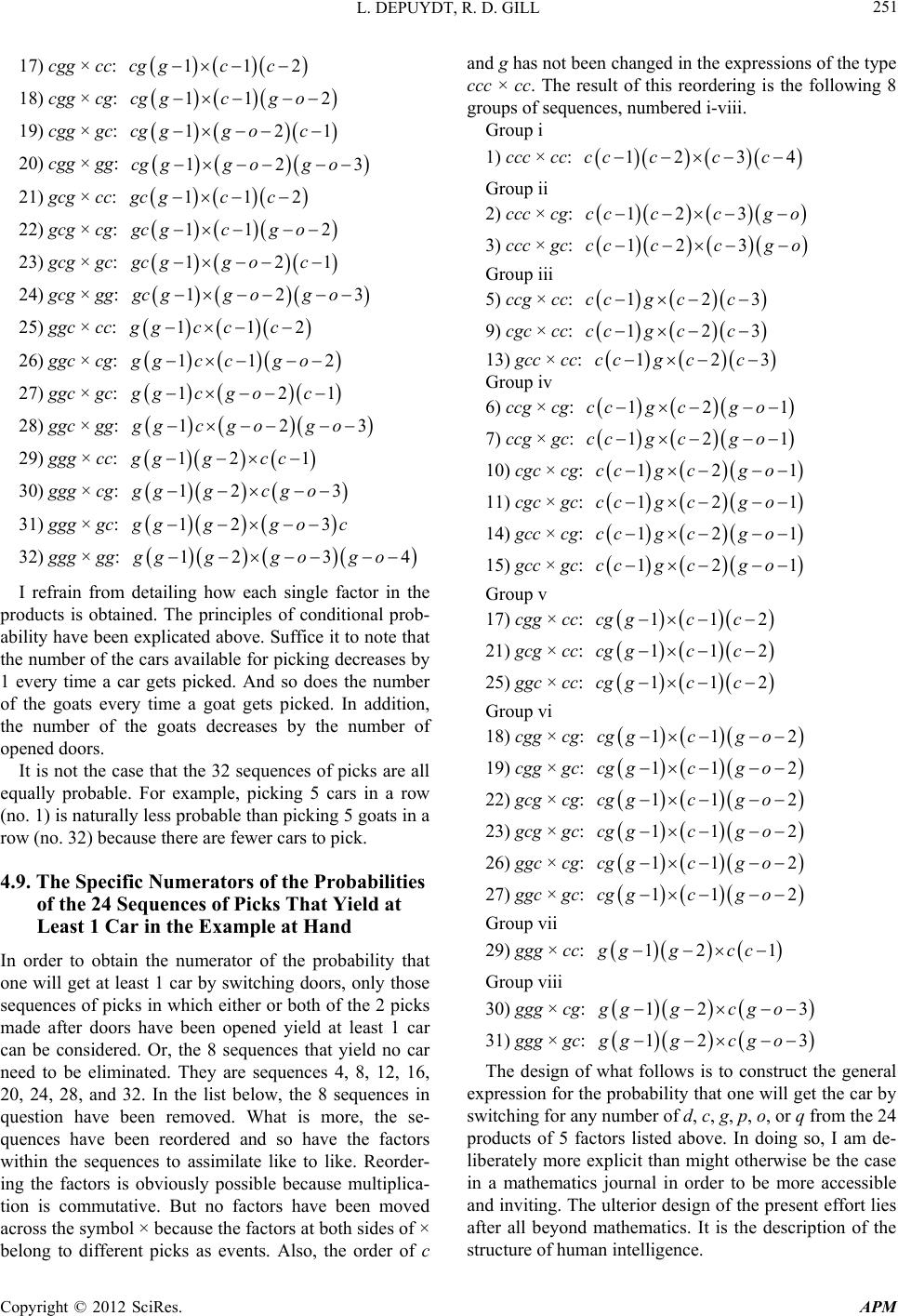


L. DEPUYDT, R. D. GILL 251
17) cgg × cc:

cgg
 
112c c
 
11 2g o 

121o c 

123g o

112c c
 
11 2g o

121o c 
 
123g o
18) cgg × cg:

cg gc
19) cgg × gc:

cg gg
20) cgg × gg: 

cg ggo 
21) gcg × cc:

gcg
22) gcg × cg:

gc gc
23) gcg × gc:

gc gg
24) gcg × gg: 

gc ggo
25) ggc × cc:






112c c  gg c
26) ggc × cg:






11 2g o 

21o c 
ggcc
27) ggc × gc:

1ggcg
28) ggc × gg:






123g o

12 1cc

3cg o
 
3
gg cg o 
29) ggg × cc:

gg g
30) ggg × cg:

12ggg
31) ggg × gc:

12
g
gggoc
 
4g o
how each single fn the
prned. The principles of condi prob-
ab explicated above. Suffice it to note that
the cars available for picking decreases by
1 r gets picked. And so dos the number
ofe a goat gets picked. Indition,
thhe goats decreases by the number of
op
at the 32 sequences of picks are all
eq. For example, picking 5 cars in a ro
(n
car by switching doors, only those
se
2, 16,
quenrs
witheorder-
32) ggg × gg: 3
 
12gggg o
I refrain from detailing actor i
oducts is obtaitional
ility have been
e number of th
every time a cae
the goats every tim ad
e number of t
ened doors.
It is not the case th
ually probablew
o. 1) is naturally less probable than picking 5 goats in a
row (no. 32) because there are fewer cars to pick.
4.9. The Specific Numerators of the Probabilities
of the 24 Sequences of Picks That Yield at
Least 1 Car in the Example at Hand
In order to obtain the numerator of the probability that
one will get at least 1
quences of picks in which either or both of the 2 picks
made after doors have been opened yield at least 1 car
can be considered. Or, the 8 sequences that yield no car
need to be eliminated. They are sequences 4, 8, 1
20, 24, 28, and 32. In the list below, the 8 sequences in
question have been removed. What is more, the se-
ces have been reordered and so have the facto
in the sequences to assimilate like to like. R
ing the factors is obviously possible because multiplica-
tion is commutative. But no factors have been moved
across the symbol × because the factors at both sides of ×
belong to different picks as events. Also, the order of c
and g has not been changed in the expressions of the type
ccc × cc. The result of this reordering is the following 8
groups of sequences, numbered i-viii.
Group i
1) ccc × cc:



 
12 34cc ccc

 
Group ii
2) ccc × cg:



 
12 3ccccgo

 
3) ccc × gc:



 
12 3ccccgo

 
Group iii
5) ccg × cc:



 
123ccgcc

 
9) cgc × cc:



 
123ccgcc

 
13) gcc × cc:

 
123ccgcc


 
Group iv






6) ccg × cg: 121ccgcg o

 
:



 
121ccgcg o 7) ccg × gc  


 
121ccgcg o 10) cgc × cg:  


 
121ccgcg o 11) cgc × gc:  


 
121ccgcg o 14) gcc × cg:  


 
121ccgcg o 15) gcc × gc:  

Group v
cc:

 
112cg gcc 17) cgg ×

 

 
112cg gcc  21) gcg × cc:


 
112cg gcc  25) ggc × cc:

Group vi

 
11 2cg gcgo 18) cgg × cg: 


 
11 2cg gcgo 19) cgg × gc:  


 
11 2cg gcgo 22) gcg × cg:

 
gc:

 
11 2cg gcgo 23) gcg ×


 
11 2cg gcgo 26) ggc × cg:  


 
11 2cg gcgo 27) ggc × gc:

 
c:

Group vii



 
12 1gg gcc  29) ggg × c

Group viii




12 3gggcg o

30) ggg × cg:  





12 3gggcg o

31) ggg × gc:

 
what follows is to constructhe general
exe probability that one will gee car by
swmber of d, c, g, p, o, or qrom the 24
prtors listed above. In doing , I am de-
lib explicit than might otherwise be the case
ins journal in order to be more accessible
anulterior design of the present effort lies
afd mathematics. It is the description of the
structure of human intelligence.
The design of t
pression for tht th
itching for any nu f
oducts of 5 facso
erately more
a mathematic
d inviting. The
ter all beyon

L. DEPUYDT, R. D. GILL
252
In turning the raexample at hand into a genel expres-
sions need to be performed: 1) the addi-
tioences of coefficients, one relating to p
an
on, two operati
n of two sequ
d the other to q, and 2) the addition of factorials. Once
these two operations have been performed, it can be de-
termined whether any simplifications are possible. The
addition of factorials has already been discussed above.
For example, a product such as

12cc c, that is, 5
× 4 × 3 in the example at hand, can first be converted
into

!3!cc, that is, 5!/(5 − 3)! or 5 × 4 × 3 × 2 × 1/2
× 1 in the example at hand. It can then be generalized to

!!ccp. It will therefore be useful to turn first to the
co
which like ha
sting of 1
On clos
2nd group consisting of nos. 2 and
permu
of the 2 doors picked,
8 groups of sequences listed in
§4
efficients, which involve “the most famous of all
number patterns” [7].
4.10. The Coefficients of the Probabilities of the
24 Sequences of Picks That Yield at Least 1
Car in the Example at Hand
In the list of products in §4.9, ins been as-
similated to like, there are 8 groups of sequences of picks
consi, 2, 3, 6, 3, 6, 1, and 2 sequences respec-
tively. How can these numbers be accounted for?
er inspection, it appears that they have every-
thing to do with how many permutations of c and g there
are in the 2 components before and after ×.
For example, in the
3, the initial product is either ccc × cg or ccc × gc. Before
×, there is 1 permutation, namely ccc. After ×, there are 2
tations, namely cg and gc. Accordingly, there are 1
× 2 or 2 members in the group.
In the 3rd group, there are 3 permutations before ×,
namely ccg, cgc, and gcc, and 2 permutations after ×,
namely cg and gc. Accordingly, there are 3 × 2 or 6
members in the group.
Furthermore, the reason that there are 3 permutations
before the symbol × in the 3rd group is that there are 3
picks of doors (p) before doors are opened and each of
the 3 picked doors, either the 1st, the 2nd, or the 3rd, can
hide the 1 goat (g) that is picked in each of the 3 se-
quences in question. Also, the reason that there are 2
permutations after the symbol × is that there are 2 picks
after doors are opened and each
either the 1st or the 2nd, can hide the 1 pick of a goat (g)
that is part of the sequences in question. The product 3 ×
2 is therefore nothing but p × q.
The members of the
.7 all share the same sequence of picks once the factors
have been reordered. In other words, there are only 8
different sequences among the 24 sequences listed in
§4.7. They are as follows.
Sequence i

12 34cc ccc
Sequence ii



 
12 3ccccgo

 
Sequence iii



 
123ccgcc

 
Sequence iv



 
121ccgcg o

 
Sequence v



 
112cg gcc 

Sequence vi



 
11 2cg gcgo 

Sequence vii




12 1gg gcc

 

Sequence viii




12 3gggcg o


 
f times that each of the 8 sequences is
represented, namely 1, 2, 3, 6, 3, 61, and 2 times re-
spectively, my be called the coefficient of the 8 se-
qun noted above that the numbers of
times in question are determined by botp and q. It ap-
pears, therefore, that each sequence is characterized by
tw one derived from p and the other de-
rived from q. It is the product of the two coefficients that
constitutes the compound coefficient of each sequence.
nd coefficients in question can now be
determined in terms of p and q by counting permutations
of c and g before and after the symbol × in each of the 8
gr
The number o
,
a
ences. It has bee
h
o coefficients,
The 8 compou
oups of sequences. The factors

112pp and


1112ppp q





 found in coefficients v-viii is
discussed in §4.14 when the example at hand is general-
ized to yield an expression that applies to all possible
cases.
Coefficient i
1 × 1 = 1 (also 1 × 1 in general)
Coefficient ii
1 × 2 = 2 or 1 × q
Coefficient iii
3 × 1 = 3 or p × 1
Coefficient iv
3 × 2 = 6 or p × q
Coefficient v
3 × 1 = 3 or

11 pp
12 

L. DEPUYDT, R. D. GILL 253
Coefficient vi
3 × 2 = 6 or

1pp
12 q 
Coefficient

vii
1 × 1 = 1 or 11
111


12
pp
p
Coefficient viii
1 × 2

= 2 or 11
2
pp qq
p



pertaining to p exhibit the sequence
1, , ,1pp . This 1st sequence returns to 1. The coefficients
pertaining equence 1, q. This 2nd se-
quence is characterized by 2 properties. First, the 2nd
se, and expands, each single
coefficient of the 1st sece. The combined sequence
 
1,,11q. Second,
to 1. The reason for the
2n that the 8 sequences of picks that
result ioutcome of not picking a car when
switchingeen removed (see §4.9
By uniting the coefficients i-viii with sequences i-viii,
on
pr
1
1
The coefficients
to q exhibit the s
nated to
quen

1,p
t re
quence is subordi
is therefo,qp
the 2nd sequence does noturn
re

11,, ,q q
d characteristic is
n the undesired
doors have b).
e obtains 8 products whose sum is the numerator of the
obability that one will get at least 1 car by switching
doors in the example at hand. The factor 1 × is explicitly
expressed for transparency.
Numerator part i: Sequence i with coefficient i
 

 
111 234cc ccc 
Numerator part ii: Sequence ii with coefficient ii
 

 
1123qccccg o 
Numerator part iii: Sequence iii with coefficient iii
 
11 23pccgcc 
Numerator part iv: Sequence iv with coefficient iv






12 1pqccg cgo 
Numerator part v: Sequence v with coefficient v
 
111

1
pp cggcc  
Numerator part vi: Sequence vi with coefficient vi
2
12 
  
11 2
12 qcggc go 
1pp
Numerator part vii: Sequence vii with coefficient vii
  
11

 
11 123 pp qgggcgo 
12 p



It appears that, of the 8 numerator parts listed above, i
an vi,
and
members of each of the 4 pairs of numerator pre
extracted and what remains is added up, one obs 4
co
tor 1
d ii share common factors, as do iii and iv, v and
vii and viii. When the common factors of the 2
arts a
tain
mpound numerator parts. In the following list, the fac-
× is again retained for transparency. Furthermore,


11
12 p
Numerator part viii: Sequence viii with coefficient viii
2 1
pp gg gcc 

1112pp p

 is the same as 1.
Compound numerator part i + ii




112cc c
  
13 4 3cc qcgo  




Compound numerator part iii + iv



1
1232 1
pccg
cc qcgo

   




Compound numerator part v + vi


 
11
12
2 1
pp cg g
c qcg


 
 
11 2c o



ii

Compound numerator part vii + vi

 
11 12
12
pp gg g
p



  
11 3ccq cgo




The sum of these 4 partial compound numerato con-
stitutes the numerator of the probability that one will get
at least 1 car byhe 4 compound nu-
m more compactly as
follows, among others because

rs
switching doors. T
erators in question can be presented
1112pp p  is
the same as 1.
i + ii:





12cc c
 
34 3cc qcgo 




iii + iv:


 
1
23 21
pc cg
cc qcgo

 




v + vi:



1
12 12
pcg g
cc qcgo

 




vii + viii:




 
12
13
g g
ccqcg o


g




Before deriving a general expression applying to all

L. DEPUYDT, R. D. GILL
254
ca he specific example at hand, it will be useful
to complete the example by computing the probability
that it involves of getting at least 1 car by switching
doors.
4.11. The Probability That One Will Get at Least
1 Car by Switching in the Example at Hand
Replacing the letters in the 4 partial compound numera-
toat the end of §4.10 by the pertinent num-
bers and resolving the subtractions and the divisions
yields the following partial numerators.
ses from t
rs obtained
i + ii:

54321225
iii + iv:

354732 234
v + vi:


357643 243
vii + viii:


76554252
The sum of these 4 sequences is, as it happens, exactly
45,000. This is the numerator of the probability that one
et at least 1 car by switching doors in the example will g
is, the prob-
ability of getting at least 1 car in the 3 initial picks (p)?
The probability of getting at least 1 car is the same as the
probability of not picking a goat 3 tims in a row in the 3
initial picks. The numerator of the probability of picking
a
at hand. The denominator is 12 × 11 × 10 × 7 × 6 (see
§4.7) or 55,440. Consequently, the probability itself is
45,000/55,440 or about 81.2%.
How does this probability compare with the probabil-
ityhe car before switching, that of getting t
e
goat 3 times in a row is




12gg
and the de-
g
nominator is




12ddd
.
The probability in question is therefore 7 × 6 × 5/12 ×
11 × 10, or 7/24, or also about 29.2%. The probability of
not picking a goat 3 times in a row, or also of picking at
least 1 car, is therefore about 70.8%.
In other words, one does somewhat increase one’s
chances of picking at least 1 car when switching doors,
from about 70.8% to about 81.2%, by a little over 10%.
4.12. A Key Difference between Monty Hall 1.0
and 2.0 and Monty Hall 3.0 and Higher
What makes Monty Hall 3.0 much more interesting than
Monty Hall 1.0 and 2.0 is t Monty Hall
1.0 and 2.0, o
he following. In
ne always increases one’s chances of get-
tin
g may ei-
th
some titillating variants of the expanded Monty Hall
4.13.
g 1 car by switching doors when doors are opened to
reveal goats [8]. But in Monty Hall 3.0 and higher, de-
pending on the conditions and what the desired aim is,
one’s chances of being successful by switchin
er decrease or increase. A full study of these conditions
exceeds the scope of the present paper. A complete un-
derstanding of them should make the construction of
problem possible. Some reflections follow in §6.
First Generalization of the Numerator in
the Example at Hand by Introducing
Factorials
So far, what has been obtained in regard to the example
at hand is 4 compound products, the following (§4.10).
i + ii:




 
12
34 3
ccc
cc qcgo

 




iii + iv:


 
1
23 21
pc cg
cc qcgo

 




v + vi:


1pcgg 

 
12 12cc qcgo




ii: vii + vi




 
12
13
gg g
ccqcg o






of these four compound products constitutes
thtor of the probability that one will get at least
1 car by switching doors in the example at hand of the
extended Monty Hall problem. How to pr from
here?
ctive thinking, there is no need for many ex-
amples or many experiments to obtain the truth about a
matter as there is in inductive thinking. The truth can be
seen in, and generalized from, a single example. In de-
riving the general truth about the probability at hand
frmple at hand, the following observation can
serve as a point of departure.
The number of cars or goats decreases by 1 with each
successive pick of 1 car or 1 goat. Accordingly, the se-
qu
The sum
e numera
oceed
In dedu
om the exa
ences of products of factors listed above can be inter-
preted as incomplete or partial factorials or snippets of
factorials. For example, the sequence of factors in the
product




12ccc

, in this case 5 × 4 × 3, is part of
the factorial c!, in this case 5 × 4 × 3 × 2 × 1, or 5!. In
cases in which there are fewer cars or goats than there are
picks, a factor will reduce to zero and the probability of
the sequence of picks of events in question will be 0.
In a next step, the partial factorial 5 × 4 × 3 can be ob-
tained by dividing the complete factorial 5 × 4 × 3 × 2 ×
1 by the rest of the factorial, namely 2 × 1, or 2!. In this
case,




12ccc

 equals c! divided by 2!. However,
if c were 6 and not 5,

 
12cc c would equal c!
divided by 3!. It is therefore desirable to generalize the
expression of the division of a complete factorial by a
partial factorial to any c.

L. DEPUYDT, R. D. GILL 255
In that regard, it appears that the relation between the
number of the complete factorial c! and the number of
the partialways the same. The number of
the partial factorial is always 3c because the number
of the picks is always 3, however many cars there are.
The divisions of complete factorials by partial factorials
can therefore be generalized by expressing the number
al factorial is
of
th
et
e partial factorial in its relation to the number of the
complete factorial. In the case at hand, the partial factor
can be expressed as

3!c and the division of the
compl the partial factorial as e factorial by


3!cc.
By this same procedure, umerators listed
above can be converted into the following equivalents.
i + ii:
the 4 partial n








3! 3!!
!
3! 5!4!1!
ccgo
cq
cc cgo


 

 

iii + iv:


 


!!
2! 1!
2! 2!1!
4! 3!2!
cg
pcg
ccgo
q
ccgo








v + vi:

!!
1! 2!
cg
pcg 







1! 1! 2!
3! 2!3!
ccgo
q
ccgo






vii + viii:



3!
!
4!
go
go






!!
3! 2! 1!
gc c
q
gc c



 

By being converted into !3!cc, axpression
cc been generalized to a certain
in that it only applies when
p all the terms in the equivalents listed above
on when p is 3 and q is 2. The need is for con-
verting the terms into expressions that apply to any p and
any c.
But before proceeding to the generalization to any p
and any c, it is necessary to detail the general structure of
coefficients. The coefficients relate to how many times
eances of picks are taken. They
ha been discussed provisionally in §4.10. The
need at this point is for a general treatment.
4.14. The Structure of Coefficients
ficients of t
d in Pascal’s Arithmetical Triangle. How these
nu
many co-
efficients there are) of a compound quantity consisting of
er n, that is,
how o
o
y can b
n e
such as
degree. Bu

12c has
t it is still specific
is 3. In fact,
ly apply
ch of the possible seque
ve already
The coefhe Equation pertaining to the ex-
tended Monty Hall problem exhibit the same structure as
the coefficients of the power of a compound quantity that
consists of two members, that is,

n
ab. The basic
facts about this structure have been well-known for more
than four centuries. They involve the numbers that are
also foun
mbers are obtained may be briefly reviewed below to
make the present account fully self-sufficient. A particu-
larly lucid and at the same time delightfully parsimoni-
ous presentation of the matter at hand is Euler’s in his
“Elements of Algebra” [9].
The number of the coefficients (that is, how
2 members a and b raised to the pow
n

ab, equals the number of the power of the com-
pound quantity, that is, n, augmented by 1, or n + 1. The
number n + 1 is also the number of ways in which the 2
members can be arranged in regard toften they are
taken. Thus,

5
ab yields 6 coefficients, that is, the
power 5 plus 1. Accordingly, there are 6 arrangements
when it comes to how often the 2 members a and b of the
compound quantity can be taken. One can take 5 times a
and 0 times b, 4 times a and 1 time b, 3 times a and 2
times b, 2 times a and 3 times b, 1 time a and 4 times b,
and 0 times a and 5 times b. If the items are multiplied,
the 6 arrangements are as follows: aaaaa, aaaab, aaabb,
aabbb, abbbb, and bbbbb, which can also be written as a5,
a4b, a3b2, a2b3, a1b4, and b5. The 6 arrangements are the 6
main terms of the compound quantity. Each main term
has its wn coefficient.
The coefficient numbers (that is, what the numbers of
each individual coefficient are) are determined by the
number of the ways in which the 2 members of the com-
pound quantite ordered in each of the arrange-
ments that relate to how often they are taken. The ele-
ments can be ordered in only 1 way in aaaaa. Accord-
ingly, the coefficient of a5 is 1. There are 5 ways of or-
dering the elements in aaaab, namely aaaab, aaaba, aa-
baa, abaaa, and baaaa. Accordingly, the coefficient of
a4b is 5. Along these same lines, the coefficients of a3b2,
a2b3, a1b4, and b5 can be determined to be 10, 10, 5, and 1
respectively.
In sum,

5
ab

equals a5 + 5a4b + 10a3b2 + 10a2b3 +
5a1b4 + b5.
Coefficient numbers can also be obtained as follows
without having to count ways of ordering elements. If all
the letters are different, as in abcde, the number of ways
in which the letters can be ordered is the factorial of the
number of letters, in this case 5! If 2 letters are the same,
as in abcdd, 5! needs to be divided by 2! Therefore, in
aaabb, 5! needs to be divided by both 3! and 2! The re-
sult is 10. Furthermore, 5!/(3!2!), or (5 × 4 × 3 × 2 × 1)/
(3 × 2 × 1× 2 × 1), equals (5 × 4 × 3)/(1 × 2 × 3). The 6
coefficients 1, 5, 10, 10, 5, and 1 therefore equal 1, 5/1,
(5 × 4)/(1 × 2), (5 × 4 × 3)/(1 × 2 × 3), (5 × 4 × 3 × 2)/(1
× 2 × 3 × 4), and (5 × 4 × 3 × 2 × 1)/(1 × 2 × 3 × 4 × 5)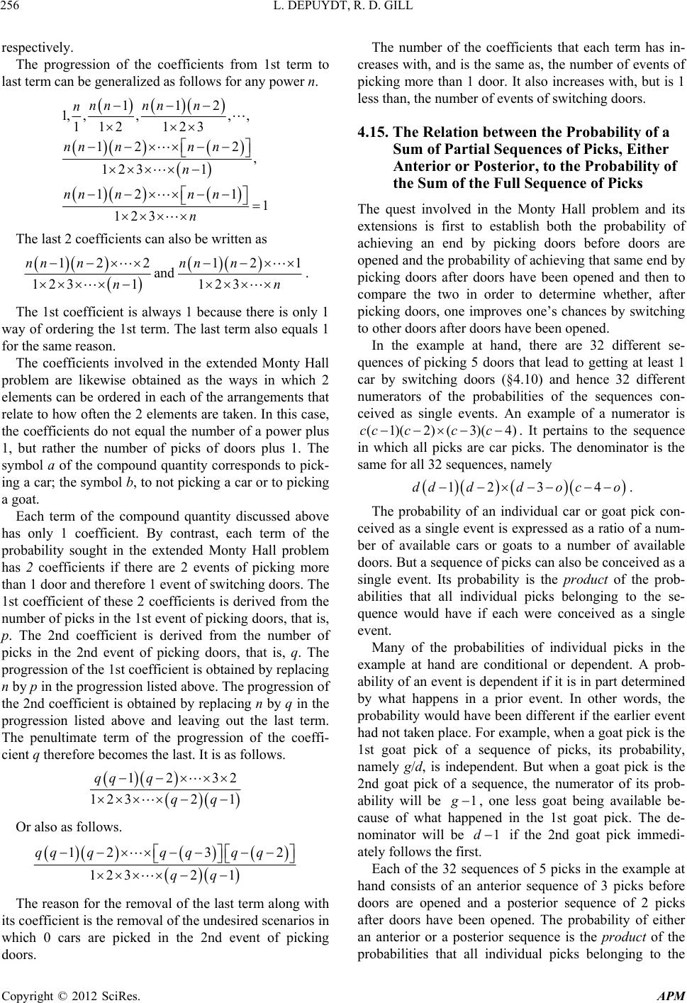

L. DEPUYDT, R. D. GILL
256
respectively.
The progression of the coefficients from 1st term to
lan be gest term caneralized as follows for any power n.
 


 
112
1, ,,,,
112123
122
,
123 1
12 1
1
12 3
nnnnn
n
nnnnn
n
nnnnn
n








 








The last 2 coefficients can also be written as
 
  
12212 1
and
123 1123
nn nnn n
nn




.
The 1st coefficient is always 1 because there is only 1
way of ordering the 1st term. The last term also equals 1
for the same reason.
The coefficients involved in the extended Monty Hall
problem are likewise obtained as the ways in which 2
elements can be ordered in each of the arrangements that
relate to how often the 2 elements are taken. In this case,
the coefficients do not equal the number of a power plus
1, but rather the number of picks of doors plus 1. The
symbol a of the compound quantity corresponds to pick-
ing a car; the symbol b, to not picking a car or to picking
a goat.
d above
has only 1 coefficient. By contrast, each term of the
probability sought in the extended Monty Hall problem
has 2 coefficients if there are 2 events of picking more
th
1st event of picking doors, that is,
p.
Each term of the compound quantity discusse
an 1 door and therefore 1 event of switching doors. The
1st coefficient of these 2 coefficients is derived from the
number of picks in the
The 2nd coefficient is derived from the number of
picks in the 2nd event of picking doors, that is, q. The
progression of the 1st coefficient is obtained by replacing
n by p in the progression listed above. The progression of
the 2nd coefficient is obtained by replacing n by q in the
progression listed above and leaving out the last term.
The penultimate term of the progression of the coeffi-
cient q therefore becomes the last. It is as follows.
 

12 32
1232 1
qq q
qq




Or also as follows.
 



1232
1232 1
qqqq qq q
qq
 





The reason for the removal of the last term along with
its coefficient is the removal of the undesired scenarios in
which 0 cars are picked in the 2nd event of picking
doors.
The number of the coefficients that each term has in-
creases with, and is the same as, the number of events of
picking more than 1 door. It also increases with, but is 1
less than, the number of events of switching doors.
4.15. The Relation between the Probability of a
Sum of Partial Sequences of Picks, Either
Anterior or Posterior, to the Probability of
Full Sequence of Picks
The quest involved in the Monty Hall problem and its
extensions is first to establish both the probability of
achieving an end by picking doors before doors are
op
on-
s
the Sum of the
ened and the probability of achieving that same end by
picking doors after doors have been opened and then to
compare the two in order to determine whether, after
picking doors, one improves one’s chances by switching
to other doors after doors have been opened.
In the example at hand, there are 32 different se-
quences of picking 5 doors that lead to getting at least 1
car by switching doors (§4.10) and hence 32 different
numerators of the probabilities of the sequences c
ceived as single events. An example of a numerator i
(1)(2) (3)(4)cc ccc

 . It pertains to the sequenc
ich all picks are car picks. The denominator is the
or all 32 sequences, namely
e
in wh
same f





 
12 34ddddo co

  .
The probability of an individual car or goat pick con-
ceived as a single event is expressed as a ratio of a num-
ber of available cars or goats to a number of available
doors. But a sequence of picks can also be conceived as a
single event. Its probability is the product of the prob-
abilities that all individual picks belonging to the se-
quence would have if each were conceived as a single
ev
probability would have bee
cks, its probability,
namely g/d, is independent. But when a goat p is the
2nd goat pick of a sequence, the numerator ofprob-
ab
ent.
Many of the probabilities of individual picks in the
example at hand are conditional or dependent. A prob-
ability of an event is dependent if it is in part determined
by what happens in a prior event. In other words, the
n different if the earlier event
had not taken place. For example, when a goat pick is the
1st goat pick of a sequence of pi
ick
its
ility will be 1
g

, one less goat being available be-
cause of what happened in the 1st goat pick. The de-
nominator will be 1d

if the 2nd goat pick immedi-
ately follows the first.
Each of the 32 sequences of 5 picks in the example at
hand consists of an anterior sequence of 3 picks before
doors are opened and a posterior sequence of 2 picks
after doors have been opened. The probability of either
an anterior or a posterior sequence is the product of the
probabilities that all individual picks belonging to the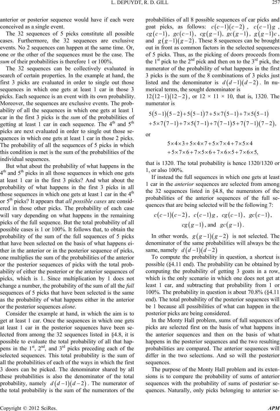

L. DEPUYDT, R. D. GILL 257
anterior or posterior sequence would have if each were
conceived as a single event.
The 32 sequences of 5 picks constitute all possible
cases. Furthermore, the 32 sequences are exclusive
events. No 2 sequences can happen at the same time. Or,
one or the other of the sequences must be the case. The
sum of their probabilities is therefore 1 or 100%.
The 32 sequs can be collectively evaluated in
search of certain properties. In the example at hand, the
first 3 picks are eved in order to single out those
sequences in which on
ence
aluat
e gets at least 1 car in those 3
pi
ences of 5 picks in which
th
ut the
pr
e multiplication by 1 does not
c
cks. Each sequence is an event with its own probability.
Moreover, the sequences are exclusive events. The prob-
ability of all the sequences in which one gets at least 1
car in the first 3 picks is the sum of the probabilities of
getting at least 1 car in each sequence. The 4th and 5th
picks are next evaluated in order to single out those se-
quences in which one gets at least 1 car in those 2 picks.
The probability of all the sequ
is condition is met is the sum of the probabilities of the
individual sequences.
But what about the probability of what happens in the
4th and 5th picks in all those sequences in which one gets
at least 1 car in the first 3 picks? And what abo
obability of what happens in the first 3 picks in all
those sequences in which one gets at least 1 car in the 4th
or 5th picks? It appears that all possible cases are consid-
ered in those other picks. The probability of each case
will vary depending on what happens in the remaining
picks of the full sequence. But the total probability of all
possible cases is 1 or 100%. It follows that, to obtain the
probability of the sum of the full sequences of 5 picks
that have been selected on the basis of what happens ei-
ther in the anterior or in the posterior sequence of picks,
one multiplies the sum of the probabilities of the anterior
or the posterior sequences of picks with the total prob-
ability of either the posterior or the anterior sequences of
picks, which is 1. Sinc
hange a number, the probability of the sum of all the full
sequences of 5 picks that have been selected is the same
as the probability of what happens either in the anterior
or the posterior sequences alone.
Consider the example at hand, in which the aim is to
get at least 1 car. Once the sequences in which one gets
at least 1 car in the posterior sequences have been se-
lected from among the 32 sequences listed in §4.8, it is
possible to evaluate the total probability of all that hap-
pens in the 1st, 2nd, and 3rd picks preceding each of the
selected sequences. This total probability is the sum of
all the probabilities of each of the ways in which the first
3 doors can be picked. The denominator shared by all
these probabilities is also the denominator of the total
probability, namely



12ddd. The numerator of
the total probability is the sum of the numerators of the
probabilities of all 8 possible sequences of car picks and
goat picks, as follows:

12cc c,


1cc g,


1cg c

,


1gc c

,


1cgg,

1gcg,


1
g
gc,
and




12gg g

. These 8 sequences can be brought
out in front as common factors in the selected sequences
of 5 picks. Thus, as the picking of doors proceeds from
the 1st pick to the 2nd pick and then on to the 3rd pick, the
numerator of the probability of what happens in the first
3 picks is the sum of the 8 combinations of 3 picks just
listed and the denominator is
 
12ddd. In nu-
merical terms, the sought denominator is




12 121122

, or 12 × 11 × 10, that is, 1320. The
numerator is








 
55 1 5255 175 7517 55 1
5771 75577172,

 
or
543547
5 76

71771
 
574754
7656 75765,

 

 
that is 1320. The total probability is hence 1320/1320 or
1, or also 100%.
If instead the full sequences in which one gets at least
1 car in the anterior sequences are selected from among
the 32 sequences listed in §4.8, the numerators of the
probabilities of the anterior sequences of the full se-
quences that are being selected will be the following 7:




12cc c,


1cc g,

1cgc,


1gcc

,



1cg g

, and

1gcg.
In other words,

 
12gg g

 is not selected. The
denominator of the same probabilities will always be the
, namely




12ddd same


compute the probability in question, a shortcut is
possible (§4.11 end). The probability can be obtained by
computing the probability of getting 3 goats in a row,
the anterior sequces and then on the
happens in the posterior ces and to resulting
probabilities are compared. e anterior sequences will
di elections. And
of the Monty Hall problem and its exten-
si
To
which is the only scenario in which one does not get at
least 1 car, and subtracting that probability from 1 or
100%. The probability in question is about 70.8% (§4.11
end). The total probability of the posterior sequences will
be 1 because all possibilities of what can happen in the
posterior picks are being considered.
In the Monty Hall problem, sums of full sequences of
picks are selected first on the basis of what happens in
en basis of what
sequenhe tw
Th
ffer in the two sso will the posterior
sequences.
The purpose
ons is to compare the probability of sums of anterior
sequences with the probability of sums of posterior se-
quences. Naturally, only picks belonging to anterior se-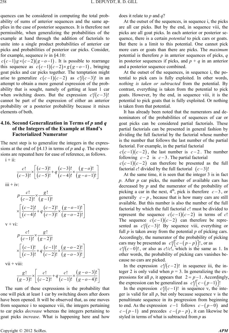

L. DEPUYDT, R. D. GILL
258
quences can be considered in computing the total prob-
ability of sums of anterior sequences and the same ap-
plies in the case of posterior sequences. It is therefore not
permissible, when generalizing the probabilities of the
example at hand through the addition of factorials to
unite into a single product probabilities of anterior car
picks and probabilities of posterior car picks. Consider,
for example, sequence iv in §4.10:
 
121ccgcg o. It is possible to rearrange
this sequence as
 
12 1cccggo, bringing
goat picks and car picks together. The temptation might
arise to generalize
 
12cc c as

!3!cc in an
attempt to obta
ab
in a more general expression of the prob-
ility that is sought, namely of getting at least 1 car
when switching doors. But the expression


!3!cc

cannot be part of the expression of either an anterior
probability or a posterior probability because it mixes
elements of both.
4.16. Second Generalization in Terms of p and q
of the Integers of the Example at Hand’s
Factorialized Numerator
The next step is to generalize the integers in the expres-
sions at the end of §4.13 in terms of p and q. The expres-
sionsr e are repeated here foase of reference, as follows.
i + ii:








3! 3!!
!
3! 4!
ccgo
c
cc






iii + iv:

5! 1!
qcgo








!!
2! 1!
2!
cg
pcg
c






2! 1!
4! 3!2!
c go
q
ccgo
 



v + vi:







!!cg
p
1! 2!
1! 1!2!
3! 2!3!
cg
cc go
q
ccgo




 



vii + viii:



3!
!
4!
go
c cgo




 

The sum of these expressions is the probability that
one will pick at least 1 car by switching doors after doors
have been opened. It will be observed that, as one moves
from sequence i to sequence viii, the integers pertaining
to car picks decrease whereas the integers pertaining to
goat picks incr eas e. What is happening here and how
does it relate to p and q?
At the outset of the sequences, in sequence i, the picks
are all car picks. But by the end, in sequence viii, the
picks are all goat picks. In each anterior or posterior se-
quence, there is a certain potential to pick cars or goats.
But there is a limit to this potential. One cannot pick
more cars or goats than there are picks. The maximum
potential is therefore p in anterior sequences of picks, q
in posterior sequences if picks, and p + q in an anterior
and a posterior sequence combined.
At the outset of the sequences, in sequence i, the po-
te
!!
3! 2! 1!
gc c
q
g
ntial to pick cars is fully exploited. In other words,
nothing is taken or subtracted from the potential. By
contrast, everything is taken from the potential to pick
goats. However, by the end, in sequence viii, it is the
potential to pick goats that is fully exploited. Or nothing
is taken from that potential.
It has already been noted that the numerators and de-
nominators of the probabilities of sequences of car or
goat picks can be considered partial factorials. These
partial factorials can be presented in general fashion by
dividing the full factorial by the factorial whose number
is the number that follows the last number of the partial
factorial. For example, in the partial factorial




12ccc

, the last number is 2c. The number
following 2c

is 3c

. The partial factorial




12ccc

 can therefore be presented as the full
factorial c! divided by the full factorial

3!c
At the same time, it is seen that the integer 3 is in fact
p. After p car picks, the number of available cars has
decreased by p and the numerator of the probability of
picking a car in the next, 4th, pick is therefore 3c

, or
generally cp

, because that is how many cars are still
available. But this number is also the number of the full
factorial by which the full factorial c! must be divided to
represent the sequence

 
12cc c in terms of c!
The sequence




12ccc

 can therefore be repre-
sented as


!3!cc

By sequence viii, everything or
full p is taken away from the potential p of picking cars.
Accordingly, the numerator of the probability of picking
cars may be presented as

!!cc pp

, or as


!0!cc, or
s, theshes be-
cause no cars a
also as c!/c!, which is the same as 1. In
other word probability of picking cars vani
re picked.
In the expression


!2!cc in seqii, tuence ihe in-
teger 2 is only valid when p = 3. In generalizing the ex-
pressions for all p, it appears that 21p. Accordingly,
the expression can be generalized as

!1!cc p 

In the expression


!1!cc

in sequence v, nte-
ger is valid for all p, but only because sequence v is the
penultimate sequence in its progression from beginning
to end. As the expression 1c follows

0cp and
the i


1cp

 and precedes t can likewise be

cpp, i
styled in terms of what is subtracted from p as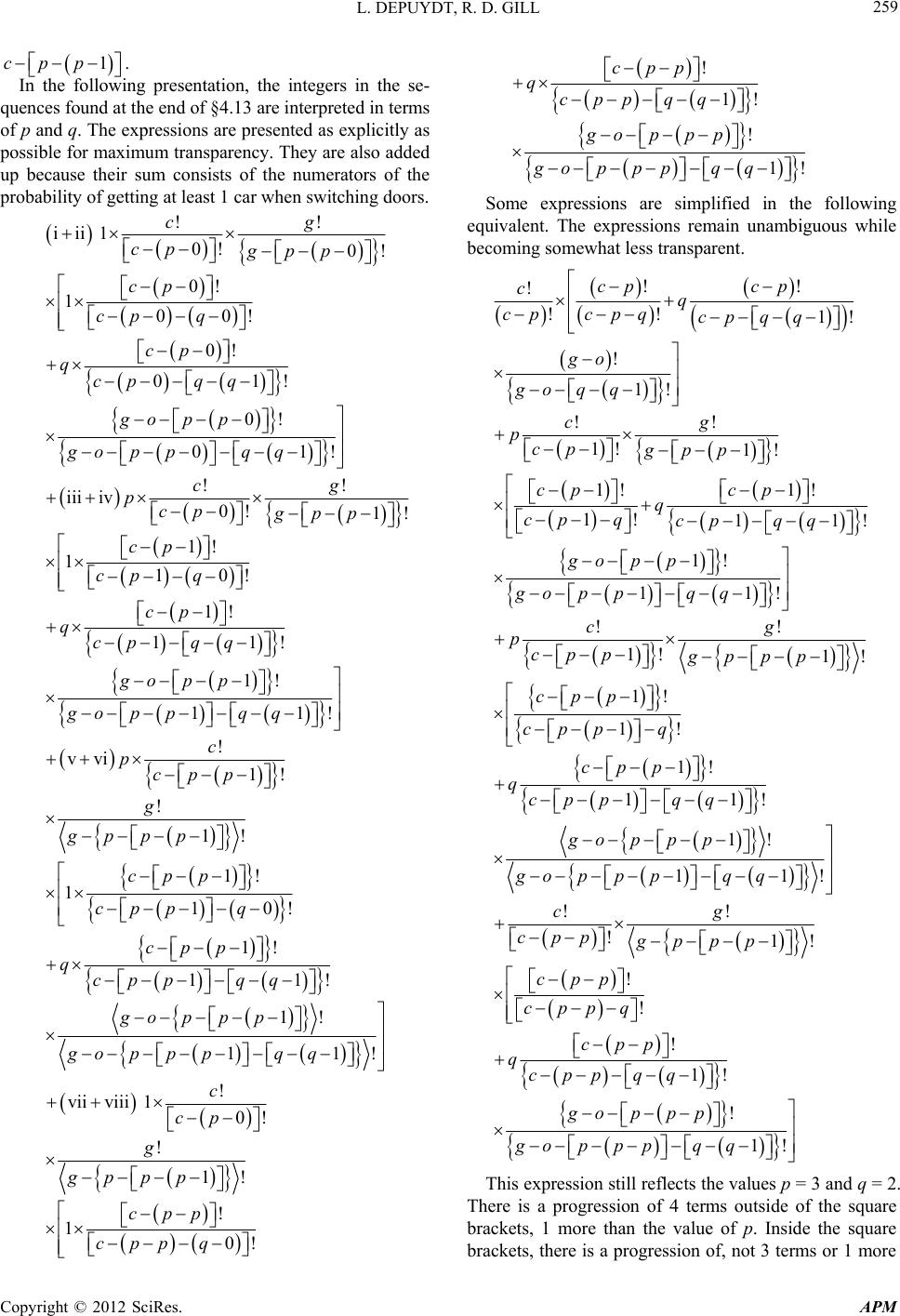

L. DEPUYDT, R. D. GILL 259

1cpp 

In the fpresentation, the integers in the se-
quences found at the end of §4.13 are interpreted in terms
of p and q. The expressions are presented as explicitly as
possible for maximum traare also
e their sum consists of the numerators of the
probability of getting at least 1 car when switching doors.
.
ollowing
nsparency. They added
up becaus


 

  

!c!g


ii i 10! 0!
cp gpp







0!
100
cp
cpq




 !



 

0!
01!
cp
qcp qq
 

 


 


0!p 
01 !
go p
gopqq

 



  

p 

  

!!
iii iv0!1!
cg
pcp gpp  


 




1!
110!
cp
cpq








 

1!cp 

11 !
qcp qq  







1!
11! q q




  




gopp
gop p
  


!
1!
c
cpp 



vv i p  
!
1! p  





g
gpp

1!
10!
p
q
 

 





1cp
cpp






1!
11!
p
qq





cp
qcpp

 

 

1!
11! q



go pp p
go pp pq
  



  

 




!
0!
c
cp





viiviii 1

!
1!p 



g
gpp

!
0!
cpp
p q




1cp





!
1!
cpp
qcpp qq
 

 








 

!
1!
gop pp
gopppq q
  

 

 

 
Some expressions are simplified in the following
equivalent. The expressions remain unambiguous while
becoming somewhat less transparent.






!!
!
!! 1!
cp cp
cq
cp cpqcpq q




 






!
1!
go
goq q





 




 

!!
1! 1!
cg
pcpgpp 
 









 

1! 1!
1! 11!
cp c
q
cp qcp qq
 
 
 


 


 


p


 

1!gop p   



11 ! go ppq q    

 

 

 

!!
1!
cg
pcppgpp 
 
 
 
1!p 






1!
1!
cpp
cppq




 







 

1!
11!
cpp
qcppqq




 
 




 

1!
11!
go pp p
gopppq q

   




 


 

!!
!1!
cg
cpp gppp



 
 



!
!
cpp
cppq














 

!
1!
cpp
qcpp qq
 









 

!
1!
gop pp
gopppq q

 



 


 

 
This expression still reflects the values p = 3 and q = 2.
There is a progression of 4 terms outside of the square
brackets, 1 more than the value of p. Inside the square
brackets, there is a progression of, not 3 terms or 1 more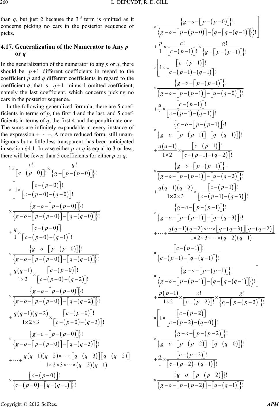

L. DEPUYDT, R. D. GILL
260
than q, but just 2 because the 3rd term is omitted as it
concerns picking no cars in the posterior sequence of
picks.
4.17. Generalization of the Numerator to Any p
or q
In the generalization of the numerator to any p or q, there
d be 1p different coefficients in regard to the
coefficient p and q different coefficients in regard to the
coefficient , that is, 1q minus 1 omitted coefficient,
namely the last coefficient, which concerns picking no
cars in the posterior sequence.
In the following generalized formula, there are 5 coef-
ficients in terms of p, the first 4 and the lasef-
ficients in terms of q, the first 4 and the penultimate one.
Th
shoul
q
t, and 5 co
e sums are infinitely expandable at every instance of
the expression + ··· +. A more reduced form, still unam-
biguous but a little less transparent, has been anticipated
in section §4.1. In case either p or q is equal to 3 or less,
there will be fewer than 5 coefficients for either p or q.
 

!!
1cg
c



0! 0! pgpp  
 

 

0!
1cp
c




00 ! pq








 


0!
00!
opp
goppq q
 

  

g


0!
101!
cp
q
cpq


 




 

0!
01!
gopp
goppq q
 

 

 

0!
1
12 02!
cp
qq
cpq



 



 

0!go p p 


02go ppq q   

!




0!
!
cp
qq q
cpq

 

 






12
12 303

0!
03!
q q


 


gopp
gop p

 

 



12
123 2
qqqq q
qq
 3 2
1
q q

 

 




 




0!
01! qq





cp
cp




 

0!
01!
gopp
goppqq q

 




  


 

!!
11!
pc g
cp gpp
 
 
 


1!



1!
111!
cp
cp q














 

1!
10!
gop p
goppq q
 

 

 
 




1!
111!
cp
q
cp q


 








 

1!
11!
gopp
goppq q
 

  

 

 




1!
1
12 12!
cp
qq
cp q












 

1!
12!
gop p
goppq q
 

 

 

 
 
 
1!
12
123 13
cp
qq q
cp q

 

 !








 

1!
13!
gopp
goppq q
 

 

 
 








1232
1232 1
qqqq qq q
qq
  

 


 


 

1!
11
cp
cp qq
 

 !






 


1!
11
gopp
goppqqq

 




  


！ 


 

1!!
12 2! 2!
pp cg
cp gpp









2!
120!
cp
cp q














 

2!
20!
gopp
goppq q
 

 

 
 




2!
121!
cp
q
cp q


 








 

2!
21!
gopp
goppq q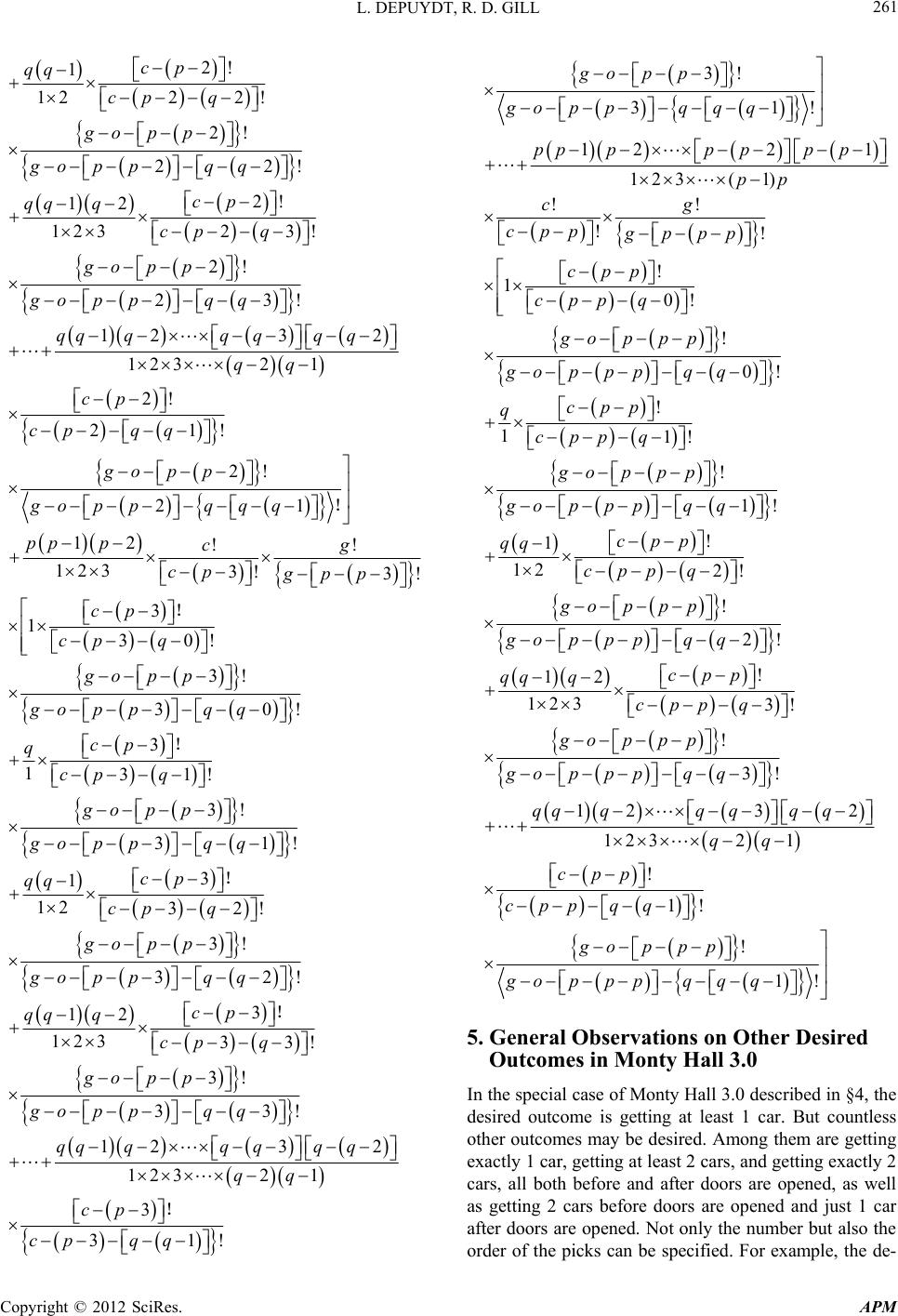
 

 

 
 


L. DEPUYDT, R. D. GILL 261




2!
1
12 22!
cp
qq
cp q










2!
22!q q
 

 

gop p
gop p

 

 

2!
23!
cp
q








12
123
qq q
cp


 

2!
23!q
  

 

 
gop p
gop pq
 

12
123 2
qqqq q
qq
 

 



3 2
1
q q






2!
21!
qq
 





cp
cp





2!
21 q



 


！
gop p
goppq q
   

 


 

12 !!
123 3! 3!
pp pcg
cp gpp


 

 




3
30!
cp
q




！




1cp






3!
30!q q
 

 

gop p
gop p

 



3
31!
cp
q




！




1
q
cp
 

3!
31!qq
 

 

gop p
gop p
 
 

 

3
32!
cp
q




！




1
12
qq
cp




3!
32!q q
 

 

gop p
gop p

 

 

3
33!
cp
q




！




12
123
qq q
cp


 

3!
33!q q
 



 

gop p
gop p


 

12
123 2
3 2qqqq qq q
qq
  

 






1

3
31! qq
 



！


 

cp
cp


3!
31!
go p
goppqq q

 

p



  








12 1
123( 1)
pppppp p
pp
 

 




2


!!
!!
cg
cpp gppp





 




!
10!
cpp
cpp q














 

!
0!
gop pp
gopppq q
 


 

 

 



!
11!
cpp
q
cpp q


 








 

!
1!
gop pp
gopppq q
  

 

 

 




!
1
12 2!
cpp
qq
cpp q












 

!
2!
gop pp
gopppq q
 


 

 

 
 
 
!
12
123 3!
cpp
qq q
cpp q

 

 








 

!
3!
gop pp
gopppq q
  

 











123 2
1232 1
qqqqqq
qq
 

 



q


 

!
1!
cpp
cpp qq
 








 

!
1!
goppp
gopppqqq








  


5. General Observations on Other Desired
Outcomes in Monty Hall 3.0
In the special case of Monty Hall 3.0escribed in §4, the
desired outcome is getting at least 1 car. But countless
other outcomes may be desired. Among them are getting
exactly 1 car, getting at least 2 cars, and getting exactly 2
cars, all both before and after doors are opened, as well
as getting 2 cars before doors are opened and just 1 car
after doors are opened. Not only the numbebut also the
order of the picks can be specified. For example, the de-
d
r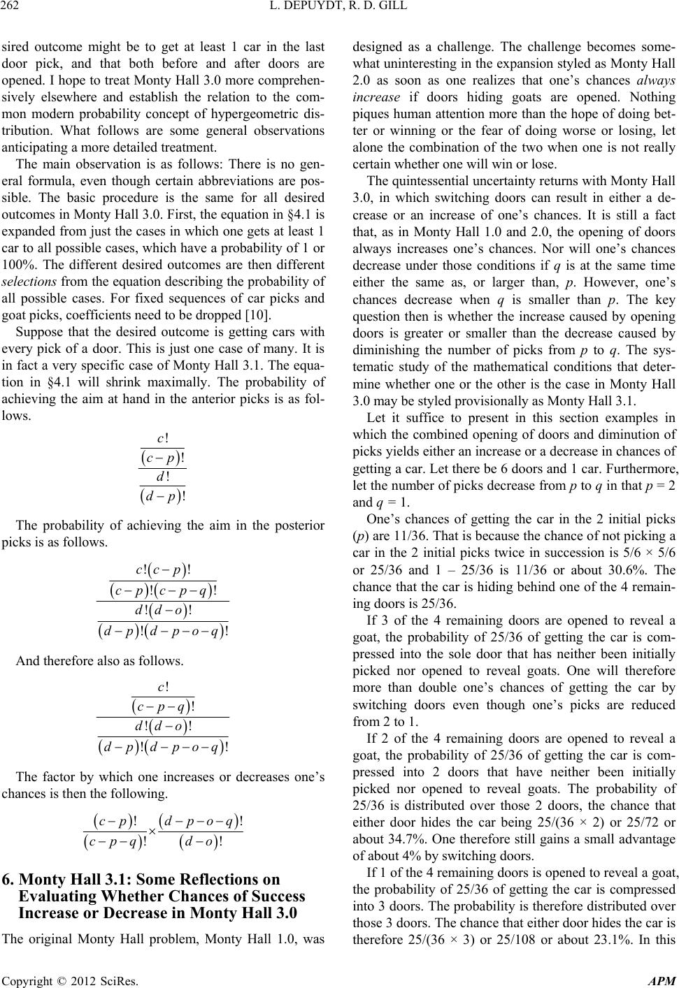

L. DEPUYDT, R. D. GILL
262
sired outcome might be to get at least 1 car in the last
door pick, and that both before and doors are
opened. I hope to treat Monty Hall 3.0 more comprehen-
sively elsewhere and establish the relation to the com-
mon modern probability concept of hypergeometric dis-
tribution. What follows are some general observations
anticipating a more detailed treatment.
The main observation is as is no gen-
eral formula, even though certain abbreviations are pos-
sible. The basic procedure is the same for all desired
outcomes in Monty Hall 3.0. First, the equation in §4.1 is
expanded from just the cases in which one gets at least 1
car to all possible cases, which have a probability of 1 or
nt
of
allof car picks and
after
follows: There
100%. The different desired outcomes are then differe
selections from the equation describing the probability
possible cases. For fixed sequences
goat picks, coefficients need to be dropped [10].
Suppose that the desired outcome is getting cars with
every pick of a door. This is just one case of many. It is
in fact a very specific case of Monty Hall 3.1. The equa-
tion in §4.1 will shrink maximally. The probability of
achieving the aim at hand in the anterior picks is as fol-
lows.


!
!
!
!
c
cp
d
dp


The probability of achieving the aim in the posterior
picks is as follows.

 


!!
!!
!!
!!
ccp
cpcpq
ddo
dpdpoq




And therefore also as follows.



!
!
!!
c
cpq
ddo


!!dpdpoq
The factor by which one increases or decreases one’s
chances is then the following.




!!
!!
dpoq
do


6. Monty Hall 3.1: Some Reflections on
Evaluating Whether Chances of Success
Increase or Decrease in Monty Hall 3.0
Th
nge. The challenge becomes some-
what uninteresting in the expansion styled as Monty Hall
2.0 as soon as one realizes that one’s chances always
increase if doors hiding goats are oened. Nothing
piques human attention more than the ho of doing bet-
ter or winning or the fear of doing worse or losing, let
alone the combination of the two when one is not really
cee.
The quintessential uncertainty returns with Monty Hall
3.0, in which switching doors can result in either a de-
crease or an increase of one’s chances. It is still a fact
that, as in Monty Hall 1.0 and 2.0, the opening of doors
always increases one’s chances. Nor will one’s chances
decrease under those conditions if q is at the same time
ei
aller than p. The key
question then is whether the increase caused by opening
doors is greater or smaller than the decrease caused by
diminishing the number of picks from p to q. The sys-
tematic study of the mathematical conditions that deter-
y Hall
3.0
in
th
cp
cpq


e original Monty Hall problem, Monty Hall 1.0, was
designed as a challe
p
pe
rtain whether one will win or los
ther the same as, or larger than, p. However, one’s
chances decrease when q is sm
mine whether one or the other is the case in Mont
may be styled provisionally as Monty Hall 3.1.
Let it suffice to present in this section examples
which the combined opening of doors and diminution of
picks yields either an increase or a decrease in chances of
getting a car. Let there be 6 doors and 1 car. Furthermore,
let the number of picks decrease from p to q in that p = 2
and q = 1.
One’s chances of getting the car in the 2 initial picks
(p) are 11/36. That is because the chance of not picking a
car in the 2 initial picks twice in succession is 5/6 × 5/6
or 25/36 and 1 – 25/36 is 11/36 or about 30.6%. The
chance that the car is hiding behind one of the 4 remain-
ing doors is 25/36.
If 3 of the 4 remaining doors are opened to reveal a
goat, the probability of 25/36 of getting the car is com-
pressed into the sole door that has neither been initially
picked nor opened to reveal goats. One will therefore
more than double one’s chances of getting the car by
switching doors even though one’s picks are reduced
from 2 to 1.
If 2 of the 4 remaining doors are opened to reveal a
goat, the probability of 25/36 of getting the car is com-
pressed into 2 doors that have neither been initially
picked nor opened to reveal goats. The probability of
25/36 is distributed over those 2 doors, the chance that
either door hides the car being 25/(36 × 2) or 25/72 or
about 34.7%. One therefore still gains a small advantage
of about 4% by switching doors.
If 1 of the 4 remaining doors is opened to reveal a goat,
the probability of 25/36 of getting the car is compressed
into 3 doors. The probability is therefore distributed over
those 3 doors. The chance that either door hides the car is
erefore 25/(36 × 3) or 25/108 or about 23.1%. In this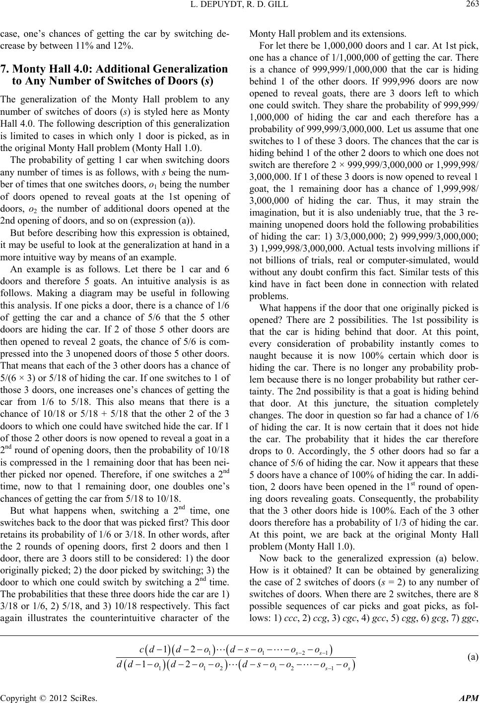

L. DEPUYDT, R. D. GILL
263
r of Switches of Doors (s)
hance of 5/6 is com-
pressed into the 3 unopened doors of those 5 other doors.
re
the door
ori
does not
sw
kind have in fact been done in connection with related
problems.
What happens if the door that one originally picked is
opened? There are 2 possibilities. The 1st possibility is
that the car is hiding behind that door. At this point,
every consideration of probability instantly comes to
naught because it is now 100% certain which door is
hiding the car. There is no longer any probability prob-
lem because there is no longer probability but rather cer-
tainty. The 2nd possibility is that a goat is hiding behind
that door. At this juncture, the situation completely
changes. The door in question so far had a chance of 1/6
of hiding the car. It is now certain that it does not hide
the car. The probability that it hides the car therefore
drops to 0. Accordingly, the 5 other doors had so far a
chance of 5/6 of hiding the car. Now it appears that these
5 doors have a chance of 100% of hiding the car. In addi-
tion, 2 doors have been opened in the 1st round of open-
ing doors revealing goats. Consequently, the probability
that the 3 other doors hide is 100%. Each of the 3 other
doors therefore has a probability of 1/3 of hiding the car.
At this point, we are back at the original Monty Hall
problem (Monty Hall 1.0).
Now back to the generalized expression (a) below.
How is it obtained? It can be obtained by generalizing
the case of 2 switches of doors (s = 2) to any number of
switches of doors. When there are 2 switches, there are 8
possible sequences of car picks and goat picks, as fol-
lows: 1) ccc, 2) ccg, 3) cgc, 4) gcc, 5) cgg, 6) gcg, 7) ggc,
case, one’s chances of getting the car by switching de-
crease by between 11% and 12%.
7. Monty Hall 4.0: Additional Generalization
to Any Numbe
The generalization of the Monty Hall problem to any
number of switches of doors (s) is styled here as Monty
Hall 4.0. The following description of this generalization
is limited to cases in which only 1 door is picked, as in
the original Monty Hall problem (Monty Hall 1.0).
The probability of getting 1 car when switching doors
any number of times is as follows, with s being the num-
ber of times that one switches doors, o1 being the number
of doors opened to reveal goats at the 1st opening of
doors, o2 the number of additional doors opened at the
2nd opening of doors, and so on (expression (a)).
But before describing how this expression is obtained,
it may be useful to look at the generalization at hand in a
more intuitive way by means of an example.
An example is as follows. Let there be 1 car and 6
doors and therefore 5 goats. An intuitive analysis is as
follows. Making a diagram may be useful in following
this analysis. If one picks a door, there is a chance of 1/6
of getting the car and a chance of 5/6 that the 5 other
doors are hiding the car. If 2 of those 5 other doors are
then opened to reveal 2 goats, the c
That means that each of the 3 other doors has a chance of
5/(6 × 3) or 5/18 of hiding the car. If one switches to 1 of
those 3 doors, one increases one’s chances of getting the
car from 1/6 to 5/18. This also means that there is a
chance of 10/18 or 5/18 + 5/18 that the other 2 of the 3
doors to which one could have switched hide the car. If 1
of those 2 other doors is now opened to reveal a goat in a
2nd round of opening doors, then the probability of 10/18
is compressed in the 1 remaining door that has been nei-
ther picked nor opened. Therefore, if one switches a 2nd
time, now to that 1 remaining door, one doubles one’s
chances of getting the car from 5/18 to 10/18.
But what happens when, switching a 2nd time, one
switches back to the door that was picked first? This door
tains its probability of 1/6 or 3/18. In other words, after
the 2 rounds of opening doors, first 2 doors and then 1
door, there are 3 doors still to be considered: 1)
ginally picked; 2) the door picked by switching; 3) the
door to which one could switch by switching a 2nd time.
The probabilities that these three doors hide the car are 1)
3/18 or 1/6, 2) 5/18, and 3) 10/18 respectively. This fact
again illustrates the counterintuitive character of the
Monty Hall problem and its extensions.
For let there be 1,000,000 doors and 1 car. At 1st pick,
one has a chance of 1/1,000,000 of getting the car. There
is a chance of 999,999/1,000,000 that the car is hiding
behind 1 of the other doors. If 999,996 doors are now
opened to reveal goats, there are 3 doors left to which
one could switch. They share the probability of 999,999/
1,000,000 of hiding the car and each therefore has a
probability of 999,999/3,000,000. Let us assume that one
switches to 1 of these 3 doors. The chances that the car is
hiding behind 1 of the other 2 doors to which one
 
itch are therefore 2 × 999,999/3,000,000 or 1,999,998/
3,000,000. If 1 of these 3 doors is now opened to reveal 1
goat, the 1 remaining door has a chance of 1,999,998/
3,000,000 of hiding the car. Thus, it may strain the
imagination, but it is also undeniably true, that the 3 re-
maining unopened doors hold the following probabilities
of hiding the car: 1) 3/3,000,000; 2) 999,999/3,000,000;
3) 1,999,998/3,000,000. Actual tests involving millions if
not billions of trials, real or computer-simulated, would
without any doubt confirm this fact. Similar tests of this


  
1
112
12
12
121
121
ss
s
s
s ooo
ds oooo



 


(a)
cddo d
ddodo o

 



L. DEPUYDT, R. D. GILL
264
and 8) ggg. The corresponding probabilities of the 8 se-
quences are as follows:
1)
112
12
12
cc c
ddo doo


 
2) 12
112
1
12
g
oocc
ddo doo


 
3) 2
112
1
12
gocc
ddo doo


 
4)
112
1
12
gc c
dd odoo


 
5) 112
112
1
12
g
og ooc
ddo doo


 
6) 12
112
1
12
g
oogc
dd odoo
 

 
7) 1
112
1
12
gogc
dd odoo


 
8) 112
112
12
12
g
og oog 

ddo doo 
The desired outcome, getting a car after two switches

n sequences 1), 3), 4), and 7). The
probability of getting a car after two switches of doors is
therefore the sum of the 4 probabilities 1), 3), 4), and 7).
The common denominator of this probability is as fol-

12
2do o  (b)
sams s and 1 therefore
of doors, is achieved i
lows.

1
1ddo
And e a considering that 2 is the
the same as 1
s
, this expression can be rewritten as
follows.



11
1
s
ss
dd sodoo



 (c)
), oe can derive the fol-
number of switches
(s).
  

112123
2 1
12 3
ss
dodo odooo
o o

 


(d)
as (e), without too
been so abbreviated
in expression (a) anticipated above.


112
1
12
s
By n
iny
extending both (b) and (c
lowg expression applying to an


123
123 1
1
ss
ds ooo
dsoo ooo

 


 


Expression (d) can be abbreviated
great loss of transparency, and it has
d

12
s
s
ddodo o
o o

 
 (e)
ility at hand is the fol-
sequences 1), 3), 4), and
7) above.
dsoo  
numerator of the probab
lowing sum of 4 terms found in

The



 

1
1
12 1
11
ccccg oc
gc cggoc

 

This sum can be rewritten as follows.





 

1
1
12 11
1
cccccg occg
cg go
 

And therefore also in successive steps as follows.














 
 
 

11
11
11
11
1
1
1
12 111
12 11
12 2
122
12
12
12
ccccgoc gggo
cccgo gcgo
cccg ogcgo
ccdo gdo
cc gdo
cc gdo
cd do
 




 

  



  

 

(f)
And considering that 2 is the same as s and 1 therefore
the same as 1
s

, expression (f) can be rewritten as fol-
lows.




1
1s cdsds o

 
 (g)
By extending (f) and (g), one can derive the following
expression of the numerato
switches (s).
r applying to any number of








112
123 2
122 1
123
1ss
ss
cddo do o
dsoooo
dsooo o


 
 




 


(h)
Expression (h) can be abbreviated as (i), without too
great loss of transparency, and it has been so abbreviated
in expression (a) anticipated above.



 
112
121
12 3
ss
cddo do o
dsoo o

 
  (i)
In the specific

case of the above example featuri
car, 6 doors, and 2 switches of doors, the gene
si
ng 1
ral expres-
on assumes the following form.




 
1
12cddo
11 2
12dd odo o 
Entering the relevant integers, one obtains the prob-
ability already given above.




 
16162210  
’s chances of get-
ting a car after s switches is therefore as follows.
6 6126221 18 
The chances of getting a car at the first door pick is c/d.
The factor by which one increases one

L. DEPUYDT, R. D. GILL 265
 


   
1
2121
12
ss
112 1
1
12
s
s
dd s
dod d
 
 
g a car from 1 switch to s switches is therefore the following.
od
oo

 


o oo
soo oo


 


The factor by which one increases one’s chances of gettin
 


  
112
23 121
1212312 1
23
ss
s
s
dso oo
doodooodsoo oo






Finally, in Monty Hall 3.0, when more than 1 door is
pi re are 2
ru oq. Doors are
switched only 1 time (s = 1). If more than 1 d or is
picked at each pick and doors are switched more than 1
tim
fr
8. Back to Boole. By Richard D. Gill
8.1. Summary
I comment on Leo Depuydt’s recent work on applying
Boole’s work in probability theory to the Monty Hall
problem. In particular, I compare Boole’s notation and
conventional modern probability notation, discuss mod-
ern computational tools, and make some comments on
Boole’s position that probability theory belongs to the
laws of thought.
oole’s work on probability theory stands on an
equal intellectual level to his work on l
tended by him to be seen as an integral p
has largely been forgotten. Now that three half centuries
have gone by and probability theory has flourished, fol-
lowing different routes, his work is harder than ever to
re
find his way into Boole’s way of thinking.
In this paper and its predecessor Leo tackles a number
of variants of the Monty Hall problem, showing how
oole’s approach leads to solutions despite ever increase-
ists. I emphasize
ilists con-
one could better say, ill posed.
laim, influential writers of the early
as
dependence should
be assumed. In modern day terms, Boole fitted judiciously
chosen log linear models to the data, judicious
higher order interactions about which there was no in-
fo
are represented by
graphs and the same graphs used as fdation for
graph-theoretic based computations.
However, I do not know if Depuydt is also going to
“a
Boole indeed saw probability theory as part of the laws
of thought. His probabilities are subjective degrees of
belief, their numerical values follow logically from con-
si
of in-
difference, but using indifference not just to specify
probabilities but also to specify probability structures.
However, so far, we are considering here problems
where all probabilities are completely specified and
where a frequentist (objectivist) and a Bayesian (subject-
force unique values of probabilities from “equally likely,
by symmetry” arguments.
rn day notation by means of a simple
(mathematical) example. Consider four events which can
sequence. For instance, the results
dodoo 
cked both before and after doors are opened, the
ns of coefficients, 1 for p and 1 fr
o
e, there will be more than 2 coefficients. I refrain
om entering into detail at this time.
8.2. Introduction
George B
ogic, and was in-
art thereof, yet it
ad. It is impressive that Leo Depuydt has been able to tivist) approach will give the same probability values,
since in either approach the symmetries of the problem
B
ing complexity. From the point of view of a present day
professional mathematician, my first questions were: are
the answers correct? Is Boole’s probability different from
present day probability?
The answers so far are yes: the answers are correct, and
no, Boole (and with him Depuydt) is using the same
probability rules as present day probabil
so far because Boole also claimed to be able to solve
probability problems which modern day probab
sider insoluble, or perhaps
Because of this c
twentieth century such as Keynes dismissed Boole’s work
completely, and that hastened its progress into limbo. As
Miller (2009) points out [9], however, Boole’s solution
was meaningful and complete, and based on adding an
8.3. Notation
It is easiest to explain the difference between Boole’s
notation and mode
sumption that in absence of further information, and in
particular, with no logical dependencies, an appropriate
higher level of conditional statistical in
ly dropping
rmation anyway. This connects to modern develop-
ments in graphical models (also known as Bayes nets),
another development which Boole would have appreci-
ated, in which probability models
oun
uthorize” this particular, more controversial part, of
Boole’s thinking.
deration of information (known and unknown). He stood
here full square in the nineteenth century tradition of
Laplace, deriving probabilities from the principle
occur, or not occur, in
of a first pick of a door, a second pick, and so on. Let me
denote the events as A, B, C, D (capital letters early in the
alphabet, according to present day conventions). The
modern view of probability theory is that we may consider
these events equally well as subsets of a set

“ele-
mentary outcomes.” The event A is identified with the set
of all elementary outcomes

 for which A does
indeed happen. Probabilities are assigned to subsets of

,
and set theoretic operations turn out to correspond to
g events. For example, the logical constructions involvin

L. DEPUYDT, R. D. GILL
266
event that both A and B occur corresponds to the outcome
of the probability experiment,

 , being both a
member of the subset A and the subset B. Thus the prob-
ability of A and B happening is identified with


PA B,
where

P is a mapping from subsets of  to numbers
between zero and one.
Subsets A, B, etc., are often called “compound events.”
Provided however we are careful with language, the
words “elementary” and “compound” in the two contexts
“elementary outcomes

 ” and “compound events
A,” are superfluous. But it also does no harm to add
them. The elementary outcomes correspond to the most
fine-grained, most detailed, description of what actually
happened. Compound events correspond to coarse-
grained descriptions, by which many alternative “micro-
scopic” ways according to which the same “macroscopic”
phenomenon can come about are all grouped together.
Whatever probabilities are supposed to mean (whether
relative frequencies in the long run of many repetitions, or
whether degrees of belief as measured by fair betting
odds), everyone agrees that if two events can never hap-
pen together, the probability that either occurs is equal to
the sum of their probabilities; that certainty corresponds
with probability one; and that all probabilities are greater
than or equal to zero. Converting these minimal properties
into the language of set theory, we obtain the now familiar
axioms:

1P,

0PA for all A,
AB implies
 
PA BPAPB . Finally
we add as a definition of conditional probability of A
given B, as long as

0PB:


P
ABP ABP B .
From these minimal properties one can derive the fol-
lowing chain rule:

 
and and and
andand and.
PA B CD
PAPBAPCA BPDA BC (1)
However, the alert reader will have noticed that I am
mixing the language of logic and the language of ele-
mentary set theory in this equation, and I do that deliber-
ately, in order to point out an important ambiguity in the
translation from logic to set theory.
The interpretation of the left hand side is obvious: I
could have written (should have written!), of course,

PA BCD . The right hand side certainly makes
sense, and indeed the statement is true, if I do the corre-
on that side; for instance, the last sponding substitutions
term should be

A C. However there is an
Let me explain. Suppose start with a probability
PD B
I
alternative substitution, more clumsily expressed in set
theoretic language, but equally meaningful from the point
of view of natural language. The correctness of this al-
ternative interpretation is actually a theorem.
measure P. Next I pick some event B with positive prob-
ability, and compute new probabilities



B
PA PAB
for every event A.
Theorem 1: the conditional probability measure A P
also satisfies the axioms of probability theory;
Theorem 2 (principle of repeated conditioning):

B
AAB
PP

.
This is not just empty formalism, it tells us something
very important: conditioning in turn on any number of
events gives end results which do not depend on the order
in which we take them, and is not changed by
grouping them into a smaller number of events by using
the rule P(A|B and C) =
also


P
AB C. It shows ue
transition between the language of logic and the language
of sets is very smooth indeed
s that th
.
For B
does fi
Boole has no use for the language of sets. It was not
even yet invented: his supporter and contemporary John
Venn was one of those who pioneered its use; indeed, its
use in probability theory.oole, the language of logic
ne both for events and for probabilities of events.
Defining the event E as “A and B and C and D,” Boole
writes the definition of the event E as


logical relatione abcd, (2)
and then rewrites Equation (1), a relation between prob-
abilities and conditional probabilities, with the very same
sequence of symbols:


numerical relation between probabilitieseabcd, (3)
Even though Equation (3) is to be interpreted numeri-
cally as a relation between probabilities, the rules of al-
gebra have to be handled with very great care. The exact
sequence of probabilities abcd corresponds to a specified
sequence of events A, B, C, D and there is a logic to this
sequence: typically this will be their temporal ordering.
The valud tomerical ve c, f
n front of
events a and b. Event D might be certain in some context,
impossible in other. Tced
e assigne the nuariablor in-
stance, depends on the context, on the presence i
he preing events A, B and C
could switch the probability d to 1, or to 0. This is what
Depuydt calls the digital nature of probabilities.
One of the fruits of the digital revolution has been statis-
tical computing and computer algebra. Looking at
huge tables of probabilities in sections 4.1 and 4.17,
reader may worry that perhaps some typesetting error has
co
nother opportunity
fo
8.4. Computations
the
the
rrupted one of the formulae. If the reader actually
wanted to use those formulae to do numerical computa-
tions, he or she might want a computer do those compu-
tations. But then the typeset symbols have to be translated
into lines of computer code, which is a
r errors to creep in.

L. DEPUYDT, R. D. GILL 267
I have verified that it is in principle possible to repro-
sing computer algebra. Let the com-
puter do the painstaking, repetitive task of applying sim-
ple rules of transformations of formulas! Let the computer
typeset the page let the computer also
generate computer code for implementation to specific
cases! Then the reader need only check the programs or
scripts: do they implement Boole’s logic of probability?
There are two levels involved here. The prob
duce these tables u
s in the journal,
lem should
be
ich the computer
ows. Anyone who understands the
la m
must be
ch day
for a myriad asks also provide external consistency
checks whene answer can be got by different
m
Sage (http:
publicly available, and
an
orithms which it
uses are public; the scientist can check th
them by new algorithms of their own.
of a particular generalized Monty
Hall problem, count outcomes of different kinds, in o
to statistically estimate the probabilities which can in
pri
as cer-
a short time Sage has become
flexible. Like natural languages,
e of ball-picking in phase one.
culture, and like mathematics itself, these systems evolve
through highly effective “crowd-sourcing.”
8.5. Alternative Approach
Depuydt goes back to first principles and determines the
probabilities of all possible elementary outcomes of his
Monty Hall games: any particular sequence of picks of
doors. Now, it is possible to group some of the picks to-
gether, producing a coarser level of description, but one in
w
described in a high level formal language which
translates line by line Depuydt’s verbal descriptions of
what he is doing into a language wh
algebra system kn
hich (a) the components of the coarser description cor-
respond to familiar probability models, and (b) the coarser
description is fine enough to still allow specification of the
compound events of interest.
In Monty Hall 3.0, such a coarser description is possible
at the level of phases. Recall that in this game, c doors
hide cars, g doors hide goats, d = c + g is the total number
of doors. The player first picks p doors. The host then
opens q doors, revealing goats. The player may now
switch to another r doors.
The hosts’ possibilities are delimited by how many cars
are hidden by the player’s first p picks. Call this number x.
We can now write down the joint probability of x cars
being behind the player’s first p picks, and y cars being
behind the player’s second r picks, as follows. Both
phases correspond to a traditional “sampling without
replacement” situation, picking balls from vases, where
the composition of the vase at phase two is determined by
the outcom
nguage can verify that it is “the same thing.” The i-
plementation of the computer algebra system
ecked by specialists, though users who use it day by
of t
ver the
eans.
I would like especially to draw the reader’s attention to
two powerful tools, both of them completely free (both in
the sense of “free beer” and in the sense of “free speech”):
the statistical language R (http://R-project.org) and the
computer algebra system//sagemath.org). The
freedom as in free speech is the fact that the computer
code of both R and Sage itself are
yone is allowed not only to look at it but also to modify
it, repackage it, and even to sell it, as long as their modi-
fications preserve the same freedoms.
Sage allows one to instruct the computer to perform
algebraic formula manipulations according to specified
rules. Boole would have appreciated that. Unlike com-
mercial tools like Mathematica, the alg
Suppose a vase contains R red balls and B blue balls, let
N = R + B be the total number of balls in the vase. Sup-
pose n balls are picked at random from vase, without
replacement, and completely at random. Define the bi-
nomial coefficient

!! !
n
x
Cnxnx, the number of
ways to choose x objects from a collection of n. In spoken
mathematics, one says “n choose x” instead of “C super-
script n subscript x.” Let r be the number of red balls in the
sample of n, and define bnr to be the number of
blue balls. It turns out that the probabilit
em, even replace
R is a statistical computing tool. One thing which is
extremely easy with R is to run a computer simulation of
millions of repetitions
y to find exactly r
re
rder
d balls is h(r; n, R, N) =
R
BN
rbn
CCC. The fact that these
so-called hypergeometric probabilities must add up to one
as one adds over all possible values of r is called the
Chu-Vandermonde identity in combinatorics, going back
to Chu Shi-Chieh, 1303, and Alexandre-Théophile Van-
dermonde, 1772. One can say that Depu
nciple be computed algebraically.
Both these systems are widely used in academia, in
teaching, in industry; they have huge followings and be-
cause of their open nature, additions have been written
by users from all kinds of application fields which any-
one else can also freely use. The user communities with
their internet fora and mailing lists and so on, allow both
the new user and the expert to get advice from fellow
users all over the world, often extremely rapidly and ef-
fectively. R can even be used from Sage—one of the
design philosophies of Sage is to use existing tools, so as
not to waste time re-engineering wheels. This h
ydt has derived a
“two-level” generalization of this identity from first prin-
ciples, following Boole’s methodology.
Now if among the first p doors chosen by the player
exactly x doors hide cars, then at the second stage, when
there are dpq

 doors left from which the player may
choose r doors, a further q doors already having been
op
tainly paid off, since in
extremely powerful and
ened revealing goats, exactly cx  of those doors hide
cars, and


g
px q

hide goats. This tells us that the
probability that the player’s first p picks hide x cars and

L. DEPUYDT, R. D. GILL
268
his second r picks hide y cars is
 
;,,;,,hxpcdhyrcxdp q.
This gives an alternative way to check the results of
this paper.
9. Empirical Definition of Mathematics, in
Boole’s Footsteps, as a Cognitive Event on
the Deepest Level
9.1. Where Is Mathematics?
The question that is at the center of the present section is
as follows: What is mathematics? The answer to this
iderable interest. No endeavor of the
cessful. Evidently, the
een basically two diametric-
mathematics
e may interpre
inside t
ught to co
said about that
ca
rally, number
when it comes to em-
pirical observation, numbers can ly be observed and
th
ing to the brain. Mathematics is something
that the brain does.
9.2
This to pursue a line of inquiry
a half ago but fairly
question is of cons
ca
ca
ca
human intellect has been more suc
question has occupied many, many minds over the centu-
ries. The literature on the subject is massive. But even
the most cursory review of what has been done readily
reveals that the question can hardly be considered an-
swered. There has been no lack of attempts to provide an
answer. However, the proposed answers seem often ir-
reconcilable and can even be diametrically opposed.
In order to define mathematics, one needs to be able to
observe it. A second question therefore presents itself, as
follows: Where is mathematics? In other words, where
n one find mathematics so that one can take a look at it
and analyze it in order to determine what it really is?
It appears that the answer to the seemingly simple
question as to where mathematics is has perhaps been the
greatest point of controversy in the discussion of what
mathematics is. There have b
lly opposed answers to the question where mathemat-
ics is. Some believe that mathematics is something inside
the head. Others believe that it is something outside the
head. Whereas many believe with Kurt Gödel that num-
bers exist independently of the human mind, many others
like L.E.J. Brouwer are convinced that numbers are a
creation of the human mind. Could both be right at the
same time?
The position that I will adhere to is that
n only be empirically observed as something that is
inside the head. This position in no way involves a denial
of the notion that mathematics is something outside the
head. Clearly, when applied to reality outside the head,
mathematics works. Somt this as proof that
mathematics is also something outside the head. Then
again, the totality of human experience of reality outside
the head is how the brain perceives and processes this
reality through the senses he head. This percep-
tion is itself 100% brain activity. Therefore, the analysis
of the human experience onsist in the final re-
sort, on the deepest level, of the analysis of brain activity.
And one component of the brain activity that constitutes
the human experience is mathematics. In that regard, the
question as to whether mathematics is also something
outside the brain is to some extent moot because mathe-
matics cannot be empirically observed in that capacity
anyhow, so there is hardly anything to be
pacity.
To some extent, Gödel’s position and Brouwer’s posi-
tion are not in opposition. There is nothing that contra-
dicts the notion that numbers are something that is both
something outside the head and something inside the
head. Natus would inhabit different medi-
ums inside the head and outside the head, physical reality
and brain mass respectively. But
on
erefore also analyzed as an activity of the brain or an
event happen
. Resuming an Abandoned Line of Inquiry
e aim of what follows
that was initiated about a century and
soon completely abandoned and ever since entirely dis-
regarded. This line of inquiry is, I believe, worthy of be-
ing resumed. It appears to me that it can lead to a final
definition of mathematics and its foundations. The ini-
tiator of the line of inquiry in question was George Boole,
first in his The Mathematical Analysis of Logic (1847)
[13-16], but then above all in his An Investigation of the
Laws of Thought (1854), which may be regarded as the
Magna Charta of the digital age [17,18]. The principal
follower of Boole was John Venn in his Symbolic Logic
(second edition, 1894) [19]. Whitehead notes that Venn
gave “thorough consistency to Boole’s ideas and notation,
with the slightest possible change” [20] and, more re-
cently, Styazkhin observed that Venn “revealed the es-
sence of the secret of success of Boole’s procedures”
[21].
The Digital Age owes an extraordinary debt to Boole
and to the digital mathematics that he created. Digital
mathematics is a type of mathematics that is distinct from
the more familiar type of mathematics, quantitative
mathematics (to which Boole also made significant con-
tributions, for example by his work on differential Equa-
tions). But digital mathematics is in the end just as
mathematical as quantitative mathematics. Clearly, a line
of inquiry initiated by Boole has proved to be successful.
Little did Boole know to which uses his digital mathe-
matics would be put when he wrote in 1847, “It would be
premature to speak of the value which this method may
possess as an instrument of scientific investigation” [22].
9.3. Probability Theory as an Ulterior Aim of
Said Line of Inquiry
It is not clear to which extent Boole, when initiating the
line of inquiry that ultimately spawned the Digital Age,

L. DEPUYDT, R. D. GILL 269
had something like computer science in mind as an ulte-
rior aim. In fact, in his Laws of Thought, digital mathe-
matics is clearly subordinated to an ulterior aim of an
entirely different kind, namely making classical prob-
ability theory complete.
It is not entirely certain whether Boole had this rela-
tion of subordination to probability theory in mind as
soon as he began working on digital mathematics. There
is no mention of probability theory in his The Mathe-
matical Analysis of Logic of 1847, in which he first es-
tablished his digital mathematics. But in Laws of Thought,
digital mathematics is clearly styled as serving the aims
of probability theory, as appears from the second part of
the book’s long title, (An Investigation of the Laws of
Th
ght and Language as an
Ulterior Aim of Said Line of Inquiry
of
Boole’s Work on Logic and Probability
Boole of giving his 1854 book the wrong title. He be-
dealght,” because “the question
reflec-
g
the p
cates with another through thought and
la
same
ought), on Which Are Founded the Mathematical
Theories of Logic and Probabilities.
A great irony relating to Boole’s legacy is that his
work on probability theory has been, with one or two
exceptions [23], completely disregarded, almost entirely
bypassed by the field. In the planned article mentioned at
the end of §1, I intend to confirm that Boole’s probability
theory does what it claims to do, make classical probabil-
ity theory complete, and how it does so.
9.4. Rational Thou
But there seems to be more to the ulterior aims
Boole’s digital mathematics than statements about prob-
ability theory. Boole’s Laws of Thought and many of his
other works on logic and probability, both published and
unpublished, are replete with references to the nature of
human thought in as far as thought is rational. The ques-
tion as to whether he aimed to determine what is going
on in one’s head when one thinks rationally is investi-
gated below.
In any event, like Boole’s ideas on probability theory,
this component too of his line of inquiry appears to have
fallen by the wayside. Whereas the forthcoming article
mentioned at the end of §1 is an attempt to validate
Boole’s line of inquiry in relation to probability theory,
what follows is an attempt to resume and extend this
same line of inquiry as it relates to the deepest founda-
tions of rational human thought and mathematics.
9.5. Is
Mathematical or Cognitive in Nature?
9.5.1. Modern Perception of Boole’s Work on Logic as
Strictly Mathematical
When one reads Boole’s writings on logic and probabil-
ity, the following question easily arises: Is Boole doing
mathematics or is he trying to determine how people
think rationally? In other words, is he describing the
mathematical structure of reality or is he trying to tell us
what is going on in people’s heads when they think ra-
tionally? Boole’s contributions, to the extent that they
have proved lasting, are now universally perceived as
belonging to the realm of mathematics. Boolean algebra
is after all ubiquitous. Bertrand Russell even accused
lieved that Boole was “mistaken in supposing that he was
ing with the laws of thou
how people actually think was quite irrelevant to him”
[24-26]. Taking into consideration how people think
while practicing mathematics is sometimes called psy-
chologism, which some seem to regard as a bad word.
9.5.2. Statements to the Contrary in Boole’s Writings
There are abundant indications in Boole’s work that
leave no doubt that how people think, at least as far as
rational thought and language is concerned, was very
much on his mind. In the Preface to the earlier Mathe-
matical Analysis of Logic (1847), he states that he is not
concerned with “quantity,” but with “facts of another
order which have their abode in the constitution of the
Mind” [27]. In the first statement following the Preface
to the later Laws of Thought (1854), he announces [28]:
“The design of the following treatise is to investigate
the fundamental laws of those operations of the mind by
which reasoning is performed.”
How can such statements, when taken at face value,
not pertain to what is going on inside the heads of people
—notwithstanding attempts to soften their impact, per-
haps to protect Boole from the charge of psychologism?
[29].
Two possible reasons for resisting the notion that
Boole could have been aiming to establish how the brain
works are as follows.
First, mixing Boole’s mathematical results with
tions on the nature of thought might be seen as affectin
urity and objectivity of the former.
Second, at the present time, it remains still basically
unknown—let alone that it was in Boole’s time—how
the brain produces rational thought and language in bio-
chemical terms, that is, which activities of neurons and
synapses are responsible. So how could anyone have
anything to say about how the biological brain reasons?
The first objection is addressed below. In regard to the
second objection, I have noted elsewhere that, as one
brain communi
nguage, all communications need to travel by air from
the mouth of a speaker to the ear of a hearer or by light
from the written page to a reader’s eyes. There can be no
doubt that everything that is essential to the structure of
rational thought and language must be conveyed in sound
waves or light beams that travel from mouth to ear or
from page to eye. In that sense, the structure of rational
thought and language is empirically accessible. The

L. DEPUYDT, R. D. GILL
270
structure ought to be present inside the brain, even if
ting a different medium.
in-
habi
sa
is a good illustration of
this definition. It seems otherwise quite tempting to in-
a
prope e the brain. As it happens, that
the Brain
d in the end avoid
de
ite of this assumption is that there is something
more to reality than what is perceived through the senses.
uld be.
Relig ut that something
9.5.3. Boole’s Own Perception of His Work on Logic
as Mathemati cal
While there can be no doubt that how the brain thinks is
somehow a prominent concern in Boole’s writings, there
are also plenty of statements in his writings that leave no
doubt that he is firmly convinced that what he is doing
when he is studying logic and probability is mathematics.
He states, for example, that “the ultimate laws of Logic
are mathematical in their form” [30].
As one tries to assess what exactly it is that Boole is
trying to do, the impression gradually imposes itself and
becomes inescapable that he is writing both about how
the mind thinks and about mathematics. There are just
too many categorical statements in his work that posi-
tively point to both. At this juncture, there is the possibil-
ity of assuming that there is something deeply confusing
and contradictory in Boole’s work. One might seek to
resolve the possible contradiction by discarding either the
cognitive facet or the mathematical facet of Boole’s work
as invalid. In choosing to reject either of the two, the
easier choice would seem to be the cognitive facet. The
mathematical facet has more than proved itself by appli-
cations in modern computer science.
Then again, it is difficult to overlook the many pas-
sages that concern how the mind thinks. Consider his
analysis of the syllogism, which does not supplant Aris-
totle’s analysis but rather completes it. It seems easy for
all to agree that we must think according to the rules of
the syllogism if we are to reason correctly. And more
generally, it is easy to convince oneself that what Boole
says about how the mind thinks rings true. There just
seems to be more to Boole’s writings than just mathe-
matics.
9.5.4. Could Boole’s Work on Logic Be Both
Mathematical and Cognitive?
The question arises: Could Boole have been doing both
at the same time, producing mathematics and describing
mental faculties? The following statement by Boole
clearly indicates that his approach is at the same time
mathematical and cognitive. What he sets out to discover
is the mathematical structure of rational cognition [31]:
“The laws we have to examine are the laws of one of
the most important of our mental faculties. The mathe-
matics we have to construct are the mathematics of the
human intellect.”
The present discussion has reached a critical juncture.
It needs to be decided whether the cognitive facet of
Boole’s line of inquiry should be pursued or dropped
altogether. The validity of Boole’s digital mathematics
ys something about the overall soundness of his think-
ing. It can serve as an argument in favor of resuming the
cognitive facet of the same general line of inquiry.
In resuming the cognitive facet, the concept described
by Boole as the “mathematics of the human intellect”
cited above will serve as a point of departure. What can
possibly be meant by this concept? It would seem that it
places mathematics somehow inside the human intellect.
The way in which the concept will be interpreted in what
follows is that mathematics is in essence a property and
an activity of the brain. Mathematics is best defined as
something that the brain does. In a planned article, I hope
to show that probability theory
terpret mathematics as exactly the opposite, namely as
rty of reality outsid
very notion will also be assigned a place in the definition
of mathematics as something that the brain does. Mean-
while, the principal consideration that leads to the defini-
tion of mathematics as an activity of the brain is pre-
sented in the next section.
9.6. Mathematics as an Activity of
The brain is evidently the most complex structure in the
universe. It consists of billions of neurons and trillions of
synapses. Still, it seems just as evident that the brain is a
biological mass that is limited in size. There is only so
much of it and no more. The following working hypothe-
sis therefore seems to impose itself. The time will come
when it will be possible to record everything that the
brain does as it happens, presumably with the aid of su-
percomputers or the like. The opposite of this hypothesis
is that a certain part of the brain will be forever inacces-
sible. But what could such an inaccessible part consist of?
If everything in the brain is atoms and molecules and the
like, then no activity in the brain shoul
tection, one would think.
Another basic assumption is that the totality of human
existence as we know it consists of how the brain per-
ceives reality outside itself through the senses. There are
many more senses than the classic five, including sensing
the effects of the instincts with which the brain comes
equipped at birth. In addition, perceptions received
through the senses can be recombined in certain ways
inside the brain. Dreams are one type of recombination.
The oppos
It is difficult to see what that something more co
ion makes certain assumptions abo
more. But then, it is impossible to make everyone agree
on what that something more is and the assumptions of
religion are beyond scientific verification anyhow.
Once it is possible to record everything the brain does
in its entirety, part of what is recorded will be the brain’s

L. DEPUYDT, R. D. GILL 271
knowledge and practice of mathematics. It should be
po
rded brain activity?
r understanding. The brain
edge
form
g mathematics. It is an im-
po
rva-
tio
itself subject,
without its being also given to it to understand their
-
gree r fitness for their end, as com-
ssible to observe exactly what the brain does when it
engages in mathematics and how it starts up mathematic-
cal knowledge. The key question arises: Is there more to
mathematics than reco
9.7. The Brain as the Final Frontier: Towards a
New Empiricism
If the totality of the human experience consists of how
the brain engages what is outside itself, then nothing that
does not have some kind of imprint in the brain can mean
anything to the brain. In assessing what is outside itself,
the brain only has itself, as it were, to sort things out.
And by itself is meant a complex and very large but ul-
timately limited and fully definable amount of activity of
neurons and synapses and the like.
At first sight, it would seem as if mathematics is a
property of reality in which the brain occasionally par-
ticipates. Mathematics seems like a sacred code inscribed
in the book of nature. But all that the brain can ultimately
know about this code is the details of its own participa-
tion. And the details of this participation consist one
hundred percent of brain activity. Therefore, if one truly
wants to understand what mathematics is, then all one
has as an object of study is the participation itself as
brain activity. It is understandable that there may be a
desire for more than just that. But the brain can hardly
step outside itself, as it were. It is fully limited to its own
activity and powers, and to the study of this activity and
these powers in a search fo
activity does not only include mathematical knowl
and reasoning, but also the act of perception in the
of signals reaching the brain from outside through the
senses. Needless to say, once it is possible to observe all
this brain activity, it will also be possible for this very act
of observing brain activity to be itself observed, include-
ing by the person whose brain activity is being observed.
It is a bit like a snake biting its own tail.
But what about the ever attractive notion that mathe-
matics is a property of nature outside the brain? Nothing
is more tempting than to subscribe to this assumption. In
fact, I believe that there is nothing wrong with assuming
that reality exhibits a structure that may be called
mathematical and that this structure is somehow the ori-
gin of a certain type of brain activity that may be de-
scribed as knowing and doin
ssible to avoid assumption under which everyone ef-
fectively operates. One way of looking at the matter is as
follows. It is not because there is no final verification of
this assumption that the assumption should be rejected.
The assumption receives abundant support from the fact
that mathematics works. When mathematical knowledge
is acquired and this knowledge is then returned to reality
outside the brain by being applied correctly, as in build-
ing a bridge, the application will typically work, that is,
the bridge will not collapse. But ultimately, mathematics
can only be observed to the extent that it can be seen at
work in the brain. Reality is experienced entirely in terms
of how the brain engages what is outside itself through
the senses. The scientific observation and analysis of this
experience therefore ultimately needs to be the obse
n of the brain. And that also applies to mathematics as
one type of reality. Anything else is beyond human
knowledge. It is not possible to look behind the curtain,
as it were, to establish why the brain is the way it is.
Along these lines, Boole’s writes in somewhat Latinate
English, “It may, perhaps, be permitted to the mind to
attain a knowledge of the laws to which it is
ground and origin, or even, except in a very limited de
, to comprehend thei
pared with other and conceivable systems of law” [32].
Because the assumption that the structure of reality
outside the brain is mathematical is just an assumption, it
is not possible to probe the deeper roots of this presumed
structure. There is of course nothing that prevents anyone
from engaging in speculation to any degree. It is likewise
possible to speculate without restrictions about other
possible types of realities in which other possible types
of mathematics apply.
Knowledge is ultimately a process of assimilation in
which the brain assimilates to reality outside itself. For
example, to find one’s way through the streets of a city
without consulting a street map, the brain needs to ac-
quire something of the structure of the layout of the
city’s streets and in that sense become a little like that
layout. But it is reasonable to assume that, in the process
of assimilation, there needs to be something to assimilate
to. Therefore, if part of the assimilation is mathematical,
there is presumably something mathematical in reality
outside the brain to which the brain assimilates.
The fact that the knowledge of mathematics is stored
in the books of a mathematics library may also seem to
suggest that mathematics is something outside the head
and hence first and foremost a property of nature, with its
reflection inside the head being somehow secondary.
However, the books in question are nothing more than
paper and ink until an active brain reads and studies them.
In that sense, a tree does not fall in the forest if there is
no one there to hear it. The mathematics in a book is not
mathematics if it is not actively engaged by a thinking
brain.
9.8. Conclusion
It is possible to reconcile as complimentary the view ad-
hered to by someone like Brouwer that mathematics is

L. DEPUYDT, R. D. GILL
272
something inside the head and the view adhered to by
someone like Gödel that mathematics is something out-
side the head. In other words, the two views do not con-
tradict one another. However, that mathematics is some-
thing outside the head is only an assumption. But it is an
assumption that is hard to deny. So to some degree
Gödel’s view can be recognized. Still, it is only as some-
thing inside the head that mathematics can be truly ob-
served and therefore become the subject of empirical
inquiry once the secrets of the brain are unlocked. In that
regard, the cognitive approach is the only one that offers
a systematic path of scientific investigation. I hope to
apply the cognitive approach in planned papers, begin-
ning with the branch of mathematics called probability
theory. It will be useful to formulate the foundations of
probability theory fully in cognitive fashion.
10. Acknowledgements
When the present article was essentially complete, a for-
tunate set of circumstances brought the author in contact
with Dr. Richard D. Gill, Professor of Mathematical Sta-
tistics at the Mathematisch Instituut of Leiden University
in the Netherlands, who has contributed a number of
studies to the analysis of the Monty Hall problem. An
interesting exchange of ideas ensued about all sorts of
facets of the expanded Monty Hall problem and about the
contents of the present article. I personally profited much
from this exchange. One result of the exchange was the
decision to include, for the benefit of a somewhat more
interdisciplinary audience, an appendix by Professor Gill
(see §8). The design of this appendix is to provide addi-
tional context by building a bridge to modern probability
theory in its conventional notation and by pointing to the
benefits of certain interesting and relevant tools of com-
putation now available on the Internet. A more detailed
and in-depth description of the common concept of the
hypergeometric distribution in its relation to the contents
of the present article remains desirable and will need to
be postponed to future papers. The present collaboration
is meant as a first step conceived and executed on short
notice, an exploratory effort that probes what is possible
in terms of interdisciplinary projects spanning both the
humanities and the sciences. I am grateful to Professor
Gill for his willingness to make this much appreciated
contribution.
As regards the interdisciplinary nature of the larger
project of whose mathematical branch this article is part,
one ulterior aim is to promote the perfect unity of nota-
tion of Boole’s algebra and the complete unity of human
intelligence that it suggests, in that the notation can be
applied to the following multiple facets of human intelli-
gence, each illustrated here by one expression.
1) “The sun shines” (Language, Level of the Things).
2) “When the sun shines, I go to the beach.” (Lan-
guage, Level of the Events).
3) “Humans are mortal. Socrates is a human being.
Therefore, Socrates is mortal.” (Logic, but not just with
three statements, as in the present example, but with any
number of statements).
4) A quadratic equation (Quantitative mathematics).
all problem (Digital mathematics, in 5) The Monty H
addition to quantitative mathematics).
Finally, I also thank Dr. Michael R. Powers, now Pro-
fessor of Risk and Insurance Mathematics at Tsinghua
University in Beijing, China, for his continued interest in
the subject matter of this article and for fruitful discus-
sions in this connection about the essence of probability
in both its strictly mathematical and its more subjective
interpretations.
REFERENCES
[1] L. Depuydt, “The Monty Hall Problem and Beyond:
Digital-Mathematical and Cognitive Analysis in Boole’s
Algebra, Including an Extension and Generalization to
Related Cases,” Advances in Pure Mathematics, Vol. 1,
No. 4, 2011, pp. 136-154. doi:10.4236/apm.2011.14027
[2] Cf. J. Rosenhouse, “The Monty Hall Problem,” Oxford
University Press, Oxford and New York, 2009 (history of
the problem and its context).
[3] Cf. R. Deaves, “The Monty Hall Problem: Beyond Closed
vidence of the interest in the Doors,” 2006 (additional e
problem). www.lulu.com
[4] Cf. M. vos Savant, “Q(uestion) & A(nswer) (involving
the Monty Hall Problem),” Parade, 9 September 1990
(article serving as principal catalyst of the interest in the
problem).
[5] H. H. Goldstine, “The Computer from Pascal to von
Neumann,” Princeton University Press, Princeton, 1972,
p. 37.
[6] L. Depuydt, “The Monty Hall Problem and beyond:
Digital-Mathematical and Cognitive Analysis in Boole’s
Algebra, Including an Extension and Generalization to
Related Cases,” Advances in Pure Mathematics, Vol. 1,
No. 4, 2011, pp. 135-154, at p. 148.
[7] A. W. F. Edwards, “Pascal’s Arithmetical Triangle: The
Story of a Mathematical Idea,” Johns Hopkins University
Press, Baltimore, 2002, p. xiii.
[8] L. Depuydt, “The Monty Hall Problem and Beyond:
Digital-Mathematical and Cognitive Analysis in Boole’s
Algebra, Including an Extension and Generalization to
Related Cases,” Advances in Pure Mathematics, Vol. 1,
No. 4, 2011, pp. 135-154, at p. 145.
[9] L. Euler, “Elements of Algebra,” Springer Verlag, New
York, Berlin, Heidelberg, and Tokyo, 1984, pp. 110-120.
[10] S. F. Lacroix, “Traité élémentaire du calcul des prob-
abilités,” Fourth Edition, Mallet-Bachelier, Paris, 1864, p.
30.
[11] L. Depuydt, “The Monty Hall Problem and Beyond:

L. DEPUYDT, R. D. GILL
273
[1
ed in what follows).
[1
sa, Boole’s “×” (AND) is electrical
”
Investigation of the Laws of Thought, on
athematical Theories of Logic
and Probabilities,” Walton and Maberly, London, 1854.
[18] I have used thover Publications,
ass., 1969, p. 214.
ell, Vol. 3,” Routledge, London, 1993, pp. 366-379.
.
iv.
ic
Digital-Mathematical and Cognitive Analysis in Boole’s
Algebra, Including an Extension and Generalization to
Related Cases,” Advances in Pure Mathematics, Vol. 1,
No. 4, 2011, p. 150.
[12] D. W. Miller, “The Last Challenge Problem: George
Boole’s Theory of Probability.”
http://zeteticgleanings.com/boole.html
[13] G. Boole, “The Mathematical Analysis of Logic, Being
an Essay towards a Calculus of Deductive Reasoning,”
Macmillan, Barclay, & Macmillan, Cambridge and George
Bell, London, 1847.
4] G. Boole, “Studies in Logic and Probability,” Dover Pub-
lications, Mineola, New York, 2004, pp. 45-124 (reprint
of [13] whose pagination is us
5] G. Boole, “Studies in Logic and Probability,” Watts &
Co., London, 1952 (original edition reprinted in [14]).
[16] It should be noted that Boole’s “0” is electrical engineer-
ing’s “1” and vice ver
engineering’s “+” (AND) and vice versa, and Boole’s “+
(OR) is electrical engineering’s “×,” facts that I have
failed to appreciate in the introduction to my “The Other
Mathematics: Language and Logic in Egyptian and in
General,” Gorgias Press, Piscataway, New Jersey, 2008,
even if this oversight does not affect the arguments pre-
sented in this work. It is difficult to find any published
observations anywhere pointing explicitly to these fun-
damental facts. Boole’s conventions are otherwise on oc-
casion also used in engineering.
[17] G. Boole, “An
Which Are Founded the M and P
e reprint of 1958 by D
New York.
[19] J. Venn, “Symbolic Logic,” Second Edition, Macmillan
and Co., London and New York, 1894.
[20] A. N. Whitehead, “A Treatise on Universal Algebra with
Applications,” Cambridge, 1897, p. 11.
[21] N. I. Styazhkin, “History of Mathematical Logic from
Leibniz to Peano,” Cambridge, M
[22] G. Boole, “Studies in Logic and Probability,” Dover Pub-
lications, Mineola, New York, p. 53.
[23] Th. Hailperin, “Boole’s Logic and Probability,” Second
Edition, North-Holland Publishing Company, Amsterdam,
New York, Oxford, and Tokyo, 1986.
[24] B. Russell, “Recent Work on the Principles of Mathemat-
ics,” International Monthly, Vol. 4, 1901, pp. 83-101, at p.
366 of the reprint in [25]. I owe the reference to [26].
[25] G. H. Moore (ed.), “The Collected Papers of Bertrand
Russ
[26] G. Bornet, “Frege’s psychologism criticism (of Boole),”
In: I. Grattan-Guinness and G. Bornet, Eds., George
Boole: Selected Manuscripts on Logic and Its Philosophy,
Birkhäuser Verlag, Basel, Boston, and Berlin, 1997, pp.
xlviii-l.
[27] G. Boole, “The Mathematical Analysis of Logic,” Dover
Publications, Mineola, New York, p. 47
G. Boole, “An Investigation of the Law[28] s of Thought, on
Which Are Founded the Mathematical Theories of Logic
and Probabilities,” Walton and Maberly, London, 1854, p.
1.
G. Bornet, “George [29] Boole: Selected Manuscripts on
Logic and Its Philosophy,” In: I. Grattan-Guinness and G.
Bornet, Eds., Science Networks Historical Studies, Birk-
häuser Verlag, Basel, Boston, and Berlin, 1997, p. lx
[30] G. Boole, “An Investigation of the Laws of Thought, on
Which Are Founded the Mathematical Theories of Log
robabilities,” Walton and Maberly, London, 1854, p.
11.
[31] G. Boole, “Studies in Logic and Probability,” Dover Pub-
lications, Mineola, New York, p. 52.
[32] G. Boole, “An Investigation of the Laws of Thought, on
Which Are Founded the Mathematical Theories of Logic
and Probabilities,” Walton and Maberly, London, 1854, p.
11.