Feature Patch Illumination Spaces and Karcher Compression for Face Recognition via Grassmannians

doi:10.4236/apm.2012.24033

Paper Menu >>

Journal Menu >>

Advances in Pure Mathematics, 2012, 2, 226-242

http://dx.doi.org/10.4236/apm.2012.24033 Published Online July 2012 (http://www.SciRP.org/journal/apm)

Feature Patch Illumination Spaces and Karcher

Compression for Face Recognition via

Grassmannians

Jen-Mei Chang1, Chris Peterson2, Michael Kirby2

1Department of Mathematics and Statistics, California State University, Long Beach, USA

2Department of Mathematics, Colorado State University, Fort Collins, USA

Email: jen-mei.chang@csulb.edu, {peterson, Kirby}@math.colostate.edu

Received January 7, 2012; revised February 20, 2012; accepted February 27, 2012

ABSTRACT

Recent work has established that digital images of a human face, when collected with a fixed pose but under a variety of

illumination conditions, possess discriminatory information that can be used in classification. In this paper we perform

classification on Grassmannians to demonstrate that sufficient discriminatory information persists in feature patch (e.g.,

nose or eye patch) illumination spaces. We further employ the use of Karcher mean on the Grassmannians to demon-

strate that this compressed representation can accelerate computations with relatively minor sacrifice on performance.

The combination of these two ideas introduces a novel perspective in performing face recognition.

Keywords: Grassmannians; Karcher Mean; Face Recognition; Illumination Spaces; Compressions; Feature Patches;

Principal Angles

1. Introduction

There has been a general philosophy in pattern recogni-

tion, arising out of practical necessity to some degree, to

normalize away variations in imagery that appear non-

essential to identification or classification. For example,

in the context of human faces, recognition under uncon-

trolled illumination conditions has historically been one

of the more difficult challenges. In an attempt to over-

come this problem, several algorithms approximately

remove illumination variations in an effort to improve

recognition performance.

A number of papers have appeared recently which il-

lustrate the potential of retaining effects of illumination

variation over an object [1-4]. As a result, more generally,

we are led to consider manners in which the variation in

the state of an object can be used to extract discriminatory

information. Philosophically, this paradigm shift en-

courages the collection and processing of large amounts

of data to represent families of patterns. In this setting,

the challenge now becomes how to encode and compare

large quantities of information for pattern classification.

Because of the need for analyzing massive data sets,

much recent effort has been devoted to developing pat-

tern recognition methods that are based on image sets

[5-8]. Typically, a signal or picture contains much re-

dundant information that may be removed by using, e.g.,

Karhunen-Loève (KL) transform. Each class then has its

own set of representative features extracted from KL

transform that forms a vector subspace (so-called feature

space) of the original pattern space. The subspace method

is a geometrically sound approach since these class sub-

spaces can be used to classify an input sample into the

best fitting class and they tell us something about the

properties shared by all the items in that category. For

this reason, subspace method works extremely well when

samples are selected from a uniformly distributed variation

state. Similarly, methods that are based on image sets

give better performance than the ones based on individ-

ual images since classifiers that depend solely on a single

input sample will be sensitive to outliers and anomalies.

Therefore, to improve and extend the traditional sub-

space method, we consider the case where both gallery

and query subjects have multiple images available and

refer this classification paradigm as the set-to-set method.

Face recognition based on image set matching enjoys a

superior discrimination accuracy and robustness since it

is less sensitive to poor registration and varying environ-

mental conditions. In many applications, such as video

sequence matching, surveillance video tracking, spatio-

temporal modeling, and affine invariant shape analysis, a

set-to-set method provides the most natural platform for

performing classification tasks. While there are multitude

of ways to carry out the actual classification task, it has

J.-M. CHANG ET AL. 227

been shown that better performance can be attained

through modeling image sets via linear structures, i.e.,

subspaces [5,7]. This is largely due to the positive effects

inherited from the subspace method mentioned above.

Next, we describe how classification on the Grassmann

manifolds is an obvious choice for performing face rec-

ognition with linear structures.

The collection of multiple images for a single subject

can be mathematically represented by a matrix of size

n-by-k, where k is the number of distinct patterns and n is

the resolution of the patterns. The linear span of the

columns of this matrix forms a k-dimensional vector

subspace in , which can be realized naturally as a

point on the Grassmannian . The detail of this

connection is given in Section 2. Now, performing clas-

sification of sets (of patterns) in their natural setting is

equivalent to performing classification of points on the

Grassmannians. Distance measures on the Grassman-

nians are well-established in this context and can be ap-

plied readily to this problem. Overall, classification on

the Grassmannians is a mathematically simple frame-

work that can be extended to any pattern classification

problem that requires a set-to-set data comparison. While

there are other interesting general pattern analysis prob-

lems that fit naturally on the Grassmann manifold (see

e.g., [9,10], we focus on the ones that emphasize the use

of principal angles, which are the fundamental building

blocks of various unitarily invariant distance functions

between linear subspaces [11].





,GRk n

As mentioned previously, it is evident that there is dis-

criminatory information associated with the manner in

which digital images of a face change under variations in

illumination. Factors which affect these changes include

the texture, color and shape of the face. One of the cen-

tral themes of this paper is that the local information

produced when illumination varies over sub-images of

the face, e.g., facial features such as the eyes, lips or nose,

will still allow accurate classification when placed in the

context of set-to-set comparison via Grassmann mani-

folds. The extent to which local information is individu-

alized is rather surprising and points to two immediate

applications.

First, it suggests classification is possible even when a

subject’s face is severely occluded. It confirms with a lot

of prior studies [12-15] that distinct features such as eyes,

lip, and nose possess interesting information that can be

used for classification. Second, it suggests that the in-

formation gained by considering multiple local illumina-

tion spaces may be substantially greater than the infor-

mation gained from considering a single global illumina-

tion space. This second point differentiates our work

from others. Precisely, our work is not to replicate the

fact that local features preserve discriminatory structure;

rather, the discriminatory structure of the whole face via

illumination spaces persists through various ways of

compression where the local feature patch being one of

the many ways to select such reduced representation.

Empirical results that validate this assertion are presented

in Section 4. The classifier statistics was reported using a

measure that is suitable on the Grassmann manifold and

compared with a carefully chosen benchmark algorithm;

both ideas are described in Section 2 as well.

One of the unavoidable consequences of the set-to-set

paradigm is the increased classification runtime com-

pared to single-to-single and single-to-many algorithms.

One way to fix this is to replace the subject’s image set

with an invariant representation that captures the dis-

criminatory variances afforded by the given set of images.

Classification is then done on this invariant structure that

is potentially much quicker to compute. To this end, we

consider the notion of mean subspace on the Grassmann

manifold. Similar to the idea of arithmetic mean in the

Euclidean space, the mean on the Grassmann manifold

minimizes the summed squared distance measured along

the geodesics. Formally, this mean is called the Fréchet

mean, or the Karcher mean if uniqueness criterion is re-

quired.

Collectively, this paper improves the face recognition

problem with the original Grassmann (set-to-set) method

in two aspects—by reducing the size of k and n in





,GRk n



. That is, by using the feature patches, we are

essentially reducing the size of n; while by introducing

the Karcher mean, we are essentially reducing the size of

k. We give the details of achieving both types of com-

pression in Section 3. The paper is concluded with Sec-

tion 5 where a brief summary of the work presented will

be given.

2. The Grassmann Method

The geometry of the data sets affects the fundamental

design of a classification algorithm. For example, it is

reasonable to quantify the distance between two points

on the xy-plane embedded in with Euclidean dis-

tance but the same metric should not be used to measure

the distance between two points on the sphere. In any

case, the optimal choice of the metric is the appropriate

geodesic on that space. In this section, we review a geo-

metric framework, so-called the Grassmann method, that

is suitable for the set-to-set classification using linear

subspaces for which the current research is built upon.

The heart of our study centers around ways to improve

the current Grassmann method by means of compression

and will be described in Section 3.

2.1. Matrix Representation for Points on the

Grassmannians

A r-by-c gray scale digital image corresponds to a r × c

J.-M. CHANG ET AL.

228

matrix where each entry enumerates one of the 256 (on

8-bit machines) possible gray levels of the corresponding

pixel. After concatenation by columns, an image vector

of length n = rc can be seen as a point in in the

original subspace method, this point will then be pro-

jected into a feature space of a much lower dimension for

classification. We will, however, group k (generally in-

dependent) example images of a subject and consider the

k-dimensional feature subspace they span in . The

connection between this linear subspace to a point on the

Grassmann manifold will be made precise next.





,k n



,, ,ee e



,k n



kV



Pl V

 



















kV

Definition 2.1 The Grassmannian GR or the

Grassmann manifold is the set of k-dimensional suspaces

in an n-dimensional vector space Kn for some field K.

Let K be a field and V be a vector space of dimension

n with basis 12 n, it can be shown that the kth

exterior power of V over K can be determined up to iso-

morphism. Then the Grassmannian, GR , can be

viewed as a subset of projective space, , via the

Plücker embedding:



,GR k n



where . This map is injective.

dim k



The homogeneous coordinates on are called

the Plücker coordinates on





,k n



,WGRkn

GR [16].

In coordinates, we can explicitly represent a plane

by a unique matrix up to a change of ba-

sis transformation. Let W be a k-dimensional vector sub-

space of V with basis 1

ij i

be



, and

let ij . Moreover, assume U is the standard affine

open subset of whose first

k × k minor is non-

zero. Then

1, 2,jk

B



nk k

B















,Rkn







kV



 .

The matrix B is determined up to right multiplication

by an invertible k × k change of basis matrix. B uniquely

determines B', and B' uniquely determines W. Then the

entries of B' give the bijection of UG with



knk

, i.e., is covered by affine space of

dimension . Consequently,



,GRk n



kn k









m ,GRk n



di =

when the Grassmannian is realized as a sub-

manifold of a projective space.



kn k

It is now clear that points in the Grassmannian are

equivalence classes of n × k orthonormal matrices, where

two matrices are equivalent if their columns span the

same k-dimensional linear subspace, i.e.,









,:if

GRk nppqfqQp



forsome

Q O



,GRk n



where p and q are n × k matrices with orthogonal col-

umns and Ok is the group of k × k orthogonal matrices.

Therefore, the Grassmann manifold can be

identified as the quotient group nknk. Despite

this abstract mathematical representation of the

OOO

Grassmannian, one may choose to represent a point on

the Grassmannian by specifying an arbitrary orthonormal

basis stored as a n × k matrix. Although this choice of the

orthogonal matrix is not unique for points on the Grass-

mannian, it does give rise to a k-dimensional linear sub-

space that is obtained via the column space of the matrix

and will serve as are presentative of the equivalence class

on the computer [17].

2.2. Geometry of the Grassmannians

A natural question that follows is the way in which we

measure how far apart points are on the Grassmann

manifold. In the context of face recognition, by realizing

sets of images as points on a Grassmann manifold, we

can take advantage of the geometries imposed by indi-

vidual metrics (drawn from a large class of metrics) in

comparing the closeness of the points. For instance, the

arc length metric and the Fubini-Study metric impose

quite distinct geometries on the Grassmann manifold and

lead to distinct distance measures between points. It is an

open question how to optimally select a metric on a

Grassmannian for the purposes of a given data classifica-

tion problem. See [17] for a list of several commonly

used metrics. We will restrict ourselves to metrics on





,GRk n built as functions of the k-tuple of principal

angles. For instance, in the arc length metric, the distance

between





,,pq GRkn is written in terms of the prin-

cipal angles





,,,,



 





1/2

dpq









In the following paragraphs, we review the definition

of principal angles and an algorithm for computing them.

If and  are two vector subspaces with









pan XX



and





pan YY

Xnp

, where



Ynq

and





 are two orthonormal basis ma-

trices, then the principal angles 0π2



 ,









1min dim,dim,kqX Y an

cosmax maxTT

kkk

uv uv









between d 

e defined recursively by

subject to 22

1uv0

uu0

vv, i and i



for



1, 2,,1ik. That is, the first principal angle, 1





, is

the smallest angle between all possible linear combina-

tions of unit vectors in and and the second prin-

cipal angle, 2





, is the smallest angle between the spaces









and





, and so on. The vectors ui and

vi are so-called the ith left and right principal vectors cor-

responding to the ith principal angle. The use of principal

J.-M. CHANG ET AL. 229

vectors and principal angles help us in answering the

following question: “what linear combination of images

in one set comes closest to a linear combination of im-

ages in the second set?” If we name the sets “left” and

“right”, we can then describe the closest pair of linear

combinations of images as the left and right principal

vectors.

A numerically stable algorithm that computes the

principal angles between subspaces and  is given

in [18]. This algorithm is accurate for large principal

angles (> 10−8). A sine-based algorithm for calculating

small principal angles is available in [19]. This algorithm,

presented in Algorithm 1, is used in the present paper to

ensure precision of the minimal principal angles. Given

the nature of the data investigated in this paper, we found

it sufficient to consider only the minimum principal an-

gle in measuring the similarity between two points on a

Grassmannian generated by two image sets, see e.g.,

[20].



We note that face recognition using principal angles

not in the context of the geometry of Grassmann mani-

folds-can be traced back to the Mutua l Subspace Method-

where the cosine of the minimal principal angle is used

[5]. Since then, the concept of principal angles as a meas-

ure has been widely adopted [6,21-24], though still not as

a way of metric on the Grassmann manifold until re-

cently. Kernel methods for handling nonlinearity in data

in the context of Grassmannian has been proposed as an

extension of [4] and [25] and shown to be successful

Algorithm 1. Small and large principal angles [19].

Inputs: Matrices and



Xn p







Yn pqp, .

Outputs: Principal angles







 between and



X





Y





1) Find ONB and Qx for Qy and 



Y



such that

 







Q Y

QQH Z



diag .

xx yyx

QQ QQIQX  .

2) Compute SVD for cosine:

where





3) Compute matrix













,if rank

,other

yxxy

xyyx

QQQQ

YQQQQ











rank

wise.

x y

Q Q

 

, svd

4) Compute SVD for sine:

,diag

uZ Y



1, 2,,:kq



5) Compute the principal angles, for



, if;

, if.









arccos

arcsin













[7,26-28]. Readers who are interested in how the Grass-

mann method compares against other existing set-based

and non-set-based methods in both classifier accuracy

and computational cost are referred to [7,28,29]. In

summary, non-set-based methods are outperformed by

set-based ones which are now shadowed by the rapid

development of kernel methods in the Grassmannian

framework. An extensive review of these methods is be-

yond the scope of this paper.

2.3. Classification on the Grassmannians

Suppose k distinct images of a given subject are available,

we group them to form a data matrix X with each image

stored as a column of X. If the column space of X,





, has dimension k and if n denotes the image reso-

lution, then







is a k-dimensional vector subspace

of , which corresponds to a point on the Grassmann

manifold





,GRk n. Under this framework, each set of k

images may be encoded as a point on the Grassmann

manifold. There are various ways to perform classifica-

tion on the Grassmann manifold. Since the heart of this

analysis is to illustrate the discriminatory information

inherited in the subject feature patches when viewed un-

der varying illumination conditions, the only intrinsic

variation presented in each image set is the variation of

illumination.

As illustrated in Figure 1, images from each image set

belong to a particular subject class and capture a given

feature patch that is pre-defined succeeding the classifi-

cation. Note that the illumination conditions do not need

to be the same across image sets and the number of prin-

cipal angles available between each pair of image sets

depends on the size of the sets. In this simplistic 2-class

classification problem, the probe set (image set 3) is

closer to image set 1 than image set 2, therefore is classi-

fied as subject 1. On the other hand, it is possible to in-

clude two or more states of variations in the image sets;

Figur e 1. Sets of ima ges are realized as points on the Grass-

mann manifold. The closeness of each pair of image sets

may be measured, e.g., by the minimal principal angle, θ1,

between the linear span of the image sets.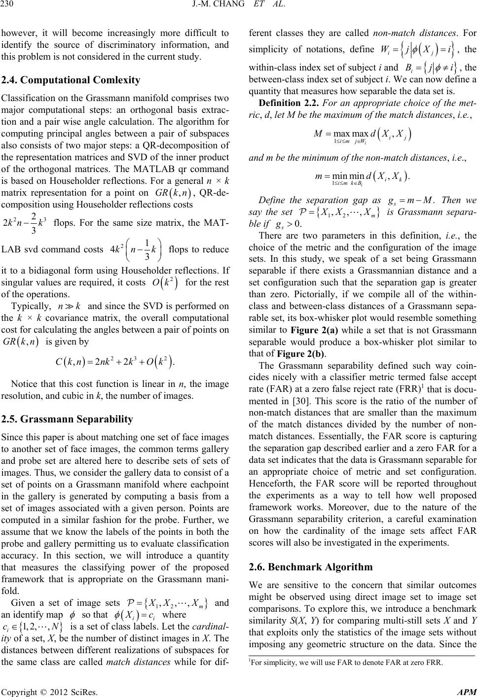

J.-M. CHANG ET AL.

230

however, it will become increasingly more difficult to

identify the source of discriminatory information, and

this problem is not considered in the current study.

2.4. Computational Comlexity

Classification on the Grassmann manifold comprises two

major computational steps: an orthogonal basis extrac-

tion and a pair wise angle calculation. The algorithm for

computing principal angles between a pair of subspaces

also consists of two major steps: a QR-decomposition of

the representation matrices and SVD of the inner product

of the orthogonal matrices. The MATLAB qr command

is based on Householder reflections. For a general n × k

matrix representation for a point on , QR-de-

composition using Householder reflections costs



,GRk n

kn k flops. For the same size matrix, the MAT-

LAB svd command costs 21

kn k

















23 2

2 .k Ok



,,,

flops to reduce

it to a bidiagonal form using Householder reflections. If

singular values are required, it costs for the rest

of the operations.

Typically, and since the SVD is performed on

the k × k covariance matrix, the overall computational

cost for calculating the angles between a pair of points on

is given by



,GR k



,2Ckn nk

Notice that this cost function is linear in n, the image

resolution, and cubic in k, the number of images.

2.5. Grassmann Separability

Since this paper is about matching one set of face images

to another set of face images, the common terms gallery

and probe set are altered here to describe sets of sets of

images. Thus, we consider the gallery data to consist of a

set of points on a Grassmann manifold where eachpoint

in the gallery is generated by computing a basis from a

set of images associated with a given person. Points are

computed in a similar fashion for the probe. Further, we

assume that we know the labels of the points in both the

probe and gallery permitting us to evaluate classification

accuracy. In this section, we will introduce a quantity

that measures the classifying power of the proposed

framework that is appropriate on the Grassmann mani-

fold.

Given a set of image sets 12

XX and

an identify map



so that











N where



1, 2,,c



i is a set of class labels. Let the cardinal-

ity of a set, X, be the number of distinct images in X. The

distances between different realizations of subspaces for

the same class are called match distances while for dif-

ferent classes they are called non-match distances. For









simplicity of notations, define Wj , the

within-class index set of subject i and



Bji







max max,

iij

im jW

i, the

between-class index set of subject i. We can now define a

quantity that measures how separable the data set is.

Definition 2.2. For an appropriate choice of the met-

ric, d, let M be the maximum of the match distances, i.e.,

dXX







min min,.

iik

imkB

mdXX





and m be the mi nimu m of the no n -match distances, i.e.,

Define the separation gap as .

mM Then we

say the set





,,,

XX

0.g is Grassmann separa-

ble if

There are two parameters in this definition, i.e., the

choice of the metric and the configuration of the image

sets. In this study, we speak of a set being Grassmann

separable if there exists a Grassmannian distance and a

set configuration such that the separation gap is greater

than zero. Pictorially, if we compile all of the within-

class and between-class distances of a Grassmann sepa-

rable set, its box-whisker plot would resemble something

similar to Figure 2(a) while a set that is not Grassmann

separable would produce a box-whisker plot similar to

that of Figure 2(b).

The Grassmann separability defined such way coin-

cides nicely with a classifier metric termed false accept

rate (FAR) at a zero false reject rate (FRR)1 that is docu-

mented in [30]. This score is the ratio of the number of

non-match distances that are smaller than the maximum

of the match distances divided by the number of non-

match distances. Essentially, the FAR score is capturing

the separation gap described earlier and a zero FAR for a

data set indicates that the data is Grassmann separable for

an appropriate choice of metric and set configuration.

Henceforth, the FAR score will be reported throughout

the experiments as a way to tell how well proposed

framework works. Moreover, due to the nature of the

Grassmann separability criterion, a careful examination

on how the cardinality of the image sets affect FAR

scores will also be investigated in the experiments.

2.6. Benchmark Algorithm

We are sensitive to the concern that similar outcomes

might be observed using direct image set to image set

comparisons. To explore this, we introduce a benchmark

similarity S(X, Y) for comparing multi-still sets X and Y

that exploits only the statistics of the image sets without

imposing any geometric structure on the data. Since the

1For simplicity, we will use FAR to denote FAR at zero FRR.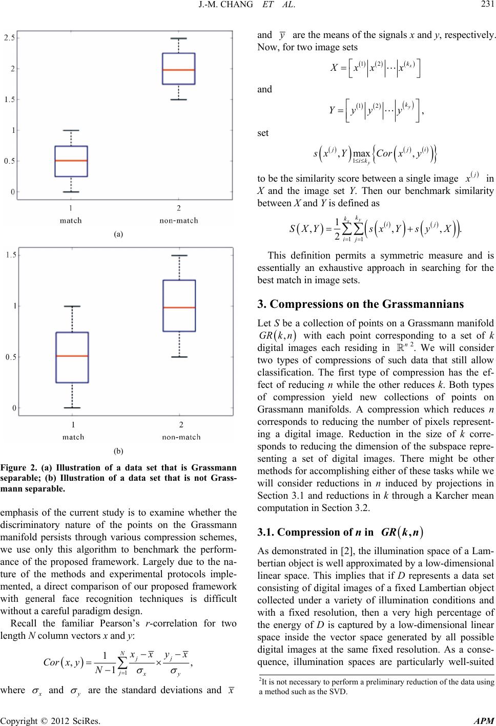

J.-M. CHANG ET AL. 231

(a)

(b)

Figure 2. (a) Illustration of a data set that is Grassmann

separable; (b) Illustration of a data set that is not Grass-

mann separable.

emphasis of the current study is to examine whether the

discriminatory nature of the points on the Grassmann

manifold persists through various compression schemes,

we use only this algorithm to benchmark the perform-

ance of the proposed framework. Largely due to the na-

ture of the methods and experimental protocols imple-

mented, a direct comparison of our proposed framework

with general face recognition techniques is difficult

without a careful paradigm design.

Recall the familiar Pearson’s r-correlation for two

length N column vectors x and y:



xy x





Corx yN



where



and



are the standard deviations and

and

are the means of the signals x and y, respectively.

Now, for two image sets

 



12 x

Xxx x













and



12 y

Yyy y



,













set





 







,max ,

jji

sx YCorxy





to be the similarity score between a single image

X and the image set Y. Then our benchmark similarity

between X and Y is defined as



,,,.

kij

SXYsx YsyX







This definition permits a symmetric measure and is

essentially an exhaustive approach in searching for the

best match in image sets.

3. Compressions on the Grassmannians

Let S be a collection of points on a Grassmann manifold





,GRk nn





,GRkn

with each point corresponding to a set of k

digital images each residing in 2. We will consider

two types of compressions of such data that still allow

classification. The first type of compression has the ef-

fect of reducing n while the other reduces k. Both types

of compression yield new collections of points on

Grassmann manifolds. A compression which reduces n

corresponds to reducing the number of pixels represent-

ing a digital image. Reduction in the size of k corre-

sponds to reducing the dimension of the subspace repre-

senting a set of digital images. There might be other

methods for accomplishing either of these tasks while we

will consider reductions in n induced by projections in

Section 3.1 and reductions in k through a Karcher mean

computation in Section 3.2.

3.1. Compression of n in

As demonstrated in [2], the illumination space of a Lam-

bertian object is well approximated by a low-dimensional

linear space. This implies that if D represents a data set

consisting of digital images of a fixed Lambertian object

collected under a variety of illumination conditions and

with a fixed resolution, then a very high percentage of

the energy of D is captured by a low-dimensional linear

space inside the vector space generated by all possible

digital images at the same fixed resolution. As a conse-

quence, illumination spaces are particularly well-suited

2It is not necessary to perform a preliminary reduction of the data using

a method such as the SVD.

J.-M. CHANG ET AL.

232

for classification on Grassmannians.

The approximated illumination space, as captured by a

k-dimensional approximation of the data set D, can be

represented by a point . Given a point

, let q denote the associated k-di-

mensional subspace. In typical settings, where n, m are

much larger than k, one expects a general linear map

to approximately preserve the inter-rela-

tionships among the principal angles between most sub-

spaces of . For instance, suppose Vp, Vq, Vr are three

k-dimensional subspaces of (corresponding to three

points ), suppose further that the

minimal principal angle between Vp and Vq is small

compared to the minimal principal angle between Vp and

Vr. Then under the general linear map L, one expects the

minimal principal angle between



,pGRkn

qGn







,Rk





nV





,, ,r GRkn





LV and





q to

be small compared to the minimal principal angle be-

tween



LV and .



There are several families of linear transformations

which are natural and useful to consider in the context of

face recognition. In this paper we will restrict our atten-

tion to a special family of linear transformations known

as patch projections, these should be considered as com-

plementary to patch collapsing. These terms are de-

scribed below:

1) (Patch Collapsing) Consider a partition of the com-

ponents of a vector, V, into disjoint sets 12d.

Patch collapsing is the operation of replacing, for each i

between 1 and d, the components in Pi with a fixed

weighted average of these components. This operation

can be expressed as a linear map, ,

. If L is further required to conserve energy then

and thus is a projection map. An example of

this type of projection is the partitioning of a digital im-

age into regions as provided by the scaling spaces in the

Haar wavelet decomposition. See Figure 3(a) for an il-

lustration of this type.

PP P

ndn



dn

LL L

PP P

2) (Patch Projection) Given a partition of the compo-

nents of a vector, V, into disjoint sets 12 d.

A family of patch projections is given by the natural pro-

jection maps ||

L,

PPn

:nm

L

. An example of a

patch projection is the restriction of a digital image to a

region of the image. For instance, the restriction of a

digital image of a face to the region surrounding the lips.

See Figure 3(b) for illustrations of several patch projec-

tions.

Patch projection is the focus of this paper, where a

patch of an image is simply a sub-image with resolution

much less than the original full image. Patch projections

are linear maps and illumination spaces are well ap-

proximated by linear spaces thus it is natural to study

patch illumination spaces through the mathematics asso-

ciated to parameter spaces of linear spaces. A few com-

ments on the relationship between projections and Grass-

mannians are in order.

Let K be the kernel of a linear map . Let









Ω,

GRk n denote the Schubert variety defined

 







Ω,dim 1.

KpGRknVK





L induces a natural map



 

:,Ω,

LGRknKGRkm

V

since the image of any k-dimensional subspace

under L remains k-dimensional precisely if the point





,pGRkn corresponding to V lies outside of





Ω

Suppose dim



, then



Ω

is a proper subset





,GRk n and the dimension of



Ω

is strictly

less than the dimension of . Thus, with prob-

ability one, a point chosen at random from



,GRk n





,GRk n

will lie in









,ΩGRk nK



,GRk n

. Due to the method we use

to determine points on , the quantization of

pixel values in digital images and the special nature of

patch projections, we are not choosing random points.

Thus it is possible for the corresponding linear spaces to

have a non-trivial intersection with the kernel of the pro-

jection map. However, as one might expect, we have yet

to observe a point accidently chosen to lie within





. Ω

The computational saving that is accomplished by this

type of compression is on the order of . For exam-

ple, using image patches of 30 × 30 instead of the origi-

nal 200 × 200 will enable a speedup that is roughly 44

times faster for a single pair wise distance calculation.



,GRkn3.2. Compression of k in

The notion of mean is often used as an initial estimator

for studying variability in a distribution. We anticipate

the use of mean subspaces, in object recognition prob-

lems that are cast on a Grassmannian, will provide us a

(a)

(b)

Figure 3. (a) An example of patch collapsing provided by

the scaling spaces in the Haar wavelet decomposition; (b)

Illustration of patch projections. Patches do not have to be

selected from a connected nor a rectangular region.

J.-M. CHANG ET AL. 233

blueprint to embed discriminatory information through

spaces of reduced dimensions. In this section, a quick

overview for calculating the mean subspace on





will be given followed by a proposed algorithm for per-

forming a robust classification at reduced computational

cost. We emphasize that it is the machinery associated

with the Grassmann manifold that permits this construc-

tion.

,GRk n



,GRkn

Although the definition of the Karcher mean is well-

established and it is easy to implement an algorithm for

its effective computation (see, e.g., [31,32]), the calcula-

tion of a Karcher mean can be rather expensive. Even on

a relatively small collection of sets, the computation can

fail to finish in a satisfactorily short period of time.By

incorporating low resolution feature patches in construc-

tion of the subject illumination spaces, as suggested in

this paper, the algorithm for calculating the Karcher

mean becomes computationally tractable. We now

briefly review the essential notations and algorithms for

calculating the Karcher mean for collections of points on

the Grassmann manifold.

Given points 1m, the Karcher mean

is the point q* that minimizes the sum of the geodesic

distances between q* and the pi’s, i.e.,

,,pp



, ,

qdqp







,dpq



,pGRknn



argmin 2

Rkn m





where is the geodesic distance between p and q

on the Grassmannian. We adopt a SVD-based algorithm

for computing the Karcher mean on a Grassmann mani-

fold as given in [33], which will be reviewed next.

Recall a point corresponds to a k-di-

mensional subspace of and can be represented by a

n × k matrix with orthonormal columns. Two matrices

with orthonormal columns, M, N determine the same

point in





,GRkn if and only if M = NQ for some k



where Ok is the orthogonal group of k × k matrices. The

tangent space to is given by



,R kn



,Rk



pG n









p Np







nk n

g

p





,,{

TGRknwwpqwwpq



 

where . Notice that  is the orthogonal

compliment of p. The EXPp map that takes a point in the

tangent space TG to a point in



,Rk





,GRk n



,GRkn

ossinU

DΘ.

wUV



,pGRkn





TGRkn

ΘT

qUV



1Σ

TT T

ppqpq UV



Θarctan Σ,

given by



Exp :,

TGRkn

where



wTGRknpV

hasthe The Logp map that takes a

point in a neighborhood of to a point in

is given by



TGRkn



Log :,

qU GRkn

with , where  and



when it is well-defined. A descent method

that utilizes the Exp and Log maps for finding the

Karcher mean on the Grassmann manifold is given in

Algorithm 2. For convergence results, see [33]. Next, we

describe an novel algorithm that utilizes Karcher mean





,GRk n







to construct a compressed representation

for a given collection of images that captures the intrinsic

variability of the subject illumination space.

Given a set of N images for a fixed subject class and

prescribe a Karcher representation dimension k, repeat

the following two steps for a total of t times, where t is a

number greater than 1 and usually much less than .

The purpose of the repetition is to capture the set vari-

ability exhibited in data set.

1) Randomly split the available data into two disjoint

setsof equal size each containing 2





images and the

data into so that





T



and are two points on

GR n













, where n is the resolution of the images.

2) Compute the first k left principal vectors of the pair

of subspaces





T



Q



mmt

m and and store the re-

sulting vectors in an n × k matrix, lm.

The collection of t principal vectors,



, corre-

sponds to t points on





,GRk n. A k-dimensional,

















mmt

l

, compressed representation of the illumina-

tion feature patch space for the subject class is then given

by the Karcher mean of the set via Algorithm

2 and is denoted by



. A detailed description of the

algorithm is given in Algorithm 3 with a schematic il-

lustration given in Figure 4.

Although Algorithm 3 is expensive even with the

low-resolution patch images due to the number of singu-

lar value decomposition it requires, the actual computa-

tions are done off-line. Moreover, each subject’s k-di-

mensional Karcher representation, with k much less than

Algorithm 2. Karcher mean on



,GRk n [33,34].





Inputs: Points 12

,,, ,

ppGRkn



, (machine precision).

Outputs: Karcher mean, q, of





,,,m

pp

1) Set



2) Find



1Log

m



3) If A





Σ.

UV A

, return q; else, go to step 4.

4) Find the SVD:



Update , go

to step 2.

cosΣsinΣqqV U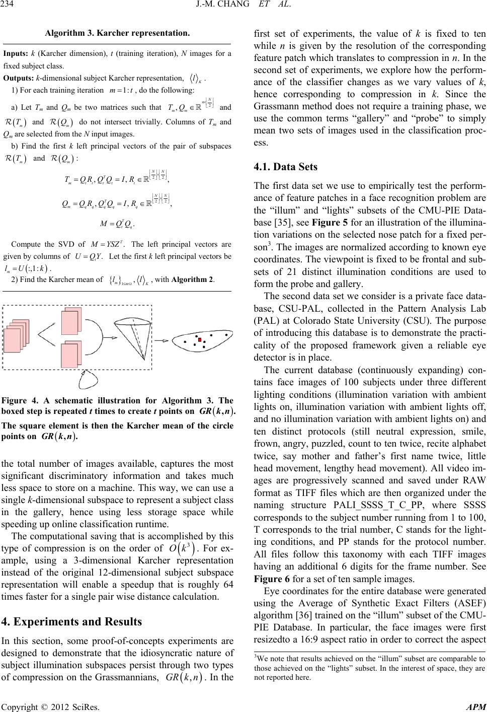

J.-M. CHANG ET AL.

234

Algorithm 3. Karcher representation.

Inputs: k (Karcher dimension), t (training iteration), N images for a

fixed subject class.

Outputs: k-dimensional subject Karcher representation, l

1:mt

1) For each training iteration , do the following:

a) Let Tm and Qm be two matrices such that 2





















Q

and



T and do not intersect trivially. Columns of Tman

Qm are selected from the N input images.

b) Find the first k left principal vectors of the pair of subspaces

and :



T





Q

,, ,

t t

IR 









TQRQQ

,, ,

q q

IR 









QQRQQ

QQ

Compute the SVD of .

YSZ

UQY



The left principal vectors are

given by columns of . Let the first k left principal vectors be



:,1: klU

2) Find the Karcher mean of



mmt

 , with Algorithm 2.

Figure 4. A schematic illustration for Algorithm 3. The

boxed step is repeated t times to create t points on





,GRk n



The square element is then the Karcher mean of the circle

points on



,GRk n



,GRk n

the total number of images available, captures the most

significant discriminatory information and takes much

less space to store on a machine. This way, we can use a

single k-dimensional subspace to represent a subject class

in the gallery, hence using less storage space while

speeding up online classification runtime.

The computational saving that is accomplished by this

type of compression is on the order of . For ex-

ample, using a 3-dimensional Karcher representation

instead of the original 12-dimensional subject subspace

representation will enable a speedup that is roughly 64

times faster for a single pair wise distance calculation.

4. Experiments and Results

In this section, some proof-of-concepts experiments are

designed to demonstrate that the idiosyncratic nature of

subject illumination subspaces persist through two types

of compression on the Grassmannians, . In the

first set of experiments, the value of k is fixed to ten

while n is given by the resolution of the corresponding

feature patch which translates to compression in n. In the

second set of experiments, we explore how the perform-

ance of the classifier changes as we vary values of k,

hence corresponding to compression in k. Since the

Grassmann method does not require a training phase, we

use the common terms “gallery” and “probe” to simply

mean two sets of images used in the classification proc-

ess.

4.1. Data Sets

The first data set we use to empirically test the perform-

ance of feature patches in a face recognition problem are

the “illum” and “lights” subsets of the CMU-PIE Data-

base [35], see Figure 5 for an illustration of the illumina-

tion variations on the selected nose patch for a fixed per-

son3. The images are normalized according to known eye

coordinates. The viewpoint is fixed to be frontal and sub-

sets of 21 distinct illumination conditions are used to

form the probe and gallery.

The second data set we consider is a private face data-

base, CSU-PAL, collected in the Pattern Analysis Lab

(PAL) at Colorado State University (CSU). The purpose

of introducing this database is to demonstrate the practi-

cality of the proposed framework given a reliable eye

detector is in place.

The current database (continuously expanding) con-

tains face images of 100 subjects under three different

lighting conditions (illumination variation with ambient

lights on, illumination variation with ambient lights off,

and no illumination variation with ambient lights on) and

ten distinct protocols (still neutral expression, smile,

frown, angry, puzzled, count to ten twice, recite alphabet

twice, say mother and father’s first name twice, little

head movement, lengthy head movement). All video im-

ages are progressively scanned and saved under RAW

format as TIFF files which are then organized under the

naming structure PALI_SSSS_T_C_PP, where SSSS

corresponds to the subject number running from 1 to 100,

T corresponds to the trial number, C stands for the light-

ing conditions, and PP stands for the protocol number.

All files follow this taxonomy with each TIFF images

having an additional 6 digits for the frame number. See

Figure 6 for a set of ten sample images.

Eye coordinates for the entire database were generated

using the Average of Synthetic Exact Filters (ASEF)

algorithm [36] trained on the “illum” subset of the CMU-

PIE Database. In particular, the face images were first

resizedto a 16:9 aspect ratio in order to correct the aspect

3We note that results achieved on the “illum” subset are comparable to

those achieved on the “lights” subset. In the interest of space, they are

not reported here.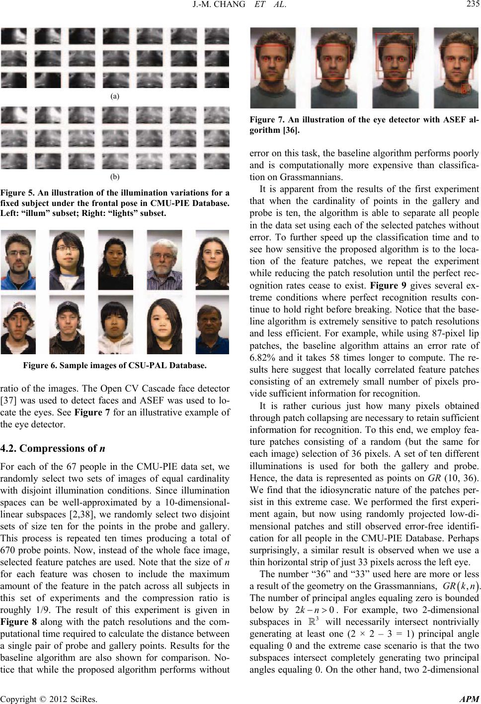

J.-M. CHANG ET AL. 235

(a)

(b)

Figure 5. An illustration of the illumination variations for a

fixed subject under the frontal pose in CMU-PIE Database .

Left: “illum” subset; Right: “lights” subset.

Figure 6. Sample images of CSU-PAL Database.

ratio of the images. The Open CV Cascade face detector

[37] was used to detect faces and ASEF was used to lo-

cate the eyes. See Figure 7 for an illustrative example of

the eye detector.

4.2. Compressions of n

For each of the 67 people in the CMU-PIE data set, we

randomly select two sets of images of equal cardinality

with disjoint illumination conditions. Since illumination

spaces can be well-approximated by a 10-dimensional-

linear subspaces [2,38], we randomly select two disjoint

sets of size ten for the points in the probe and gallery.

This process is repeated ten times producing a total of

670 probe points. Now, instead of the whole face image,

selected feature patches are used. Note that the size of n

for each feature was chosen to include the maximum

amount of the feature in the patch across all subjects in

this set of experiments and the compression ratio is

roughly 1/9. The result of this experiment is given in

Figure 8 along with the patch resolutions and the com-

putational time required to calculate the distance between

a single pair of probe and gallery points. Results for the

baseline algorithm are also shown for comparison. No-

tice that while the proposed algorithm performs without

Figure 7. An illustration of the eye detector with ASEF al-

gorithm [36].

error on this task, the baseline algorithm performs poorly

and is computationally more expensive than classifica-

tion on Grassmannians.

It is apparent from the results of the first experiment

that when the cardinality of points in the gallery and

probe is ten, the algorithm is able to separate all people

in the data set using each of the selected patches without

error. To further speed up the classification time and to

see how sensitive the proposed algorithm is to the loca-

tion of the feature patches, we repeat the experiment

while reducing the patch resolution until the perfect rec-

ognition rates cease to exist. Figure 9 gives several ex-

treme conditions where perfect recognition results con-

tinue to hold right before breaking. Notice that the base-

line algorithm is extremely sensitive to patch resolutions

and less efficient. For example, while using 87-pixel lip

patches, the baseline algorithm attains an error rate of

6.82% and it takes 58 times longer to compute. The re-

sults here suggest that locally correlated feature patches

consisting of an extremely small number of pixels pro-

vide sufficient information for recognition.

It is rather curious just how many pixels obtained

through patch collapsing are necessary to retain sufficient

information for recognition. To this end, we employ fea-

ture patches consisting of a random (but the same for

each image) selection of 36 pixels. A set of ten different

illuminations is used for both the gallery and probe.

Hence, the data is represented as points on GR (10, 36).

We find that the idiosyncratic nature of the patches per-

sist in this extreme case. We performed the first experi-

ment again, but now using randomly projected low-di-

mensional patches and still observed error-free identifi-

cation for all people in the CMU-PIE Database. Perhaps

surprisingly, a similar result is observed when we use a

thin horizontal strip of just 33 pixels across the left eye.

The number “36” and “33” used here are more or less

a result of the geometry on the Grassmannians,





The number of principal angles equaling zero is bounded

below by

,GRk n

20kn







. For example, two 2-dimensional

subspaces in will necessarily intersect nontrivially

generating at least one (2 × 2 – 3 = 1) principal angle

equaling 0 and the extreme case scenario is that the two

subspaces intersect completely generating two principal

angles equaling 0. On the other hand, two 2-dimensional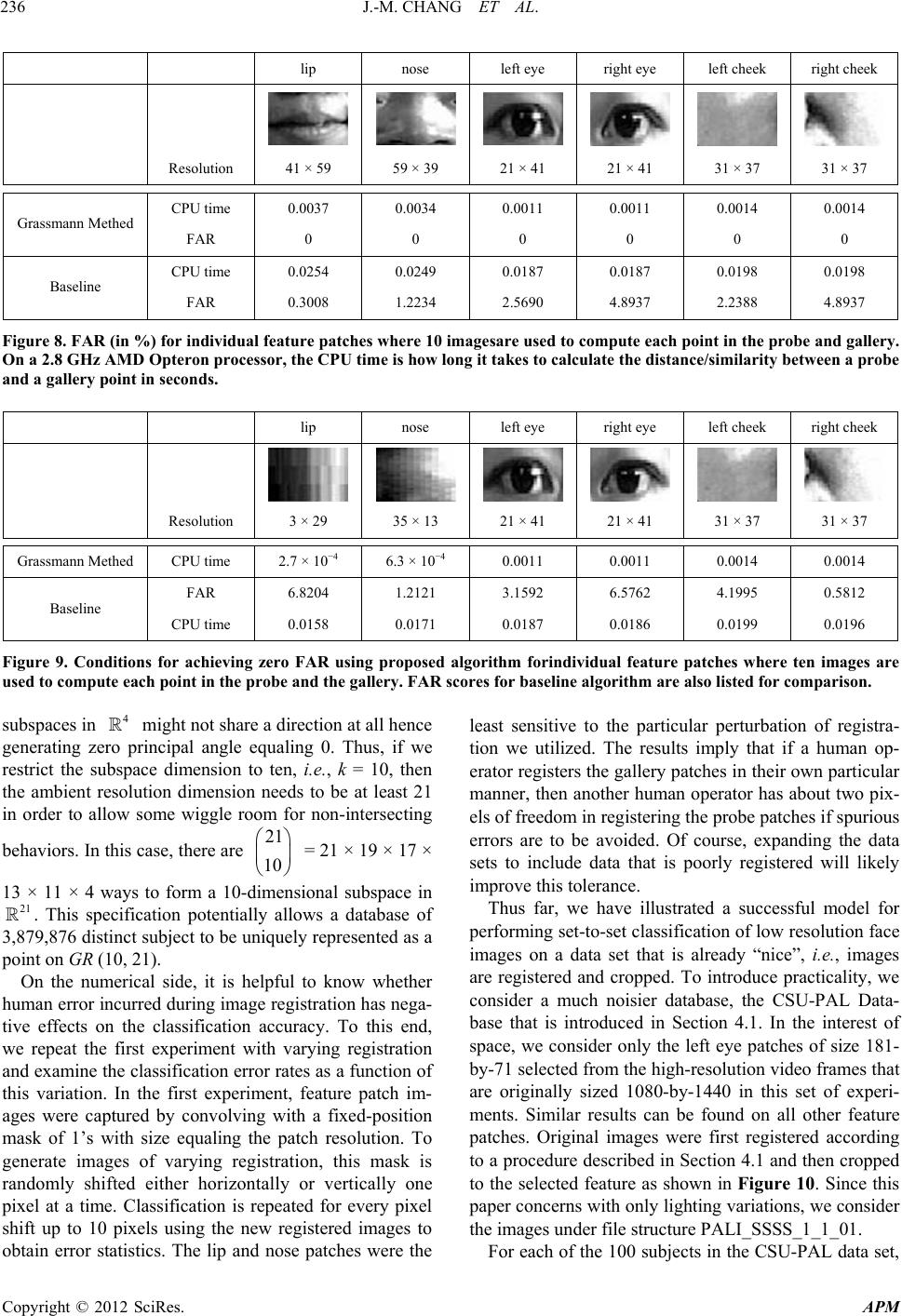

J.-M. CHANG ET AL.

236

lip nose left eye right eye left cheek right cheek

Resolution 41 × 59 59 × 39 21 × 41 21 × 41 31 × 37 31 × 37

CPU time 0.0037 0.0034 0.0011 0.0011 0.0014 0.0014

Grassmann Methed

FAR 0 0 0 0 0 0

CPU time 0.0254 0.0249 0.0187 0.0187 0.0198 0.0198

Baseline

FAR 0.3008 1.2234 2.5690 4.8937 2.2388 4.8937

Figure 8. FAR (in %) for individual feature patches w here 10 imagesare used to compute each point in the probe and gallery.

On a 2.8 GHz AMD Opteron processor, the CPU time is how long it takes to calculate the distance/similarity between a probe

and a gallery point in seconds.

lip nose left eye right eye left cheek right cheek

Resolution 3 × 29 35 × 13 21 × 41 21 × 41 31 × 37 31 × 37

Grassmann Methed CPU time 2.7 × 10−4 6.3 × 10−4 0.0011 0.0011 0.0014 0.0014

FAR 6.8204 1.2121 3.1592 6.5762 4.1995 0.5812

Baseline

CPU time 0.0158 0.0171 0.0187 0.0186 0.0199 0.0196

Figure 9. Conditions for achieving zero FAR using proposed algorithm forindividual feature patches where ten images are

used to compute each point in the probe and the gallery. FAR scores for baseline algorithm are also listed for comparison.

subspaces in might not share a direction at all hence

generating zero principal angle equaling 0. Thus, if we

restrict the subspace dimension to ten, i.e., k = 10, then

the ambient resolution dimension needs to be at least 21

in order to allow some wiggle room for non-intersecting











least sensitive to the particular perturbation of registra-

tion we utilized. The results imply that if a human op-

erator registers the gallery patches in their own particular

manner, then another human operator has about two pix-

els of freedom in registering the probe patches if spurious

errors are to be avoided. Of course, expanding the data

sets to include data that is poorly registered will likely

improve this tolerance.

behaviors. In this case, there are = 21 × 19 × 17 ×

13 × 11 × 4 ways to form a 10-dimensional subspace in

. This specification potentially allows a database of

3,879,876 distinct subject to be uniquely represented as a

point on GR (10, 21).

Thus far, we have illustrated a successful model for

performing set-to-set classification of low resolution face

images on a data set that is already “nice”, i.e., images

are registered and cropped. To introduce practicality, we

consider a much noisier database, the CSU-PAL Data-

base that is introduced in Section 4.1. In the interest of

space, we consider only the left eye patches of size 181-

by-71 selected from the high-resolution video frames that

are originally sized 1080-by-1440 in this set of experi-

ments. Similar results can be found on all other feature

patches. Original images were first registered according

to a procedure described in Section 4.1 and then cropped

to the selected feature as shown in Figure 10. Since this

paper concerns with only lighting variations, we consider

the images under file structure PALI_SSSS_1_1_01.

On the numerical side, it is helpful to know whether

human error incurred during image registration has nega-

tive effects on the classification accuracy. To this end,

we repeat the first experiment with varying registration

and examine the classification error rates as a function of

this variation. In the first experiment, feature patch im-

ages were captured by convolving with a fixed-position

mask of 1’s with size equaling the patch resolution. To

generate images of varying registration, this mask is

randomly shifted either horizontally or vertically one

pixel at a time. Classification is repeated for every pixel

shift up to 10 pixels using the new registered images to

obtain error statistics. The lip and nose patches were the For each of the 100 subjects in the CSU-PAL data set,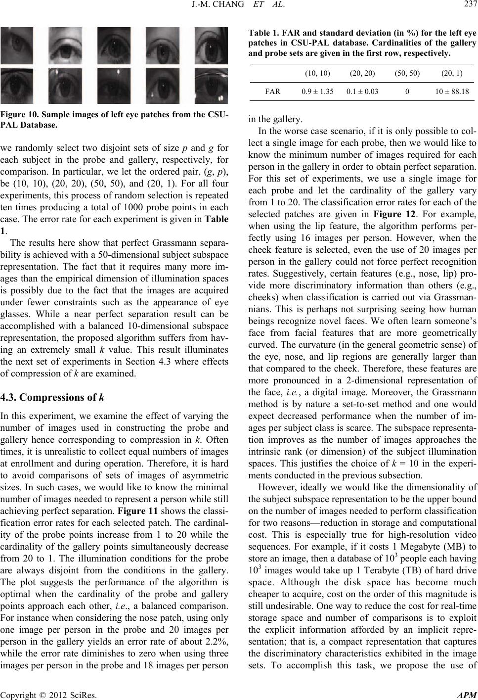

J.-M. CHANG ET AL. 237

Figure 10. Sample images of left eye patches from the CSU-

PAL Database.

we randomly select two disjoint sets of size p and g for

each subject in the probe and gallery, respectively, for

comparison. In particular, we let the ordered pair, (g, p),

be (10, 10), (20, 20), (50, 50), and (20, 1). For all four

experiments, this process of random selection is repeated

ten times producing a total of 1000 probe points in each

case. The error rate for each experiment is given in Table

The results here show that perfect Grassmann separa-

bility is achieved with a 50-dimensional subject subspace

representation. The fact that it requires many more im-

ages than the empirical dimension of illumination spaces

is possibly due to the fact that the images are acquired

under fewer constraints such as the appearance of eye

glasses. While a near perfect separation result can be

accomplished with a balanced 10-dimensional subspace

representation, the proposed algorithm suffers from hav-

ing an extremely small k value. This result illuminates

the next set of experiments in Section 4.3 where effects

of compression of k are examined.

4.3. Compressions of k

In this experiment, we examine the effect of varying the

number of images used in constructing the probe and

gallery hence corresponding to compression in k. Often

times, it is unrealistic to collect equal numbers of images

at enrollment and during operation. Therefore, it is hard

to avoid comparisons of sets of images of asymmetric

sizes. In such cases, we would like to know the minimal

number of images needed to represent a person while still

achieving perfect separation. Figure 11 shows the classi-

fication error rates for each selected patch. The cardinal-

ity of the probe points increase from 1 to 20 while the

cardinality of the gallery points simultaneously decrease

from 20 to 1. The illumination conditions for the probe

are always disjoint from the conditions in the gallery.

The plot suggests the performance of the algorithm is

optimal when the cardinality of the probe and gallery

points approach each other, i.e., a balanced comparison.

For instance when considering the nose patch, using only

one image per person in the probe and 20 images per

person in the gallery yields an error rate of about 2.2%,

while the error rate diminishes to zero when using three

images per person in the probe and 18 images per person

Table 1. FAR and standard deviation (in %) for the left eye

patches in CSU-PAL database. Cardinalities of the gallery

and probe sets are given in the first row, respectively.

(10, 10) (20, 20) (50, 50) (20, 1)

FAR 0.9 ± 1.350.1 ± 0.03 0 10 ± 88.18

in the gallery.

In the worse case scenario, if it is only possible to col-

lect a single image for each probe, then we would like to

know the minimum number of images required for each

person in the gallery in order to obtain perfect separation.

For this set of experiments, we use a single image for

each probe and let the cardinality of the gallery vary

from 1 to 20. The classification error rates for each of the

selected patches are given in Figure 12. For example,

when using the lip feature, the algorithm performs per-

fectly using 16 images per person. However, when the

cheek feature is selected, even the use of 20 images per

person in the gallery could not force perfect recognition

rates. Suggestively, certain features (e.g., nose, lip) pro-

vide more discriminatory information than others (e.g.,

cheeks) when classification is carried out via Grassman-

nians. This is perhaps not surprising seeing how human

beings recognize novel faces. We often learn someone’s

face from facial features that are more geometrically

curved. The curvature (in the general geometric sense) of

the eye, nose, and lip regions are generally larger than

that compared to the cheek. Therefore, these features are

more pronounced in a 2-dimensional representation of

the face, i.e., a digital image. Moreover, the Grassmann

method is by nature a set-to-set method and one would

expect decreased performance when the number of im-

ages per subject class is scarce. The subspace representa-

tion improves as the number of images approaches the

intrinsic rank (or dimension) of the subject illumination

spaces. This justifies the choice of k = 10 in the experi-

ments conducted in the previous subsection.

However, ideally we would like the dimensionality of

the subject subspace representation to be the upper bound

on the number of images needed to perform classification

for two reasons—reduction in storage and computational

cost. This is especially true for high-resolution video

sequences. For example, if it costs 1 Megabyte (MB) to

store an image, then a database of 103 people each having

103 images would take up 1 Terabyte (TB) of hard drive

space. Although the disk space has become much

cheaper to acquire, cost on the order of this magnitude is

still undesirable. One way to reduce the cost for real-time

storage space and number of comparisons is to exploit

the explicit information afforded by an implicit repre-

sentation; that is, a compact representation that captures

the discriminatory characteristics exhibited in the image

sets. To accomplish this task, we propose the use of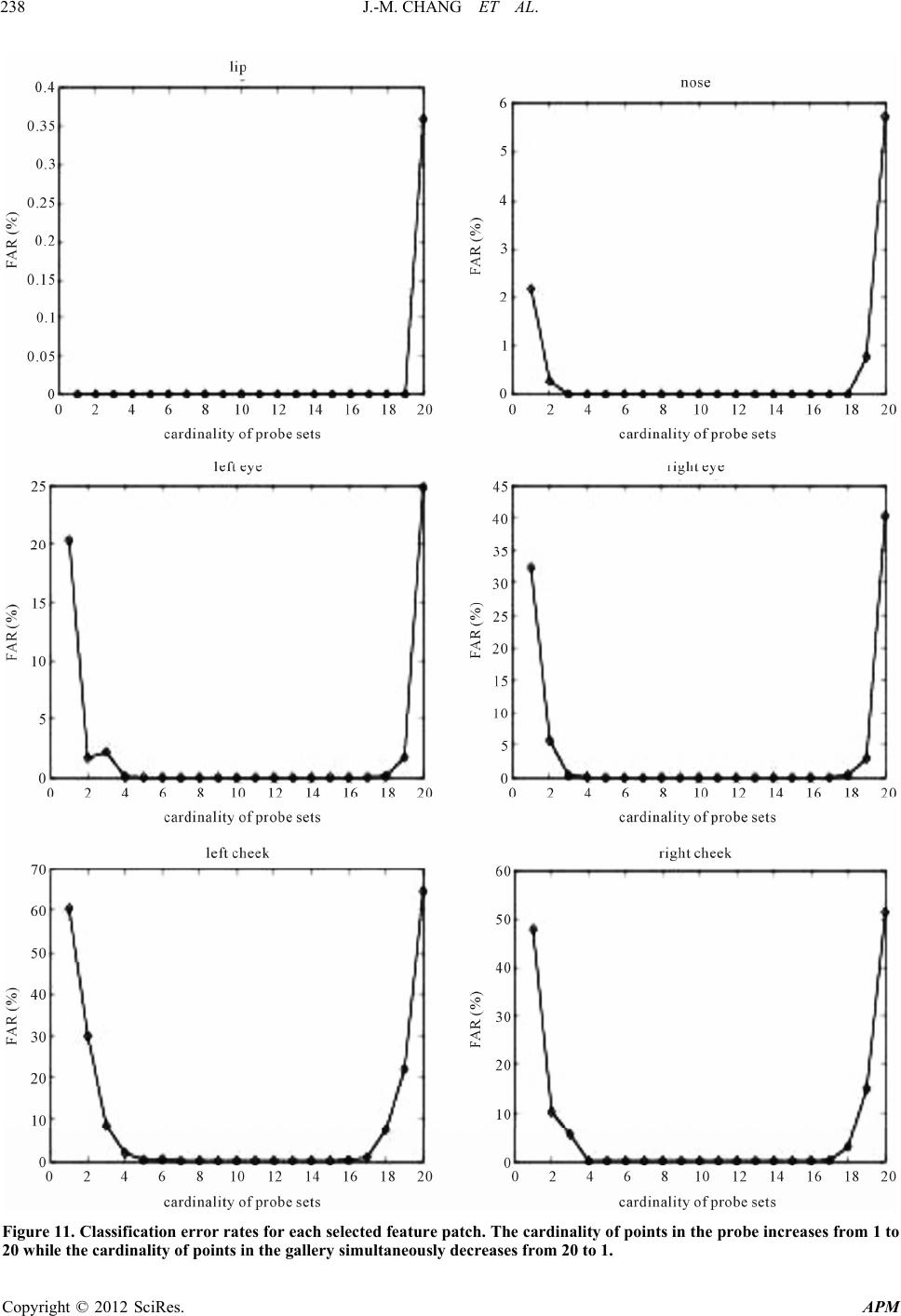

J.-M. CHANG ET AL.

238

Figure 11. Classification error rates for each selected feature patch. The cardinality of points in the probe increases from 1 to

20 while the cardinality of points in the gallery simultaneously decreases from 20 to 1.

J.-M. CHANG ET AL. 239

Figure 12. Classification error rates for each selected feature patch. The cardinality of the probe points is one while the car-

inality of the gallery points ranges from 1 to 20. d

J.-M. CHANG ET AL.

240



,GRN n



,GRk n

1kN



1iP

Karcher representation, as described in Algorithm 3, for

image sets on the Grassmannians and illustrate its poten-

tial use for data compression with the following experi-

ment on the CUM-PIE “lights” data set.

The way we validate whether this reduced representa-

tion can be used to replace the original image sets in the

face recognition tasks is to compare the respective classi-

fication error rates. If an error-free classification result

can be achieved on the original , then for a

Karcher representation to successfully compress the

same discriminatory information, the same error-free

result will need to be observed on for

. The optimal result will be an error-free classi-

fication when the compression is at its maximum, i.e.,

when k = 1. We will now describe the specific parame-

ters implemented in this validating experiment.

Let be an n × N matrix that stores all N gallery

images of each subject class for . Denote 1 ≤ k ≤







1iP



the dimensionality of the Karcher representation

which will be explored throughout the experiment. Fur-

ther let the cardinality of the probe sets be three for all

subjects and store the images in n × 3 matrices, ,

. For a fixed k, Algorithm 3 is used to obtain a

Karcher representation for each subject class,



where P is the total number of subjects in the gallery.

That is, each



,GRk n



resides in and can be

represented by a n × k matrix,

. If we cast the clas-

sification architecture in a distance matrix with the mini-

mal principal angle metric





,D

min j



 



dDKT

min

 

, then Karcher com-

pression provides useful compact representation if

P ij





ij 



P ij



, where , given that

with





59 4919

dD.

Let N = 16, the k-dimensional Karcher representation

resulted in an error-free classification for k ≥ 4 on the lip

patch of the “lights” data set (). In

comparison, using four raw images per subject in the

gallery resulted an average FAR of 30%. In the extreme

case, when only a single raw image is used, the classifier

returns an error rate of nearly 90%; while a 1-dimen-

sional Karcher representation returns a 1% error rate.

Figure 13 tabulates the error rate as a function of the

dimensionality of the Karcher representation as well as

the cardinality of the gallery image set.

41n

The fact that the compression of a raw point on





16,4159



4, 4159

GR to a Karcher representation on

, without diminishing performance, indi-

cates the promise of Karcher compression in the context

of classification of image sets via Grassmannians. On the

contrary, when using k raw images for each gallery point,

the error rate never reaches zero for any 1 ≤ k ≤ 8. The

fact that using a 4-dimensional Karcher representation

achieves a perfect recognition result while using four raw

images in the gallery does not indicates that Karcher

representations are able to pack useful discriminatory

information in a more efficient manner. This technique

can potentially be used to enable compact representations

computed from video sequences or data sets where a

large number of images is available for the gallery.

5. Summary and Discussions

In this paper, a geometric framework for the general

classification problem with image sets is reviewed. The

power of the method is due, in part, to the fact that the

geometry and statistics of the Grassmann manifold are

well-understood and provide useful tools for quantifying

the relationships between patterns. We made precise how

this geometric framework is translated in practical set-

tings. We show by ways of experiments that the pro-

posed Grassmann method is robust against resolution and

dimensionality reduction which corresponds to compres-

sion in both k and n in





,GRk n.

Although there might be other ways to accomplish ei-

ther of these two compressions, we consider compression

in n induced by mathematical projections and compres-

sion in k through the proposed Karcher representation.

Empirical results collected on a public database, CMU-

PIE, and a private database, CSU-PAL, verify claimed

success in employing a compressed representation

through the use of Karcher mean and mathematical pro-

jections on the Grassmannian in set-to-set classification.

These results are reported through an appropriate meas-

ure on the Grassmann manifold that coincides with a

classifier metric termed false accept rate at a zero false

reject rate, FAR for short.

The work presented here originated from our goal to

push the Grassmann method to a breaking point. While

Figure 13. Error rate comparisons with k-dimensional

Karcher representation and k raw images for points in the

gallery corresponding to lip patches. Three images are use d

to compute points in the probe.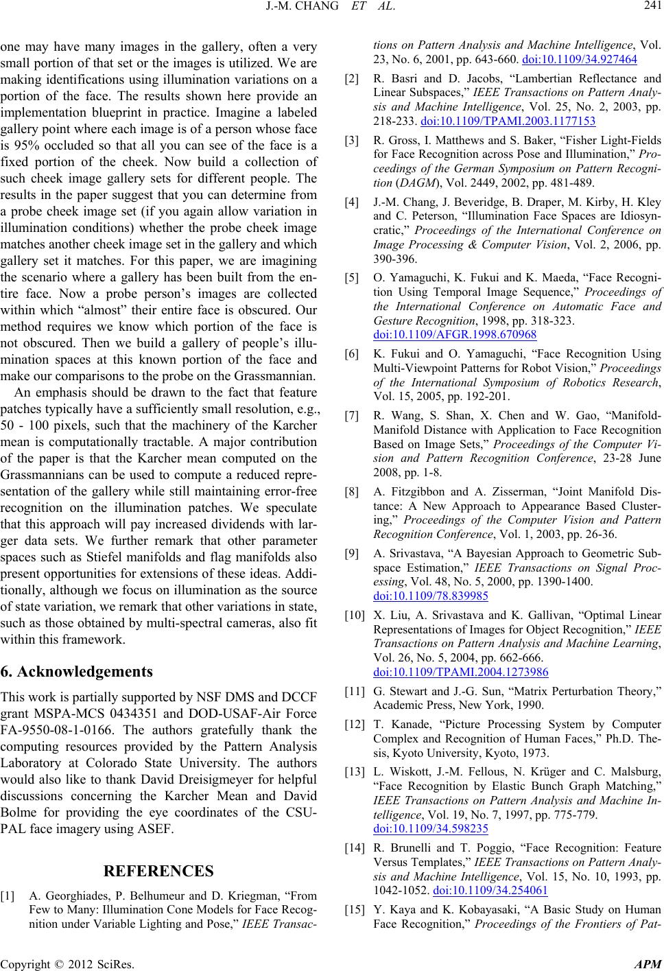

J.-M. CHANG ET AL. 241

one may have many images in the gallery, often a very

small portion of that set or the images is utilized. We are

making identifications using illumination variations on a

portion of the face. The results shown here provide an

implementation blueprint in practice. Imagine a labeled

gallery point where each image is of a person whose face

is 95% occluded so that all you can see of the face is a

fixed portion of the cheek. Now build a collection of

such cheek image gallery sets for different people. The

results in the paper suggest that you can determine from

a probe cheek image set (if you again allow variation in

illumination conditions) whether the probe cheek image

matches another cheek image set in the gallery and which

gallery set it matches. For this paper, we are imagining

the scenario where a gallery has been built from the en-

tire face. Now a probe person’s images are collected

within which “almost” their entire face is obscured. Our

method requires we know which portion of the face is

not obscured. Then we build a gallery of people’s illu-

mination spaces at this known portion of the face and

make our comparisons to the probe on the Grassmannian.

An emphasis should be drawn to the fact that feature

patches typically have a sufficiently small resolution, e.g.,

50 - 100 pixels, such that the machinery of the Karcher

mean is computationally tractable. A major contribution

of the paper is that the Karcher mean computed on the

Grassmannians can be used to compute a reduced repre-

sentation of the gallery while still maintaining error-free

recognition on the illumination patches. We speculate

that this approach will pay increased dividends with lar-

ger data sets. We further remark that other parameter

spaces such as Stiefel manifolds and flag manifolds also

present opportunities for extensions of these ideas. Addi-

tionally, although we focus on illumination as the source

of state variation, we remark that other variations in state,

such as those obtained by multi-spectral cameras, also fit

within this framework.

6. Acknowledgements

This work is partially supported by NSF DMS and DCCF

grant MSPA-MCS 0434351 and DOD-USAF-Air Force

FA-9550-08-1-0166. The authors gratefully thank the

computing resources provided by the Pattern Analysis

Laboratory at Colorado State University. The authors

would also like to thank David Dreisigmeyer for helpful

discussions concerning the Karcher Mean and David

Bolme for providing the eye coordinates of the CSU-

PAL face imagery using ASEF.

REFERENCES

[1] A. Georghiades, P. Belhumeur and D. Kriegman, “From

Few to Many: Illumination Cone Models for Face Recog-

nition under Variable Lighting and Pose,” IEEE Transac-

tions on Pattern Analysis and Machine Intelligence, Vol.

23, No. 6, 2001, pp. 643-660. doi:10.1109/34.927464

[2] R. Basri and D. Jacobs, “Lambertian Reflectance and

Linear Subspaces,” IEEE Transactions on Pattern Analy-

sis and Machine Intelligence, Vol. 25, No. 2, 2003, pp.

218-233. doi:10.1109/TPAMI.2003.1177153

[3] R. Gross, I. Matthews and S. Baker, “Fisher Light-Fields

for Face Recognition across Pose and Illumination,” Pro-

ceedings of the German Symposium on Pattern Recogni-

tion (DAGM), Vol. 2449, 2002, pp. 481-489.

[4] J.-M. Chang, J. Beveridge, B. Draper, M. Kirby, H. Kley

and C. Peterson, “Illumination Face Spaces are Idiosyn-

cratic,” Proceedings of the International Conference on

Image Processing & Computer Vision, Vol. 2, 2006, pp.

390-396.

[5] O. Yamaguchi, K. Fukui and K. Maeda, “Face Recogni-

tion Using Temporal Image Sequence,” Proceedings of

the International Conference on Automatic Face and

Gesture Recognition, 1998, pp. 318-323.

doi:10.1109/AFGR.1998.670968

[6] K. Fukui and O. Yamaguchi, “Face Recognition Using

Multi-Viewpoint Patterns for Robot Vision,” Proceedings

of the International Symposium of Robotics Research,

Vol. 15, 2005, pp. 192-201.

[7] R. Wang, S. Shan, X. Chen and W. Gao, “Manifold-

Manifold Distance with Application to Face Recognition

Based on Image Sets,” Proceedings of the Computer Vi-

sion and Pattern Recognition Conference, 23-28 June

2008, pp. 1-8.

[8] A. Fitzgibbon and A. Zisserman, “Joint Manifold Dis-

tance: A New Approach to Appearance Based Cluster-

ing,” Proceedings of the Computer Vision and Pattern

Recognition Conference, Vol. 1, 2003, pp. 26-36.

[9] A. Srivastava, “A Bayesian Approach to Geometric Sub-

space Estimation,” IEEE Transactions on Signal Proc-

essing, Vol. 48, No. 5, 2000, pp. 1390-1400.

doi:10.1109/78.839985

[10] X. Liu, A. Srivastava and K. Gallivan, “Optimal Linear

Representations of Images for Object Recognition,” IEEE

Transactions on Pattern Analysis and Machine Learning,

Vol. 26, No. 5, 2004, pp. 662-666.

doi:10.1109/TPAMI.2004.1273986

[11] G. Stewart and J.-G. Sun, “Matrix Perturbation Theory,”

Academic Press, New York, 1990.

[12] T. Kanade, “Picture Processing System by Computer

Complex and Recognition of Human Faces,” Ph.D. The-

sis, Kyoto University, Kyoto, 1973.

[13] L. Wiskott, J.-M. Fellous, N. Krüger and C. Malsburg,

“Face Recognition by Elastic Bunch Graph Matching,”

IEEE Transactions on Pattern Analysis and Machine In-

telligence, Vol. 19, No. 7, 1997, pp. 775-779.

doi:10.1109/34.598235

[14] R. Brunelli and T. Poggio, “Face Recognition: Feature

Versus Templates,” IEEE Transactions on Pattern Analy-

sis and Machine Intelligence, Vol. 15, No. 10, 1993, pp.

1042-1052. doi:10.1109/34.254061

[15] Y. Kaya and K. Kobayasaki, “A Basic Study on Human

Face Recognition,” Proceedings of the Frontiers of Pat-

J.-M. CHANG ET AL.

242

tern Recognition, 1972, pp. 265-290.

[16] J. Harris, “Algebraic Geometry: A First Course,” Springer,

Berlin, 1992.

[17] A. Edelman, T. Arias and S. Smith, “The Geometry of

Algorithms with Orthogonality Constraints,” SIAM Jour-

nal on Matrix Analysis and Applications, Vol. 20, No. 2,

1999, pp. 303-353. doi:10.1137/S0895479895290954

[18] A. Björck and G. Golub, “Numerical Methods for Com-

puting Angles between Linear Subspaces,” Mathematics

of Computation, Vol. 27, No. 123, 1973, pp. 579-594.

[19] A. Knyazev and M. Argentati, “Principal Angles between

Subspaces in a Based Scalar Product: Algorithms and

Perturbation Estimates,” SIAM Journal of Scientific Com-

puting, Vol. 23, No. 6, 2002, pp. 2008-2040.

doi:10.1137/S1064827500377332

[20] J. Beveridge, B. Draper, J.-M. Chang, M. Kirby, H. Kley

and C. Peterson, “Principal Angles Separate Subject Illu-

mination Spaces in YDB and CMU-PIE,” IEEE Transac-

tions on Pattern Analysis and Machine Intelligence, Vol.

31, No. 2, 2009, pp. 351-356.

doi:10.1109/TPAMI.2008.200

[21] M. Nishiyama, O. Yamaguchi and K. Fukui, “Face Rec-

ognition with the Multiple Constrained Mutual Subspace

Method,” Proceedings of the International Conference on

Audio- and Video-Based Biometric Person Authentication,

2005, pp. 71-80.

[22] M. Nishiyama, M. Yuasa, T. Shibata, T. Wakasugi, T.

Kawahara and O. Yamaguchi, “Recognizing Faces of

Moving People by Hierarchical Image-Set Matching,”

Proceedings of the Computer Vision and Pattern Recog-

nition Conference, 2007, pp. 1-8.

[23] Q.-S. Sun, Z.-D. Liu, P.-A. Heng and D.-S. Xia, “A

Theorem on the Generalized Canonical Projective Vec-

tors,” Pattern Recognition, Vol. 38, No. 3, 2005, pp. 449-

452. doi:10.1016/j.patcog.2004.08.009

[24] Q.-S. Sun, P.-A. Heng, Z. Jin and D.-S. Xia, “Face Rec-

ognition Based on Generalized Canonical Correlation

Analysis,” Advances in Intelligent Computing, Vol. 3645,

2005, pp. 958-967.

[25] J.-M. Chang, M. Kirby and C. Peterson, “Set-to-Set Face

Recognition under Variations in Pose and Illumination,”

Proceedings of the Biometrics Symposium, Baltimore,

11-13 September 2007, pp. 1-6.

doi:10.1016/j.patrec.2009.06.002

[26] T. Wang and P. Shi, “Kernal Grassmannian Distances and

Discriminate Analysis for Face Recognition from Image

Sets,” Pattern Recognition Letters, Vol. 30, 2009, pp.

1161-1165. doi:10.1016/j.patrec.2009.06.002

[27] J. Hamm and D. Lee, “Grassmann Discriminate Analysis:

a Unifying View on Subspace-Based Learning,” Pro-

ceedings of the 25th International Conference on Ma-

chine Learning, Vol. 307, 2008, pp. 376-383.

[28] M. Harandi, C. Sanderson, S. Shirazi and B. Lovell,

“Graph Embedding Discriminant Analysis on Grassman-

nian Manifolds for Improved Image Set Matching,” Pro-

ceedings of the Compute Vision and Pattern Recognition

Conference, 20-25 June 2011, pp. 2705-2712.

[29] H. Cevikalp and B. Triggs, “Face Recognition Based on

Image Sets,” Proceedings of the Compute Vision and Pat-

tern Recognition Conference, 13-18 June 2010, pp. 2567-

2573.

[30] A. Mansfield and J. Wayman, “Best Practices in Testing

and Reporting of Biometric Devices: Version 2.01,” Tech.

Rep. NPL Report CMSC 14/02, Centre for Mathematics

and Scientific Computing, National Physical Laboratory,

UK, 2002.

[31] H. Karcher, “Riemannian Center of Mass and Mollifier

Smoothing,” Communications on Pure and Applied Ma-

thematics, Vol. 30, 1977, pp. 509-541.

doi:10.1002/cpa.3160300502

[32] W. Kendall, “Probability, Convexity and Harmonic Maps

with Small Image I: Uniqueness and Fine Existence,”

Proceedings of the London Mathematical Society, Vol. 61,

1990, pp. 371-406. doi:10.1112/plms/s3-61.2.371

[33] E. Begelfor and M. Werman, “Affine Invariance Revis-

ited,” Proceedings of the Computer Vision and Pattern

Recognition Conference, Vol. 2, 2006, pp. 2087-2094.

[34] J. Manton, “A Globally Convergent Numerical Algorithm

for Computing the Center of Mass on Compact Lie

groups,” Proceedings of the International Conference on

Control, Automation, Robotics and Vision, Vol. 3, 2004,

pp. 2211-2216.

[35] T. Sim, S. Baker and M. Bsat, “The CMU Pose, Illumina-

tion, and Expression Database,” IEEE Transactions on

Pattern Analysis and Machine Intelligence, Vol. 25, No.

12, 2003, pp. 1615-1618.

doi:10.1109/TPAMI.2003.1251154

[36] D. Bolme, B. Draper and J. Beveridge, “Average of Syn-

thetic Exact Filters,” Proceedings of the Computer Vision

and Pattern Recognition, 20-25 June 2009, pp. 2015-

2112.

[37] P. Viola and M. Jones, “Robust Real-Time Face Detec-

tion,” International Journal of Computer Vision, Vol. 57,

No. 2, 2004, pp. 137-154.

doi:10.1023/B:VISI.0000013087.49260.fb

[38] P. Belhumeur and D. Kriegman, “What Is the Set of Im-

ages of an Object under All Possible Lighting Condi-

tions,” International Journal of Computer Vision, Vol. 28,

No. 3, 1998, pp. 245-260. doi:10.1023/A:1008005721484
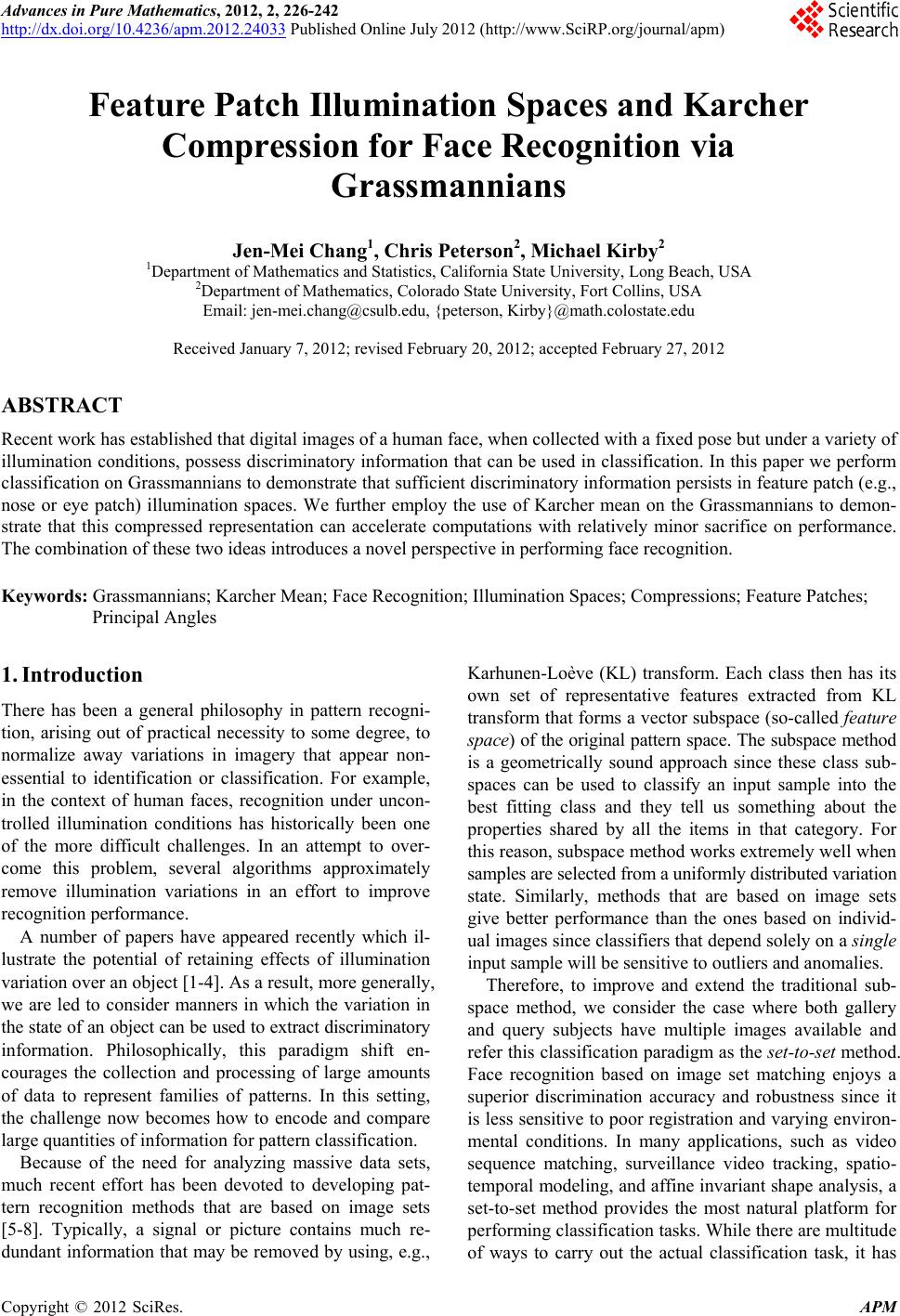