Received 23 March 2016; accepted 13 May 2016; published 17 May 2016

ABSTRACT

A mathematical model that makes use of data mining and soft computing techniques is proposed to estimate the software development effort. The proposed model works as follows: The parameters that have impact on the development effort are divided into groups based on the distribution of their values in the available dataset. The linguistic terms are identified for the divided groups using fuzzy functions, and the parameters are fuzzified. The fuzzified parameters then adopt associative classification for generating association rules. The association rules depict the parameters influencing the software development effort. As the number of parameters that influence the effort is more, a large number of rules get generated and can reduce the complexity, the generated rules are filtered with respect to the metrics, support and confidence, which measures the strength of the rule. Genetic algorithm is then employed for selecting set of rules with high quality to improve the accuracy of the model. The datasets such as Nasa93, Cocomo81, Desharnais, Maxwell, and Finnish-v2 are used for evaluating the proposed model, and various evaluation metrics such as Mean Magnitude of Relative Error, Mean Absolute Residuals, Shepperd and MacDonell’s Standardized Accuracy, Enhanced Standardized Accuracy and Effect Size are adopted to substantiate the effectiveness of the proposed methods. The results infer that the accuracy of the model is influenced by the metrics support, confidence, and the number of association rules considered for effort prediction.

Keywords:

Software Effort, Cost Estimation, Fuzzy Logic, Genetic Algorithm, Randomization Techniques

1. Introduction

Software development effort estimation is the process of predicting the most realistic use of effort required to develop or maintain the software based on incomplete, uncertain and/or noisy input. Software development effort is measured in terms of person hours or person months. Existing literature suggests that the expert estimation is the dominant strategy used for estimating the software development effort [1] . Construction of formal software effort estimation models has been the main focus in this area of research. Consequently many hybrid approaches have been developed to increase the efficiency of the methods. Improving the accuracy of the effort estimation models leads to effective control of time and budget during software development. We propose a hybrid model that combines fuzzy associative classification with genetic algorithm for estimating the development effort with high accuracy. The proposed model is evaluated using various evaluation metrics such as Mean Magnitude of Relative Error (MMRE), Mean Absolute Residuals (MAR), Shepperd and MacDonell’s metrics such as Standardized Accuracy (SA), enhanced SA and effect size. Experiments are carried out on the datasets Nasa93, Cocomo81, Desharnais, Maxwell, and Finnish-v2. The experimental results reveal that the proposed model yields satisfactory results in terms of accuracy.

2. Related Work

Expert estimation techniques have been widely consented in the software professionals; hence most of the research in the last decade has been focused on the expert estimation [2] - [5] . Jorgenson [1] evoked best practice guidelines and provided suggestions on how to implement them in software organizations. Jorgenson [6] [7] suggested the practical guidelines for expert judgment based software effort estimation, and Manifest on expert judgement and formal models. Hybrid approach for rule learning, induction, selection and extraction in fuzzy rule based systems was introduced, and the model combines fuzzy rule based system along with Genetic Algorithms (GA) and expert judgement automation using Pittsburgh approach [8] . It was suggested to eliminate unnecessary linguistic terms. To increase the performance and reduce complexity of the Fuzzy logic based methods such as fuzzy membership function [9] is used. The GA based feature selection and machine learning methods have been used for parameters optimization in software effort estimation [10] . Random prediction is employed for different dataset and Standardized accuracy was evaluated through random prediction [11] . Software defect association mining suggested that high support and confidence levels may not result in higher prediction accuracy and a sufficient number of rules is a precondition for high prediction accuracy [12] . Ensembles of learning machine are applied to improve software cost estimation [13] . Menzies [14] suggested four kinds mining such as algorithm mining, landscape mining, decision mining and discussion mining to predictive modelling. Estimation by analogy can be significantly improved by dynamic selection of nearest neighbors in project data [15] .

From the analysis of the literature, it is found that the performance of the neural network is influenced by the change in dataset. This raises following research questions: 1) Whether the use of different datasets affect the results of the hybrid model? 2) Whether the changes in the values of the parameters such as support and confidence will improve the performance of the hybrid system or not?

The main reason for combining fuzzy associative classification with genetic algorithm is to fuzzify the dataset because the input dataset is in the mixed form with continuous and discrete values. Large numbers of rules are generated for rule generation. In order to avoid processing of large number of rules and avoid the memory space problem, support and confidence metrics are used to filter the rules. Rule pruning algorithm provides the initial population of rules for Genetic algorithm based search. Genetic algorithm is applied on pre-generated rules for picking out the best ones. Finally defuzzification is applied to the best rules. The major contribution in this work is creation of a hybrid model for estimation of software development effort. On analysis on the results obtained for different datasets, it can be observed that i) minimum support and minimum confidence influence on the dataset having attribute count less than ten, and high support and high confidence influence on the dataset having attribute count greater than twenty five. ii) External population is used to store high quality rules generated in the intermediate generations. iii) Random guessing is achieved through multithreading.

The proposed approach, a novel hybrid methodology, focuses on the combination of soft computing techniques to estimate the software effort accurately. This method is based on fuzzy associative classification with genetic algorithm to estimate the software effort efficiently. This paper is organized as follows: Section III presents the proposed model, Section IV presents results and discussions, and the conclusions are presented in the last section.

3. Proposed Model

Software project managers are always interested to know the effort involved in carrying out software tasks. The degree of accuracy achieved using each model varies with evaluation criteria. To improve the accuracy and to avoid the dependency of effort and cost estimation on number of lines of code (LOC), we propose a hybrid computational intelligence approach that combines fuzzy, association rule mining and evolutionary computation concepts. The main objective of the work is to design a model for estimating the effort for a software development project. The effort estimated should be more accurate, which means the estimated effort should not deviate much from the actual effort. The proposed system combines the machine learning techniques like Fuzzy Set Theory, Association Rule Mining and Genetic Algorithms. The dataset available in the PROMISE repository is used for training and testing. First, the training dataset is used to design the effort estimation model. The model thus developed can be used for predicting the effort for software projects that needs to be developed. The model developed is evaluated using the test set data, and Mean Magnitude Relative Error (MMRE) is used as the evaluation metric. Apart from MMRE, various metrics considered are Mean Absolute Residuals (MAR), Shepperd and MacDonell’s metric Standardised Accuracy (SA) and Effect size [11] . The proposed system is implemented in Java using Netbeans IDE. The implementation is divided into four sections namely, fuzzification, associative rule generation, rule pruning and Defuzzification. Figure 1 shows the workflow of the proposed model.

The work towards the proposed model is sequenced as follows.

3.1. Data Pre-Processing

The dataset is preprocessed before mining the data, analyzed, and the number of attributes is identified. The linguistic terms are defined for each attribute available in the dataset. The number of linguistic terms defined for each attribute is decided based on the distribution of values among the records available in the dataset. The linguistic terms assumed are the fuzzy sets or membership functions (MFs) defined for the attribute. The boundary values for the MFs are also defined. Two thirds of entire dataset is used as training set for generating the model. Data pre-processing involves analysis on the dataset: (i) Identifying the fuzzy sets, i.e., generation of fuzzy partitions for the numerical attributes, (ii) defining the type of MF to be used for each attribute, and (iii) defining the boundaries for the MFs.

3.2. Fuzzification

The training dataset is fed into the fuzzifier to convert the continuous values to linguistic terms, and the degrees to which they belong to each of the appropriate fuzzy sets via MFs are identified. Trapezoidal MF is used for all attributes in the proposed system.

3.3. Rule Generation

The relationships among the variables are represented by means of rules. The rules are of the following form:

“Antecedent proposition” → “consequent proposition”. These rules are generated using the associative classifier. The antecedent proposition is always a fuzzy proposition of the type “X1 is Nominal” → “X2 is High” where X1 is a linguistic variable and Nominal is a linguistic constant (term), X2 is the consequent variable and High is a consequent class. For example, the rules framed using Desharnais dataset are as follows:

If Team experience (Teamexp) is Low and Manager experience (Mgrexp) is Low then Effort is Very Low.

If Teamexp is Medium and Mgrexp is Medium and Transactions is Very Low, then Effort is High.

If Teamexp is Medium and Length is Low then Effort is Very Low.

where Teamexp, Mgrexp, Transactions, Length, etc. are attributes and Effort is the consequent attribute. Low, Medium, Very Low are linguistic terms associated with each attribute respectively.

3.4. Rule Pruning

The number of rules thus generated will be so large, since the dataset holds large number of attributes as well as the membership functions for each attribute is also more. To avoid this, we extract rules which frequently occur in the dataset based on the rule quality metrics like support and confidence. Instance frequent single items A and B, if we intersect the row Ids sets of A and B, then the resulting set should represent the tuples where A and B happen to be together in the training data. Therefore the classes associated with can be easily located, in which the support and confidence can be accessed and calculated. Then they will be used to decide whether or not is a frequent item and a candidate rule in the classifier. Since the training data have been scanned once to discover and generate the rules, this approach is highly effective in runtime and storage because it does not rely on the traditional approach of discovering frequent items, which requires multiple scans. After having generated all patterns, rules can be generated out of them. The task is to generate all possible rules in the frequent itemsets. Combine itemset and consequent class to generate Association rules and store intersecting row ids.

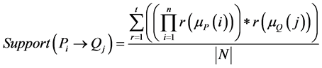
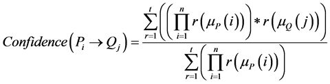
The total number of rules generated will be so large and hence some of them can be removed based on the rule quality metrics like Support and Confidence. Support gives how frequently the item occurs in the dataset. Confidence is a measure of the strength of the rule. The formulae for support and confidence metrics including fuzzy membership values are as follows.

(1)

(2)

where is the MF of antecedent while is the MF of consequent, and N is the total number of fuzzified

records, t is the total number of matched records in the dataset. The threshold values for support and confidence values are defined manually. Once a rule has passed the MinSupp threshold, the code then checks whether or not the rule passes the MinConf threshold. If the item confidence is larger than MinConf, then it will be generated as a candidate rule in the classifier. Otherwise, the item will be discarded. Thus, all items that survive MinConf are generated as candidate rules in the classifier. Thus the rules that have support and confidence greater than the threshold values are regarded as interesting. Frequent sets that do not include any interesting rules do not have to be considered anymore. All the discovered rules can in the end be presented to the user with their support and confidence values.

3.5. Rule Selection

The best co-operative rules are selected by means of Genetic Algorithm using Accuracy as the parameter. Thus, the output of this module provides best set of rules that helps in prediction. After filtering the rules based on support and confidence values, the best cooperative rules are selected by using evolutionary optimization techniques like Genetic Algorithms (GA). The rules extracted by GA focuses on improving the accuracy of the model being developed. The parameter settings of the genetic algorithm are as follows:

Initial population = Pruned Rules after support, confidence filtering; Number of generations = {5 - 500}; Cross over rate = 0.9; Mutation rate = 0.05.

The algorithm for extracting best set of rules for predicting the effort using GAs is explained as follows.

The solutions (rules) obtained in the rule generation module is used as input to GA. The rules so generated are binary encoded. For example, consider the rule generated for Desharnais dataset is of the form: Teamexp is Low and Mgrexp is Low→Effortis Low.

Each attribute Team experience, Manager experience has three linguistic variables Low, Medium and High defined for each, and Effort has five linguistic variable very low, low, medium, high, very high. Then the binary encoded rule is of the form 010,001,000,00000,000,000,00000,000,00001. Three digits are used for representing the attribute (except attribute transaction, adjustment and effort) and five digits are used for representing the attributes transaction, adjustment and effort. Binary encoding for attributes is done with bits of non-uniform length of 33 bits for Desharnais dataset.

In three bit representation, the presence of 1 in the least significant position represents that the attribute falls in the Low region and 1 at the most significant position represents the High region. Presence of 1 at the middle says that the value of the attribute lies in the middle region. In Five bit representation 00001 represents very low, 00010 represents low, 00100 represents medium, 01000 represents high, 10000 represents very high. The binary encoded solution is then used for evaluating the accuracy. Since the goal of the project is to maximize the accuracy, the accuracy itself is used as the objective function. The formula for computing the accuracy is as follows.

(3)

where, TP―true positive (i.e., number of positive cases correctly classified as belonging to the positive class); TN―true negative (i.e., number of negative cases correctly classified as belonging to the positive class); FP―false positive (i.e., number of negative cases misclassified as belonging to the positive class); FN―false negative (i.e., number of positive cases misclassified as belonging to the negative class).

After evaluating the fitness function for each rule, the rules greater than the threshold value defined for accuracy are stored in the external population. The external population is used to store the high quality set of rules in each generation. No genetic operators are applied in this external population. The final population of GA may leave out some of the high quality rules generated in the intermediate generations, and hence an external population is used. Reproduction or Selection is the first genetic operator applied on population. Chromosomes are selected from the population to be parents to cross over and produce offspring. Roulette Wheel selection is used as the selection strategy for selecting individuals. This method selects individual that can be used in the next generation of solutions with a probability proportional to the fitness. The more accurate rules have higher probabilities of being moved to the next generation. Cross over operator is applied to the mating pool with a hope that it would create better offspring. This operator proceeds in three steps. First, it selects at random a pair of individual strings for mating, then a cross-site is selected at random along the string length and the position values are swapped between two strings following the cross site. Multi-point crossover is employed for crossing the individuals. Since there are numerous attributes present in each rule, this technique is employed. Consider two rules which are chosen as parents for crossover operation. Attributes like team experience and length is the cross over sited. The first three bits and third three bits of parent1 are interchanged with the first and third three bits of parent 2. Figure 2 shows a Cross-over operation: before mating and after mating of Desharnais dataset. Mutation is carried out if the following two constraints are satisfied: (i) A rule is framed without antecedent but with consequent, and (ii) When an already existing individual is reproduced again by crossover or mutation operation. The solutions are then decoded. The process repeats with the rules framed after crossover and mutation

3.6. Defuzzification

The test set consisting of records for which effort needs to be predicted is fed into the defuzzifier. Using the best set of rules obtained from the rule selection module, the output (effort) is identified. The output so obtained is a linguistic term which is defuzzified to get a crisp value which gives the Effort in Person-hours or Person- months.

The rule selection module produces set of rules that are more accurate with regard to the training dataset. The defuzzifier is used for testing the model developed against the test set. The test set (one-third of records) especially not in the training set is fed as input to the defuzzifier. It makes use of the best set of rules produced by the rule selection module to predict the output. If n number of rules satisfies the test set record, then those n rules are considered for predicting the output. The formulae for defuzzification and effort calculation are as follows.

(4)

(5)

where is the MF of consequent, and is the centre value of expected interval of target stage in his-

torical dataset. The rule confidence is defined as TP/(TP+FN) in the high quality set of rules. The model was then evaluated using the Mean Magnitude of Relative Error (MMRE). The Magnitude of Relative Error (MRE) is defined as follows.

(6)

The MRE value was calculated for each observation i whose effort is predicted. The aggregation of MRE over multiple observations (N) can be achieved through the MMRE as follows.

(7)

The model was then evaluated using the Mean Absolute Residual (MAR), Standardised Accuracy and effect size. The Mean Absolute Residual (MAR) is defined as the mean value of the absolute difference between the actual and predicted effort. n is denoted as number of observations.

(8)

where n is denoted as number of observations. The SA measure [11] is defined as the ratio represents how much better P_i is than random guessing.

(9)

where is the mean value of a large number, typically 1000, runs of random guessing. This is defined as predict a for the target case t by randomly sampling (with equal probability) over all the remaining n-1 cases and where r is drawn randomly from. The effect size is defined as,

(10)

where is the sample standard deviation of the random guessing strategy.

4. Results and Discussion

4.1. NASA93 Dataset

The NASA dataset consists of 93 records and 27 attributes. One dependent variable is denoted as effort in the dataset.

Results focused on Accuracy and Effect size: For variation in the parameters Support and Confidence, the proposed model is evaluated using the following metrics: Accuracy, Error and Time taken for execution. Table 1 shows the results for Nasa93 datasets. From the analysis of Table 1, high support with high confidence gets constant SA value 43.94%. This higher SA value shows that the prediction system is better than the random guessing. No rules are formed above the support value 0.9. According to Software Defect Association mining and Defect correction effort prediction [12] , the results suggested that a sufficient number of rules influence on the accuracy rather than high support and confidence values. But this proposed model influence on both the constraints: high support and confidence as well as the number of rules. Effect size either measures the size of associations or the sizes of differences. From Table 1 it can be noted that “Small” effect size is obtained for the proposed model. According to the effect size mentioned in [11] , the “small” effect size obtained indicates that the model is statistically significant.

Instead of taking the mean of Absolute Residuals for all the 1000 runs, the worst value of ARs obtained (i.e., ARs of records with worst predicted values) during each iteration is taken and the mean is calculated. The mean

so calculated is substituted in Equation (9) instead of. The new enhanced evaluation metric standardized Accuracy is defined as

(11)

where is taken as the average of the worst values of absolute residuals obtained for each run of random

guessing. The values of SA obtained with the above formulae lie within the range of 89%-91%. The average training time required was 389 seconds. The average testing time for the proposed model is 773 seconds.

Results focused on running time of Random guessing: To improve the efficiency of the model, multithreading is employed for generating thousand runs of random guessing. If one-third of the data consisting of 30 records is used for random guessing, then the results need to be predicted for 30,000 records in thousand runs. In a seriali-

zation process, each iteration takes three seconds, thereby taking 3000 seconds for thousand iterations, while the time taken for model generation is less than 400 seconds. To obviate this problem, we have employed multi- threading since each iteration is independent of the previous iteration. Twenty iterations per thread are created, totally 50 threads are created. It requires six minutes for the multithreading process.

4.2. COCOMO81 Dataset

COCOMO81 data set consists of 63 records and 27 attributes. One dependent variable is denoted as effort in the dataset. All the variables except id are considered for predicting the effort.

Results focused on Accuracy and effect size: Table 2 shows that minimum number of rules is obtained for a support and confidence value of 0.9 and 0.3 respectively. The corresponding SA value obtained is 69.34%. It can be observed that support, confidence and sufficient number of rules influence on the accuracy of the estimated effort. The SA values obtained for different values of support and confidence are positive values which justify that the proposed prediction system is more dependable than the random guessing. It can also be noted that “Small” effect size is obtained which states that the model generated is statistically significant. However the values of standardized accuracy are in the higher range (i.e., 92% to 96%) for the average worst value of Absolute Residuals. This dataset gets higher SA value compared to all the other datasets. The average training time for COCOMO model was 154 seconds. Average testing time was 778 seconds for COCOMO model. The running time for random guessing is 4 seconds.

4.3. Desharnais Dataset

Desharnais data set consists of 81 records and 12 attributes. One dependent variable is denoted as effort in the dataset. In our proposed method the eight independent variables are taken from the description of the linear regression model of the dataset. The variables other than project ID, Year end and Points Non Adjust are considered for predicting the effort which is the output variable.

Results focused on Accuracy and effect size: From Table 3, SA value of 47.92% was observed for 0.03 support and 0.9 confidence values. Besides the value of SA metric is positive for all notices which indicate that the

proposed prediction system is better than random predictions. One of the MMRE values obtained is 105.45% for higher SA; hence this MMRE is as biased metric. According to the objective of the model, changing support and confidence values results in changes in SA. The small and medium effect size is also retained in this dataset which is statistically significant. However the values of SA are in the higher range (i.e., 76% to 86%) for the average worst value of Absolute Residuals. Running time (both training and testing) for Desharnais dataset is lesser than the Running time for other three datasets with 26 attributes. The average training time for Desharnais dataset is 136 seconds. The average testing time was 24 seconds. The running time of the random guessing is 6 seconds.

4.4. Maxwell Dataset

Maxwell data set consists of 62 records and 27 attributes. One dependent variable is denoted as effort in the dataset. The other independent variables are Start year of the project, Application type, Hardware platform, Database, User interface, Where developed, Telon use, Number of different development languages used, Customer participation, Development environment adequacy, Staff availability, Standards use, Methods use, Tools use, Software’s logical complexity, Requirements volatility, Quality requirements, Efficiency requirements, Installation requirements, Staff analysis skills, Staff application knowledge, Staff tool skills, Staff team skills, Duration, Size, Time and Effort. The attribute Start year of the project is not considered for predicting the effort.

Results focused on Accuracy and effect size: From Table 4, it is noted that positive values are sustained for SA which states that the prediction system is better than Random guessing. The maximum value of SA i.e., 40.84%, is obtained from this model. It is observed that high support, high confidence and sufficient number of rules influence on SA value. The “small” effect size is obtained for Maxwell dataset. However the values of SA are in higher range (i.e., 87.5% to 88.5%) for the average worst value of Absolute Residuals. The average training time was 1208 seconds and average testing time was 694 seconds. The running time for random guessing is 3 seconds

4.5. Finnish-v2 Dataset

Finnish-v2 data set consists of 38 records and 7 attributes. One dependent variable is denoted as development effort in the dataset. The variables other than project ID are considered for predicting the development effort.

Results focused on accuracy and effect size: Table 5 shows that SA has positive values; hence prediction

system is better than Random guessing. A maximum of 63.77% SA is achieved through high support, high confidence and with sufficient number of rules in this proposed model. The “large” effect size is obtained for Finnish-v2 dataset. However the values of SA are in the higher range (i.e., 78.33% to 85.02%) for the average worst value of Absolute Residuals. The average training and testing time for Finnish dataset is 31 seconds and 2 seconds. The running time of the random guessing for Maxwell dataset is 2 seconds.

5. Conclusion

The proposed model makes use of data mining and soft computing techniques for identifying the effort required for developing a software. The datasets in the PROMISE repository is used for evaluating the proposed model. The followings are the upsides of the proposed model: 1) Instead of scanning the dataset multiple times for generating rules and for calculation of support and confidence, the dataset is scanned only once to achieve both for improving the efficiency of the model; 2) Proposed Model produces improvement in accuracy for the considered datasets; 3) Random guessing for large number of runs is found out with the help of multithreading. Changes in the support and confidence value result in changes in the SA value for the proposed model. Enhanced SA metric is evaluated with different support and confidence value. Experimental results reveal that high support, high confidence and sufficient number of rules have an influence on the accuracy of the proposed model. This work can be extended to defect prediction.

Cite this paper

S. Saraswathi,N. Kannan, (2016) A Hybrid Associative Classification Model for Software Development Effort Estimation. Circuits and Systems,07,824-834. doi: 10.4236/cs.2016.76071

References

- 1. Jorgensen, M. (2004) A Review of Studies on Expert Estimation of Software Development Effort. Journal of Systems and Software, 70, 37-60.
http://dx.doi.org/10.1016/s0164-1212(02)00156-5 - 2. Araujo, R.A., Soares, S. and Oliveria, A.L.I. (2012) Hybrid Morphological Methodology for Software Development Cost Estimation. Expert Systems with Applications, 39, 6129-6139.
http://dx.doi.org/10.1016/j.eswa.2011.11.077 - 3. Fdez, J.A., Alcal, R. and Herrera, F.A. (2011) Fuzzy Association Rule Based Classification Model for High Dimensional Problems with Genetic Rule Selection and Lateral Tuning. IEEE Transactions on Fuzzy Systems, 19, 857-872.
http://dx.doi.org/10.1109/TFUZZ.2011.2147794 - 4. Araujo, R.A., Oliveria, A.L.I., Soares, S. and Meira, S. (2012) An Evolutionary Morphological Approach for Software Development Cost Estimation. Neural Networks, 32, 285-291.
http://dx.doi.org/10.1016/j.neunet.2012.02.040 - 5. Huang, X., Ho, D., Ren, J. and Capretz, L.F. (2007) Improving the COCOMO Model using A Neuro-Fuzzy Approach, Applied Soft Computing, 7, 29-40.
http://dx.doi.org/10.1016/j.asoc.2005.06.007 - 6. Jorgensen, M. (2007) Forecasting of Software Development Work Effort: Evidence on Expert Judgement and Formal Models. International Journal of Forecasting, 23, 449-462.
http://dx.doi.org/10.1016/j.ijforecast.2007.05.008 - 7. Jorgensen, M. (2005) Practical Guidelines for Expert-Judgment Based Effort Estimation. IEEE Software, 22, 57-63.
- 8. Tan, C.H., Yap, K.S. and Yap, H.J. (2012) Application of Genetic Algorithm for Fuzzy Rules Optimization on Semi Expert Judgment Automation Using Pittsburg Approach. Applied Soft Computing, 12, 2168-2177.
http://dx.doi.org/10.1016/j.asoc.2012.03.018 - 9. Martin, C.L. (2008) Predictive Accuracy Comparison of Fuzzy Models for Software Development Effort of Small Programs. Journal of Systems and Software, 81, 949-960.
http://dx.doi.org/10.1016/j.jss.2007.08.027 - 10. Oliveira, A.L.I., Braga, P.L., Lima, R.M.F. and Cornélio, M.L. (2010) GA-Based Method for Feature Selection and Parameters Optimization for Machine Learning Regression Applied to Software Effort Estimation. Information and Software Technology, 52, 1155-1166.
http://dx.doi.org/10.1016/j.infsof.2010.05.009 - 11. Shepperd, M. and Macdonell, S.G. (2012) Evaluating Prediction Systems in Software Project Estimation. Information and Software Technologyl, 54, 820-827.
http://dx.doi.org/10.1016/j.infsof.2011.12.008 - 12. Song, Q., Shepperd, M., Cartwright, M. and Mair, C. (2006) Software Defect Association Mining and Defect Correction Effort Prediction. IEEE Transactions on Software Engineering, 32, 69-82.
http://dx.doi.org/10.1109/TSE.2006.1599417 - 13. Minku, L.L. and Yao, X. (2013) Ensembles and Locality: Insight on Improving Software Effort Estimation. Information and Software Technology, 55, 1512-1528. http://dx.doi.org/10.1016/j.infsof.2012.09.012
- 14. Menzies, T. (2013) Beyond Data Mining. IEEE Software, 30, 90-91. http://dx.doi.org/10.1109/ms.2013.49
- 15. Kocaguneli, E., Menzies, T., Bener, A.B. and Keung, J.W. (2012) Exploiting the Essential Assumptions of Analogy- Based Effort Estimation. IEEE Transactions on Software Engineering, 38, 425-438.
http://dx.doi.org/10.1109/TSE.2011.27