Journal of Modern Physics
Vol. 2 No. 11 (2011) , Article ID: 8648 , 5 pages DOI:10.4236/jmp.2011.211173
A Loop Diagram Approach to the Nonlinear Optical Conductivity for an Electron-Phonon System
1Faculty of Nanoscience and Nanotechnology, Pusan National University, Miryang, Republic of Korea
2Department of Physics, Kyungpook National University, Daegu, Republic of Korea
E-mail: sdchoi@knu.ac.kr
Received September 7, 2011; revised October 22, 2011; accepted October 30, 2011
Keywords: Optical Conductivity, Projection Operator, KC Reduction Identity, Electron-Phononinteraction
ABSTRACT
A loop diagram approach to the nonlinear optical conductivity of an electron-phonon system is introduced. This approach can be categorized as another Feynman-like scheme because all contributions to the self-energy terms can be grouped into topologically-distinct loop diagrams. The results for up to the first order nonlinear conductivity are identical to those derived using the KC reduction identity (KCRI) and the statedependent projection operator (SDPO) introduced by the present authors. The result satisfies the “population criterion” in that the population of electrons and phonons appear independently or the Fermi distributions are multiplied by the Planck distributions in the formalism. Therefore it is possible, in an organized manner, to present the phonon emissions and absorptions as well as photon absorptions in all electron transition processes. In additions, the calculation needed to obtain the line shape function appearing in the energy denominator of the conductivity can be reduced using this diagram method. This method shall be called the “KC loop diagram method”, since it originates from proper application of KCRI’s and SDPO’s.
1. Introduction
Studies of the optical transitions in electron systems are powerful for examining the electronic structure of solids, because the absorption lineshapes are quite sensitive to the type of scattering mechanism affecting the transport of electrons and to the interaction of electrons with intense laser light. A general method for gaining knowledge on the dynamics of a system is a perturbation-based study. This consists of dividing the Hamiltonian into an exactly soluble part and a nontrivial perturbativepart, the effect of which is studied in order. The most popular method for representing the terms in perturbative expressions is Feynman diagram. This diagrammatic method can be used directly for reasoning and problem solving as well as for representing the perturbative expressions by drawings. The easily recognizable topology of the diagrams makes the diagrammatic method a powerful tool for constructing approximation schemes. Furthermore, the diagrammatic representation can be a suggestive tool providing physical intuition to quantum dynamics by increasing the diagrams to a representation method for possible alternative physical processes.
On the other hand, the method, although invented originally for particle physics, has been adopted in solid-state physics, where the behavior of phonons may be expressed in analogy to that of photons, e.g. in the theory of superconductivity. An electron traveling in a solid distorts the lattice due to the Coulomb interactions with the ions. The lattice distortion in turn has a feedback on the electron dynamics, resulting in an increase in the electron mass and a shortening of the electron lifetime in a particular quasi-particle state. This effect is described in terms of the self-energy that the electron acquires due to the electron-phonon interaction. The real part of selfenergy describes the change in electron energy, and the imaginary part provides information on the electron lifetime. The electron self-energy can be calculated using the standard Feynman diagram.
The standard diagram method can represent the trajectories of particles well in the intermediate states of the scattering processes. However, in the line shape (or selfenergy) function for electron-phonon system, the Fermi distribution functions for electrons and the Planck distribution functions for phonons are simply added [1-7], which violates the “population criterion” in that the population of electrons (fermions) and phonons (bosons) appear independently. In other words, a theory can be said to be proper if the Fermi distributions are multiplied by the Planck distributions in the formalism.
The present authors have developed some projection methods for the optical transitionsin electron-phonon systems and used them to calculate the linewidths in semiconductors [8,9]. Normally, the resolvent factor contained in the conductivity tensor is expanded using projectors, and various formulae can be obtained. Recently, the formalism was improved with the inclusion of nonlinear terms near the resonance points and suggested a meaningful result including the Fermi and Planck distribution functions properly with the proper use of the SDPO and KCRI [10-13]. This paper introduces a method for the nonlinear optical conductivity and line shape functions to represent them in loop diagrams. It can be categorized as another Feynman-like scheme because all the contributions to the line shape functions (or self-energy terms) can be grouped into topologicallydistinct diagrams.
The diagram approach to the nonlinear phenomena is based on the following methods.
2. Methods
For diagrammatic representation of the line shape functions,  , we consider the form
 (1)
(1)
where .
.
1) Let an implicit state ![]() exist between state
exist between state ![]() andstate
andstate .
.
2) There is a diagram (Figure 1) connecting the initial state ![]() to the implicit state
to the implicit state ![]() with a dotted line and connecting the implicit state
with a dotted line and connecting the implicit state ![]() to a state
to a state ![]() with aclockwise loop. The dotted line and the clockwise loop correspond to
with aclockwise loop. The dotted line and the clockwise loop correspond to  and
and , respectively.
Here  called the C-factor and
  called the P-factor are defined as follows:
 (2)
(2)
 (3)
(3)
where  is the coupling factor that depends on the mode of the phonons and
  is the Planck distribution function for phonons.
  means that the state
 ![]() is coupled with the state
is coupled with the state ![]() by a phonon with wave vector q and
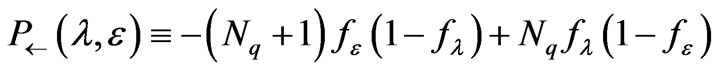
by a phonon with wave vector q and  means an electron transition from a state
  (distribution function:
![]() ) to a state
) to a state  (distribution function:
 ) with a phonon emission (distribution function:
 ) minus a transition from a state
  to a state
  with a phonon absorption
 . There is an another diagram connecting with a counterclockwise loop,
  , which is defined
 (4)
(4)
In a loop, the upper and lower half circles correspond to phonon emission ( ) and phonon absorption (
 ).
).
3) There are diagrams connecting the final state  to the implicit state
 ![]() with dotted line and connecting the implicit state
with dotted line and connecting the implicit state ![]() to a state
to a state  with a clockwise (or counterclockwise) loop. Figure 2 corresponds to clockwise loop.
4) Assign  for the clockwise loop
  , and assign
  for the counterclockwise loop
 . Here
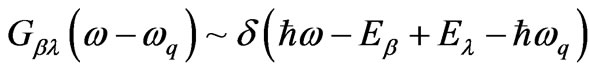
  called the G-factors are defined as follows:
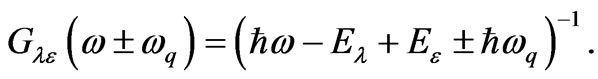 (5)
(5)
By , the energy conservation is satisfied, i.e.,
 .
.
5) Let the states connected to the dotted line involve no loops.
6) a) Multiply ,
,  , and
, and  for the clockwise loop. b) Multiply
 ,
,  , and
, and  for the counterclockwise loop.
7) Finally, sum all the diagrams after summing eachdiagram over all q and  values for the line shape function.
3. Linear Optical Conductivity
When an electromagnetic wave of frequency ![]() is applied to a system along the l (x, y, z) direction, the linear optical conductivity is given by the following: [10-12]
is applied to a system along the l (x, y, z) direction, the linear optical conductivity is given by the following: [10-12]
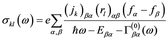 (6)
(6)
where  for electron states
 ![]() and
and , jk is the k component of the single electron current op-
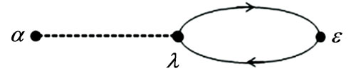
Figure 1. The dotted line and the clockwise loop correspond to  and
and , respectively.

Figure 2. The dotted line and the clockwise loop correspond to  and
and , respectively.
erator, rl is the l component of the electron position vector,  is the Fermi distribution function for an electron with energy
 , and
, and . Equation (6) can be represented by the diagram in Figure 3.
The energy term in Equation (6),
 , represents the transition from the initial state
 ![]() to the final state
to the final state  with a photon absorption of frequency
![]() . If there was no phonon scattering, the line shape would be like a delta function. However, as the electrons are scattered by phonons, the shape is broadened, so the line shape function
. If there was no phonon scattering, the line shape would be like a delta function. However, as the electrons are scattered by phonons, the shape is broadened, so the line shape function  is involved.
In Equation (6), there is no intermediate state between the initial state ![]() and final state
and final state , so the line shape function
  is represented by four loop diagrams in Figure 4.
From Figure 4,  is obtained as
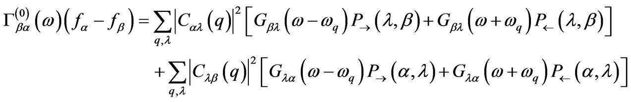 (7)
(7)
which is identical to the line shape function given by Equation (4.8) in [11].
The physical meaning of the first term in Equation (7) is as follows (see the first term in Figure 5). Since the absorption power delivered to the system is proportional to the real part of the conductivity [10,11],  becomes Dirac’s delta, i.e.,
 , since
 ![]() can be replaced by
can be replaced by  (
( ) in the response scheme.
Note that 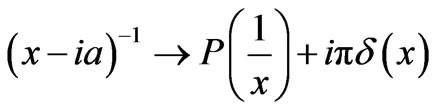 where P means principal value. Therefore,
  means that the implicit state
 ![]() is determined by the energy of the final state, photon energy, and phonon energy, so that energy conservation can be satisfied, i.e.
is determined by the energy of the final state, photon energy, and phonon energy, so that energy conservation can be satisfied, i.e. .
.  means that the implicit state
 ![]() is coupled with the initial state
is coupled with the initial state ![]() by a phonon with wave vector q.
by a phonon with wave vector q.  means that the reverse implicit transition from the final state
  to the intermediate state
 ![]() with phonon absorption should be subtracted from the forward implicit transition from the intermediate state
with phonon absorption should be subtracted from the forward implicit transition from the intermediate state ![]() to the final state
to the final state  with a phonon emission. This means that when an electron-phonon interaction is involved in the electron transition, there are local fluctuations, i.e. a transition occurs via implicit states. In other words, an electron undergoes a transition from the implicit state, which is coupled with the initial state, to the final state (or vice versa) with phonon emission (or absorption). The transition forms a loop because the absorption process maintains a balance with the emission process. Although
 ![]() is called the line shape function, the line shape must be calculated from Equation (6) not directly from Equation (7). Therefore, all the states given by
is called the line shape function, the line shape must be calculated from Equation (6) not directly from Equation (7). Therefore, all the states given by  are called the implicit states because they are included only in
![]() . Therefore, the transition from the initial state
. Therefore, the transition from the initial state ![]() to the final state
to the final state  occurs via two implicit transitions, and the implicit state is connected to the initial state by
  and to the final state by
 .
.
Although the implicit transitions are not measured directly, they should be considered in the calculations. Note that the other theories [1-7] cannot provide any diagram representation because they contain the sums of two distribution functions, such as 
The other three terms in  can be represented in a similar manner.
In Figure 4 or Equation (7), the first two terms are
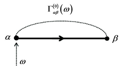
Figure 3. The transition from an initial state ![]() to a final state
to a final state ![]() with a photon absorption of frequency
with a photon absorption of frequency ![]() and a line shape function
and a line shape function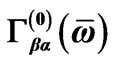 .
.
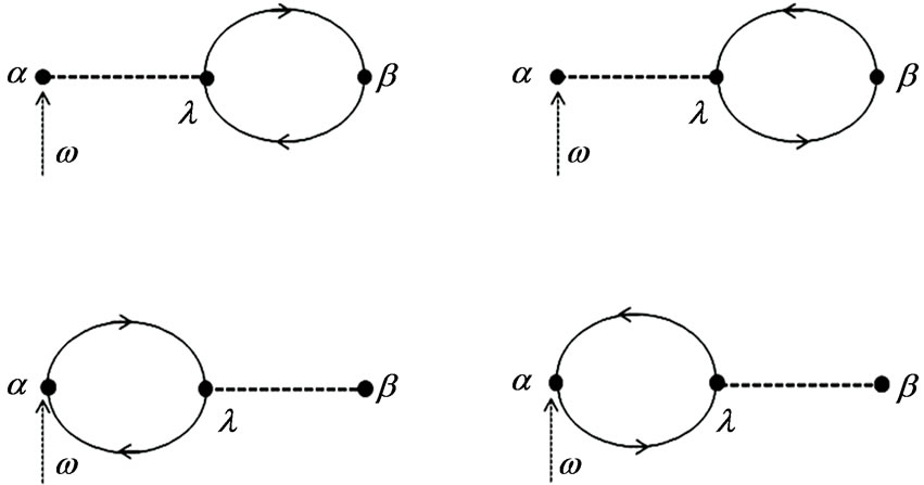
Figure 4. The dotted straight line means that the implicit state λ is coupled with the initial state α by a phonon in the first diagram. Two implicit transitions occur between the implicit state λ and final state β, which forms a loop. The other three diagrams can be interpreted in a similar manner.
topologically equivalent because the absorption of photons appears while phonons can be both absorbed and emitted in the transitions. The absorption (emission) of a photon or a phonon in the forward transitions is identical to the emission (absorption) in the reverse transitions, with negative contributions (minus signs) assigned to the reverse transitions. The final two terms are also topologically equivalent for the same reason. A net transition is possible because the implicit states are determined variously according to the energies of the final (or initial) state, photon energies, and phonon energies.
4. First-Order Nonlinear Optical Conductivity
The first-order nonlinear optical conductivity for two incident electromagnetic waves of frequencies  and
and  is given by the following [10-12]
 (8)
(8)
where . For the two photon process, there is an intermediate state
  between the initial state
 ![]() and final state
and final state . The first term in Equation (8) means thatthere is an intermediate transition from the intermediatestate
  to the final state
  with photon (
 ) absorption and line shape function
  and the direct transition from the initial state
 ![]() to the final state
to the final state  with two photons (
 ,
, ) absorption and line shape function
  (Figure 5). Note that
 .
.
 is called the intermediate state to be discerned from the implicit state because it is explicitly included in the conductivity but not in the line shape function.
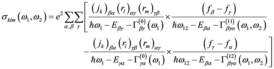
Four loop diagrams exist because there is an implicit state  between state
  and state
  through
  in the first term in Equation (8) (Figure 5). The first two terms involve
  in the
  transition of Figure 6, considering
  as a pseudo-
 state through
  and other two terms involve
  in the
  transition of Figure 5.
Therefore  can be expressed as follows:
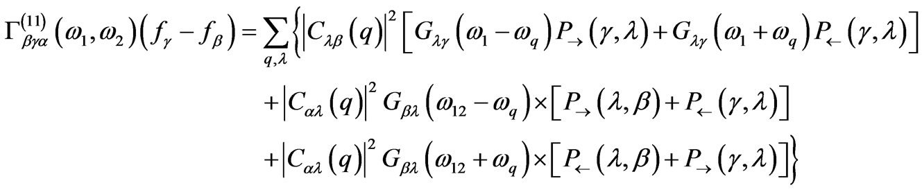 (9)
(9)
which is identical to the line shape function given by Equation (5.7) in [11]. The physical meaning of the third term in Equation (9) is as follows:  means that the implicit state
  is determined by the energy of the final state
 , two photon energies, and phonon energy; and
  means that the implicit state
  is coupledwith the initial state
 ![]() by a phonon with a wave vector q. There are two forward implicit transitions and two reverse implicit transitions with a center on the implicit state
by a phonon with a wave vector q. There are two forward implicit transitions and two reverse implicit transitions with a center on the implicit state . All the implicit states and types of phonons are included in the processes by the sums in Equation (9). The other three terms in
  can be interpreted in a similar manner. Similarly,
 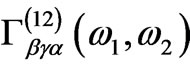 can be obtained. In Figure 6 or Equation (9), the first two terms and last two terms are topologically equivalent pairs for the same reason as in Figure 5 or Equation (7).
5. Concluding Remarks
In conclusion, this paper introduced a loop diagram approach to the nonlinear optical conductivity formula for an electron-phonon system. It was possible to explain the phonon emissions and absorptions in all electron transition processes in an organized manner because the line shape functions include the electron distribution functions properly as well as the phonon distribution functions. Since the present diagram method is not the one representing the trajectories of particles in the intermediate stages of scattering processes, these diagrams should not be confused with the time-ordered diagrams in the Feynman scheme [14] or with the temperature diagrams
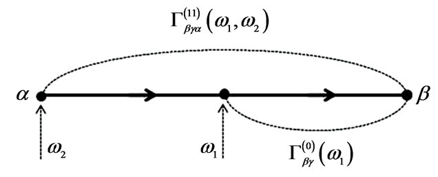
Figure 5. Two transition processes included in the first order nonlinear optical conductivity: 1) the intermediate transition from the intermediate state γ to the final state β with a photon ( ) absorption and the line shape function
  2) the transition from the initial state α to the final state β with two photons (
![]() ,
, ) absorption and the line shape function
 .
.
Figure 6. The dotted straight line means that the implicit state λ is coupled with the initial state α by a phonon in the third diagram. There are two forward implicit transitions and two reverse implicit transitions centered on the implicit state λ, which form loops. The other three diagrams can be interpreted in a similar manner.
in the Feynman-like scheme [15,16]. However, this method can be classified as another Feynman-like scheme, and shall be called the “KC loop diagrams” because all the contributions to the self-energy terms can be grouped into topologically-distinct loop diagrams based on the electron-phonon population topology originated by proper applications of KCRI’s and SDPO’s. This method can be applied further to other electron transition phenomena.
REFERENCES
- L. Hedin and S. Lundqvist, “In Solid State Physics,” Vol. 15, Academic, New York, 1969.
- G. Grimvall, “The Electron-Phonon Interaction in Metals,” North-Holland, New York, 1981.
- P.-B. Allen and B. Mitrovvich, “In Solid State Physics,” Vol. 37, Academic, New York, 1982.
- G. D. Mahan, “Many-Particle Physics,” Plenum, New York, 2000.
- B. Hellsing and S. Lundqvist, “Lifetime of Holes and Electrons at Metal Surfaces; Electron-Phonon Coupling,” Journal of Electron Spectroscopy and Related Phenomena, Vol. 129, No. 2-3, 2003, pp. 97-104. doi:10.1016/S0368-2048(03)00056-2
- F. Giustino, M. L. Cohen and S. G. Louie, “Small Phonon Contribution to the Photoemission Kink in the Copper Oxide Superconductors,” Nature, Vol. 452, 2008, pp. 975-978. doi:10.1038/nature06874
- A. Nechaev, I. Yu. Sklyadneva, V. M. Silkin, P. M. Echenique and E. V. Chulkov, “Theoretical Study of Quasiparticle Inelastic Lifetimes as Applied to Aluminum,” Physical Review B, Vol. 78, No. 8, 2008, Article ID 085113. doi:10.1103/PhysRevB.78.085113
- N. L. Kang, Y. J. Cho and S. D. Choi, “A Many-Body Theory of Quantum-Limit Cyclotron Transition LineShapes in Electron-Phonon Systems Based on Projection Technique,” Progress of Theoretical Physics, Vol. 96, No. 2, 1996, pp. 307-316. doi:10.1143/PTP.96.307
- N. L. Kang and S. D. Choi, “Scattering Effects of Phonons in Two Polymorphic Structures of Gallium Nitride,” Journal of Applied Physics, Vol. 106, No. 6, 2009, Article ID 063717. doi:10.1063/1.3226885
- H. J. Lee, N. L. Kang, J. Y. Sug and S. D. Choi, “Calculation of the Nonlinear Optical Conductivity by a Quantum-Statistical Method,” Physical Review B, Vol. 65, No. 19, 2002, Article ID 195113. doi:10.1103/PhysRevB.65.195113
- N. L. Kang and S. D. Choi, “Derivation of Nonlinear Optical Conductivity by Using a Reduction Identity and a State-Dependent Projection Method,” Journal of Physics A: Mathematical and Theoretical, Vol. 43, No. 16, 2010, p. 165203. doi:10.1088/1751-8113/43/16/165203
- N. L. Kang, Y. Lee and S. D. Choi, “Generalization of the Nonlinear Optical Conductivity Formalism by Using a Projection-Reduction Method,” Journal of Korean Physical Society, Vol. 58, No. 3, 2011, pp. 538-544. doi:10.3938/jkps.58.538
- N. L. Kang and S. D. Choi, “Validity of nth-Order Conductivity by the General Projection-Reduction Method,” Progress of Theoretical Physics, Vol. 125, No. 5, 2011, pp. 1011-1019. doi:10.1143/PTP.125.1011
- R. P. Feynman, “Space-Time Approach to Quantum Electrodynamics,” Physical Review, Vol. 76, No. 6, 1949, pp. 769-789. doi:10.1103/PhysRev.76.769
- L. Fetter and J. D. L. Walecka, “Quantum Theory of Many-Particle Systems,” McGraw Hill, New York, 1971.
- R. D. Mattuch, “A Guide to Feynman Diagrams in the Many-Body Problem,” 2nd Edition, McGraw-Hill, New York, 1976.