Applied Mathematics
Vol.5 No.10(2014), Article
ID:46594,8
pages
DOI:10.4236/am.2014.510151
On q-Deformed Calculus in Quantum Geometry
Olaniyi S. Maliki1, Emmanuel I. Ugwu2
1Department of Industrial Mathematics and Applied Statistics, Ebonyi State University, Abakaliki, Nigeria
2Department of Industrial Physics, Ebonyi State University, Abakaliki, Nigeria
Email: somaliki@yahoo.com, ugwuei@yahoo.com
Copyright © 2014 by authors and Scientific Research Publishing Inc.
This work is licensed under the Creative Commons Attribution International License (CC BY).
http://creativecommons.org/licenses/by/4.0/


Received 21 March 2014; revised 21 April 2014; accepted 28 April 2014
ABSTRACT
The relation between noncommutative (or quantum) geometry and the mathematics of spaces is in many ways similar to the relation between quantum physics and classical physics. One moves from the commutative algebra of functions on a space (or a commutative algebra of classical observable in classical physics) to a noncommutative algebra representing a noncommutative space (or a noncommutative algebra of quantum observables in quantum physics). The object of this paper is to study the basic rules governing q-calculus as compared with the classical NewtonLeibnitz calculus.
Keywords:Quantum Geometry, q-Numbers, q-Factorials, q-Calculus

1. Introduction
There exists an intimate relationship between classical geometry and physics, and to appreciate this we will consider the Einstein field equations (EFE) of special relativity written as:
 (EFE)
(EFE)
where  is the Einstein tensor,
  is the Ricci tensor.
  is the energy-momentum tensor.
For the moment we are only interested in three basic properties of the above equation.
1) The equation (EFE) is a tensor equation. This is necessarily so, since the principle of invariance under coordinate transformations must hold, in other words the equations of physics must look the same in any frame of reference.
2) We can interpret equation (EFE) more simply as

i.e. it is the presence of matter in space that distorts the neighbouring geometry. Most equations of mathematical physics can be interpreted similarly.
3) The solution to equation (EFE) is a geometrical object, namely a line element given by

where  is the metric tensor to be solved for in (EFE).
1.1. Quantum Geometry
Every geometry is associated with some kind of space. Quantum (or noncommutative) geometry [1] [2] deals with quantum spaces, including the classical concept of space as a very special case. In classical geometry spaces are always regarded as collections of points equipped with the appropriate additional structure (as for example a topological structure given by the collection of open sets, or a smooth structure given by the atlas). In contrast to classical geometry, quantum spaces are not interpretable in this way. In general, quantum spaces have no points at all! They exhibit non-trivial quantum fluctuations’ of geometry at all scales.
In generalizing classical geometry to the non-commutative level, there are two important conceptual steps:
1) Translation of geometry into a commutative algebra format;
2) Non-commutative generalizations.
1.2. Reformulating Basic Geometrical Concepts
It turns out that the geometrical structure on any given topological space X is always completely expressible in the language of some associated *-algebra [3] [4] .
Points
Let X be a compact topological space, and let be the *-algebra of continuous complex-valued functions on X. Every element
  naturally gives rise to a linear functional
  defined by
This map is multiplicative in the sense that

Furthermore,  is Hermitian in the sense that
  it is also non-zero, i.e.
  is a character on A. Conversely, consider an arbitrary character
 , then it can be shown that there exists a unique point
  such that
 . In other words, we have a natural bijection between points of X and characters of A. It is important to note that this characterization of points also remains valid at the smooth level, in which X could be a compact smooth manifold and the associated *-algebra consists of smooth functions on X.
1.3. The Gelfand-Naimark Theorem
The algebra  of complex-valued functions on a compact topological space X, equipped with the maximum norm

is a commutative C*-algebra [2] . The classical theorem of Gelfand and Naimark characterizes the algebras of the form , as commutative unital C*-algebras. This means that for every commutative unital C*-algebra A there exists (up to homeomerphisms) a unique compact topological space X such that
 .
.
As we have earlier observed, the points of the space X are recovered as characters of the associated algebra A. In terms of this identification, the topology on X coincides with the weak*-topology, induced from the dual space , consisting of continuous linear functionals on A. It turns out that homomorphisms between C*-algebras are automatically continuous, in particular characters are continuous linear functionals.
2. The Quantum Plane
A simple example of quantum geometry is the quantum plane (Figure 1). Usually, a plane is described by two coordinate functions x, y. Naturally, the functions xy and yx are the same since it does not matter whether you measure x first and then y or y first and then x. This is precisely what is lost in the quantum world.
In the quantum plane we replace the property  by
by  where q is some parameter. We no longer have points, however we can continue to work algebraically with x and y.
Define , the commutator bracket. Hence
  can be rewritten as

The commutative case is obtained when .
.
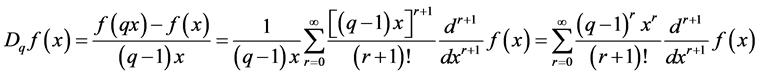
2.1. q-Deformed Calculus
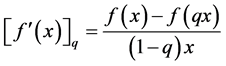
It is interesting to know that one can really do geometry in this setting, where coordinates do not commute. This is the remarkable discovery in recent times. For example, we can follow the approach of Newton-Leibnitz defining differentiation by

But when  and in particular
  we get instead
Thus for example the derivative of the function  in this non-commutative setting would be
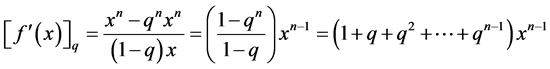
We observe here that when  the derivative of
  for the commutative case is obtained, i.e.
 .
.
2.2. Basic Notions of q-Calculus
The mathematical study of noncommutative geometry is intimately related to the so-called q-calculus (qnumbers, q-factorials, q-differentials and integrals, basic q-hypergeometric functions, and q-orthogonal polynomials). Here we give a brief introduction to q-numbers and q-factorials which will be required in the subsequent sections.
2.2.1. q-Numbers and q-Factorials
For any nonzero complex number q, the q-number , is defined by
 (2.1)
(2.1)
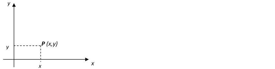
Figure 1. The quantum plane (xy ≠ yx).
We observe that, . The following expression which is easily proved will prove useful.
 (2.2)
(2.2)
Thus given , as shown previously
 .
.
2.2.2. Proposition
The q-numbers satisfy the following relations derived from the property of the exponential function 1) 
2) 
3) 
4) 
5) 
The proof of 1) is easy to see from the fact that;

Let 
Hence;

The rest of the identities can be proved similarly. It is important to note that the relations 1)-5) remain valid when q is considered an indeterminate. Consequently any q-number , belongs to the space
 of Laurent polynomials [2] in q with integral coefficients.
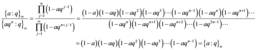
Suppose , then we define the q-factorial
  by setting;

The following expression is quite useful in the theory of hypergeometric functions as well as in combinatorics.
 (2.3)
(2.3)
It is now possible for us to relate the above with the q-factorials. We observe that;
 (2.4)
(2.4)
From equation (2.3) we note that  For
For , define
 (2.5)
(2.5)
which converges , and defines an analytic function on
 .
.
2.2.3. Proposition
 ,
,  ,
, .
.
Proof
Remark: We can also define and show that;
 (2.6)
(2.6)
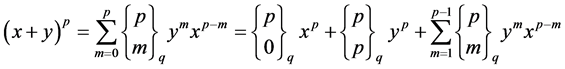
2.2.4. q-Binomial Coefficients
The q-binomial coefficients are defined by the formula;
 (2.7)
(2.7)
Remark: There exist a close analogy between the classical binomial coefficients  and their q-analogues. Many of the identities satisfied by the former have their counterparts for the q-binomial coefficients. For example the classical identity;

simply translates to;
 2.8
2.8
2.2.5. Proposition
Let  and
and  be noncommuting variables satisfying the relation
 , then we have
 (2.9)
(2.9)
In case q is a primitive pth root of unity, and p is odd, then
 (2.10)
Proof
Equation (2.9) can be established by induction on n, and employing the first identity in (2.8). The second assertion follows directly from (2.9). Observe that:
From (2.7)

and .
.
3. q-Differential and q-Integral Operators
The following are important basic notions derived from their analogue in classical calculus, and will be employed subsequently.
3.1. The q-Differential Operator
For , we define the q-differential operator
  by:
by:
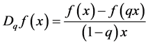 (3.1)
(3.1)
Note that  as
as .
.
Proposition:
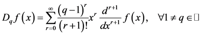 . (3.2)
Provided the expression on the right hand side exists.
Proof
Let , then by Taylor’s series,

Setting , we have:
The formula for the product of two functions is given by

We can now define the q-analogue of the Newton-Leibnitz rule:
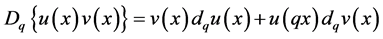 (3.3)
(3.3)
Thus,
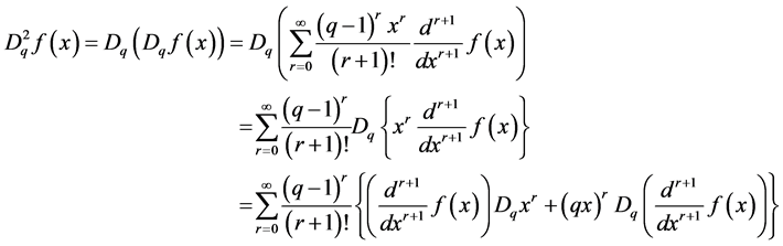
By induction on n, it follows from (3.3) that:
 (3.4)
(3.4)
As a special case when ,
,  is evaluated to give:
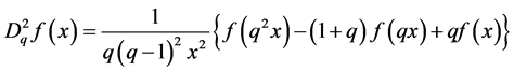 (3.5)
(3.5)
3.2. The q-Integral Operator
The q-integral operator will be defined as the inverse of the q-differential operator.
Given , we have:
 (3.6)
(3.6)
It then follows that; .
.
Hence, summing these relations over  gives:
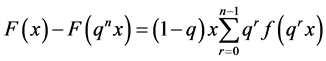 (3.7)
(3.7)
Assuming  so that
  as
as , it follows that
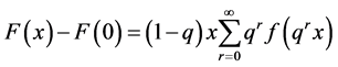
We can now formally define the q-integral of a function  on a given interval
  as
as
 (3.8)
(3.8)
On the semi-infinite interval , the q-integral of a function
  is defined as:
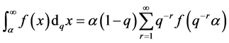 (3.9)
(3.9)
Over any closed interval , the q-integral of a function
  is given by
 (3.10)
We now define the integral over the interval . This is achieved by setting
  in equations (3.8) and (3.9) and summing to get:
 (3.11)
The integration by parts formula of Newton-Leibnitz calculus is interpreted in the present noncommutative context as:

4. Application
There are a number of applications of the foregoing, we mention here just two, namely:
1) q-binomial formulae in two variables satisfying a quadratic relation, this has recently been published in [5] and [6] . These relations have applications in quantum group theory and non-commutative geometry.
2) A recent trend in modern physics is the study of the quantum anti-de Sitter space [7] [8] possibly in connection with q = root of unity [9] .
Acknowledgements
This work began at the African Institute for mathematical sciences (AIMS) in Muizenberg South Africa, when the first author visited in 2010. I wish to thank the director Prof Fritz Hahne for giving me a postdoctoral fellowship, and for providing a conducive environment which made this research possible.
References
- Connes, A. (1986) Non-Commutative Differential Geometry. Extrait des Publications Mathematiques-IHES, 62. (cited in: Qauntum Principal Bundles and Their Characteristic Classes (pdf), by MICO DURDEVIC, arXiv:q-alg/960505008vi (5 May 1996))
- Connes A. (1994) Noncommutative Geometry. Academic Press New York.
- Brateli O. and Robinson, D. (1979) Operator Algebras and Quantum Statistical Mechanics, Volumes 1/2. SpringerVerlag, Berlin.
- Brown L.G., Douglas, R.G. and Filmore, P.G. (1977) Extensions of C*-Algebras and K-Homology. Annals of Mathematics, 105, 265-324. http://dx.doi.org/10.2307/1970999
- Benaoum H.B. (1999) (q; h)-Analogue of Newton’s Binomial Formula. Journal of Physics A: Mathematical and General, 32, 2037-2040. http://dx.doi.org/10.1088/0305-4470/32/10/019
- Rosengren H. (1999) Multivariable Orthogonal Polynomials as Coupling Coefficients for Lie and Quantum Algebra Representations. Dissertation, Centre for Mathematical Sciences, Mathematics (Faculty of Science), Lund, 167.
- Kowalski-Glikman J. (1998) Black Hole Solution of Quantum Gravity. Physics Letters A, 250, 62-66. http://dx.doi.org/10.1016/S0375-9601(98)00706-3
- Chang Z. (1999) Quantum Anti-De Sitter Space. (reprint)
- Steinacker H. (1998) Finite Dimensional Unitary Representations of Quantum Antide Sitter Groups at Roots of Unity. Communications in Mathematical Physics, 192, 687-706. http://dx.doi.org/10.1007/s002200050315