Applied Mathematics
Vol. 4 No. 2 (2013) , Article ID: 28420 , 7 pages DOI:10.4236/am.2013.42061
Wavelet Density Estimation and Statistical Evidences Role for a GARCH Model in the Weighted Distribution
Department of Statistics, Ferdowsi University of Mashhad, Mashhad, Iran
Email: abbaszadeh.mo@stu-mail.um.ac.ir, emadi@um.ac.ir
Received November 10, 2012; revised December 10, 2012; accepted December 17, 2012
Keywords: Density Estimation; GARCH Model; Weighted Distribution; Wavelets; Statistical Evidences; Strongly Mixing
ABSTRACT
We consider n observations from the GARCH-type model: Z = UY, where U and Y are independent random variables. We aim to estimate density function Y where Y have a weighted distribution. We determine a sharp upper bound of the associated mean integrated square error. We also make use of the measure of expected true evidence, so as to determine when model leads to a crisis and causes data to be lost.
1. Introduction
We suppose that  is a sample of a strictly stationary and exponentially strongly mixing process
  where, for any
 ,
,
 (1)
(1)
 is a sequence of identically distributed random variables with common known density
  and
and  is a sequence of identically distributed random variables with common unknown density
 . For any
 ,
,  and
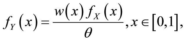
and ![]() are independent. We suppose that
are independent. We suppose that  is a weighted density of the form
 (2)
(2)
where ![]() is a known positive function,
is a known positive function,  an unknown density of a random variable
  and
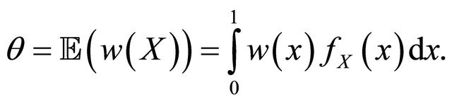
and  is the unknown normalization parameter:
Our goal is to estimate  when only
  are observed. The Equation (1) is a GARCH-type time series model classically encountered in financial models see [1] and practical examples of Equation (2) can be found in e.g. [2-4].
In this article, we construct a linear wavelet estimator and measure its performance by determining upper bounds of the mean integrated squared error (MISE) over Besov space.
In what follows, we have also surveyed the role of data and evidential inference in the model. The data play a very important essential role in statistical analysis, to the extent that many statistical researchers believe in the famous saying: “Ask the data.” We consider the Test
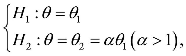 (3)
(3)
for the model and we evaluate the sensitivity of the value in the test hypotheses. In this test, the evaluation criterion is the area between the curves of the cumulative distribution functions under  and
and  hypotheses. Details on evidential inference can be found in [5,6]. Also [7] have studied about Comparing of record data and random observation based on statistical evidence.
Through the rest of the paper, at first assumptions and then an introduction about wavelets are presented in Section 2. The estimators and results are given in Section 3. In Section 4, general explanations regarding evidential inference and its application in a test. The proofs are gathered in Section 5.
2. Assumptions and Wavelets
2.1. Assumptions
We formulate the following assumptions:
• Without loss of generality, we assume that  and
and
 have the support
  and
and  where
where
• 
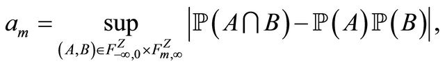
• We suppose that for any , the
, the ![]() -th strongly mixing coefficient of
-th strongly mixing coefficient of  by
by
where, for any , let
, let  be the
 ![]() -algebra generated by
-algebra generated by  and
and  is the
 ![]() -algebra generated by
-algebra generated by .
.
We suppose that there exist three (known) constants,  and
and  such that
This assumption is satisfied by a large class of GARCH processes. See e.g. [8-10].
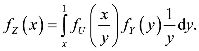
• For any , it follows from the independence of
  and
and ![]() that the density of
that the density of  is
is
• 
• We suppose that there exists two constants,  and
and , such that
 (4)
(4)
and
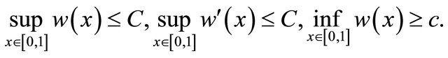 (5)
(5)
2.2. Wavelets and Besov Balls
Let  be a positive integer, and
  and
and  be the Daubechies wavelets
  which satisfy
 .
.
Set
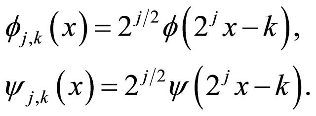
Then, there exists an integer ![]() such that, for any integer
such that, for any integer , the collection
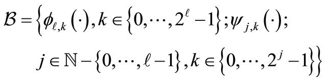
is an orthonormal basis of  (the space of squareintegrable functions on 0,1). We refer to [11].
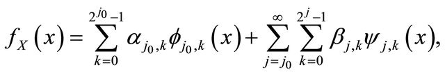
For any integer , any
, any  can be expanded on
  as
as
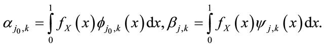
where  and
and  are the wavelet coefficients of
  defined by
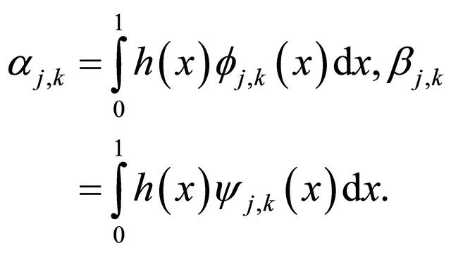 (6)
(6)
Let  and
and . A function
  belongs to
  if and only if there exists a constant
  (depending on
 ) such that the associated wavelet coefficients Equation (6) satisfy
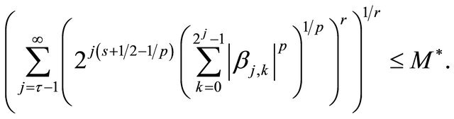
We set . Details on Besov balls can be found in [12].
3. Estimators and Results
Firstly, we consider the following estimator for 
 (7)
(7)
Then, for any integer  and any
 , we estimate
 (8)
(8)
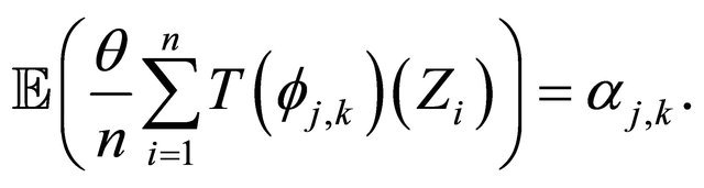
where, for any ,
, ![]() is the operator
is the operator
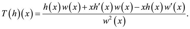 (9)
(9)
 and
and  are similar with multiplicative censoring model (see [13]).
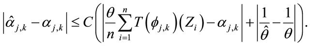
We are now in the position to define the considered estimators for . Suppose that
 . We define the linear estimator
  by
by
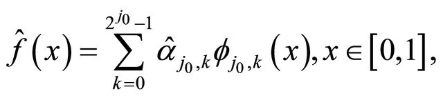 (10)
(10)
where  is defined by Equation (8) and
  is the integer satisfying
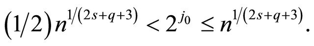 (11)
(11)
• Lemma 3.1
• Let  be Equation (7) and
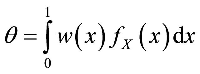 . Then we have
• 
• Let  be Equation (1),
 ![]() be Equation (9) and for any integer
be Equation (9) and for any integer  and any
 ,
,
 . Then we have
• 
• For any integer  and any
 , let
, let
 be Equation (8) and
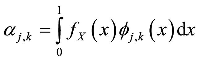 .
.
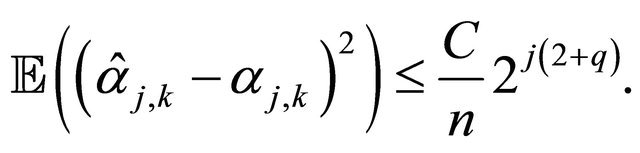
Then, under the assumptions of Subsection 2.1, there exists a constant  such that
Proposition 3.1 For any integer  and any
  Then, under the assumptions of Subsection 2.1•

Proposition 3.2 Let , for any integer
  and any
 , let
, let  be Equation (8) and
 . Then• there exists a constant
  such that
• 
• there exists a constant  such that
• 
• there exists a constant  such that
Theorem 3.1 (Upper bound for ) Consider Equation (1) under the assumptions of Subsection 2.1. Suppose that
  with
with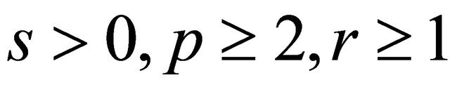 . For any
 and
and  be Equation (10), then there exists a constant
  such that
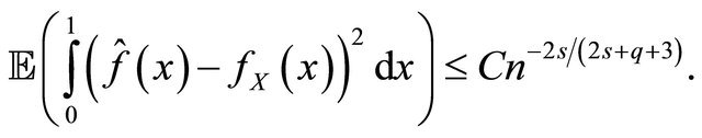
Remark that  is the slower than the optimal one in the standard density estimation problem i.e.
  (see e.g. [14, Chapter 10]). This deterioration is due to the presence of GARCH model and weighted distribution.
4. Statistical Evidence
4.1. Statistical Inference
The evidential approach to statistical inference concerns a novel approach in statistical analysis. Evidential inference is solely based on data as evidence and calculation of the evidence strength. It is not influenced by mental and personal components and factors such as former beliefs and loss functions. Using evidential inference in the model Equation (1), we will survey when censoring of data will lead to considerable data loss, and we will determine the time when data is lost by determining an appropriate criterion. In the model for
for , the data observed from the variable
  are denoted by the subscript (cen), and the data observed from the variable
 ![]() are denoted by the subscript (ncen). Considering the Test Equation (3) in the above model, due to the symmetry of the test hypotheses in evidential methods and without losing the generality of the problem, the value of is assumed to be
are denoted by the subscript (ncen). Considering the Test Equation (3) in the above model, due to the symmetry of the test hypotheses in evidential methods and without losing the generality of the problem, the value of is assumed to be . In order to support
  and
and  hypotheses, we now use the following criterion:
 (12)
(12)
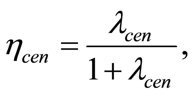
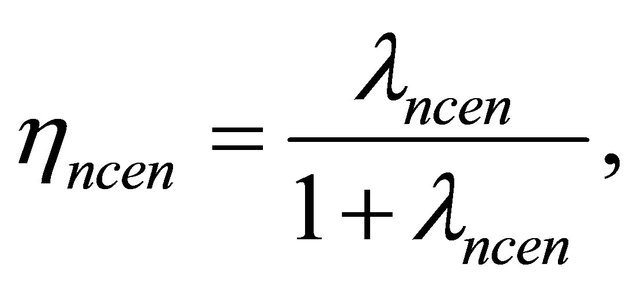
where  and
and  are the measure of expected true evidence in the censored and uncensored data respectively, and
  is the criterion of the support of data from
  hypothesis against
  hypothesis. This support criterion is optimal when the area between the two curves of
  cumulative functions under
  and
and  is maximum, please see [15]. This area which is denoted by
  in the form of
where  is the cumulative distribution function of
  and
and  is the mean value of
  under
under  hypotheses. In view of [6], the support criterion
  is defined as follows:
 (13)
(13)
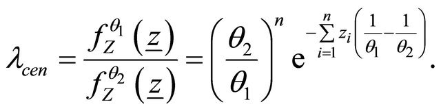
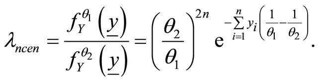
where ![]() is the likelihood ratio and for the two censored and uncensored cases we have
is the likelihood ratio and for the two censored and uncensored cases we have
 (14)
(14)
where  and
and  are likelihood functions for
  and
and ![]() variables respectively, in the Equation (1) under
variables respectively, in the Equation (1) under  hypotheses.
4.2. Measuring Statistical Evidence
We consider i.i.d case for variables in the Equations (1) and (2), also set  and then, we investigate the behavior of
 ![]() by means of simulation. In addition, we analyze
by means of simulation. In addition, we analyze  and
and  hypotheses in Test Equation (3) by determining support criterion
  of the measure of expected true evidence
 . The programming codes of this part are written in the MAPLE (15) environment.
Example 1. In this example, we generate data from gamma and uniform distribution as follows, considering multiplicative censoring model:
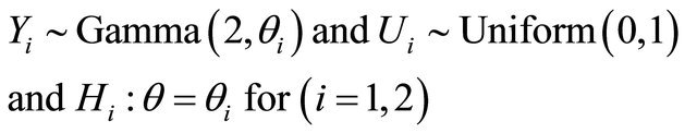
Then, according to Equations (13) and (14), we calculate the support criterion and the likelihood ratio via below relations:
such that
and
such that
For different values of ![]() and
and![]() , we calculate the value of
, we calculate the value of  according to Equation (12). The results can be observed in Table 1. By carefully considering this table, it is observed that as the value of
 ![]() increases (which implies the distance growth between
increases (which implies the distance growth between  and
and ), the value of
  gets closer to one. In other words,
  approaches
  more and more. This fact can be interpreted in this way that if the distance between
  and
and  is large, the data lost in censored data
 ![]() is negligible. That is to say, evidential inference draws our attention to the time when
is negligible. That is to say, evidential inference draws our attention to the time when  is close to
 . The above analysis can also be observed in Figure 1.
In what follows, the variations of sample volume ratio increase against ![]() are investigated, and the value of
are investigated, and the value of
![]() in the
in the  equation is determined for different values of
  and
and .
.
If  then
then . The result can be viewed in Figure 2, If
  then
then . The result can be viewed in Figure 3, If
then . The result can be viewed in Figure 4.
The above results can be interpreted in this way that as the sample volume increases from a certain stage on, the value of ![]() remains constant. In other words, it can be intuitively said that the
remains constant. In other words, it can be intuitively said that the  ratio tends to the constant
 ![]() value, which this also leads to an increase in evidential strength.
value, which this also leads to an increase in evidential strength.
5. Proofs
In this section,  denotes any constant that does not depend on
  and
and![]() . Its value may change from one term to another and may depends on
. Its value may change from one term to another and may depends on  or
or .
.
Table 1. Computed values for γ.
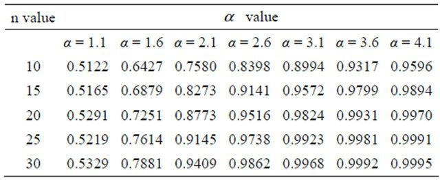
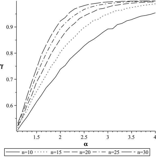
Figure 1. γ computed from gamma distribution for different values of n.
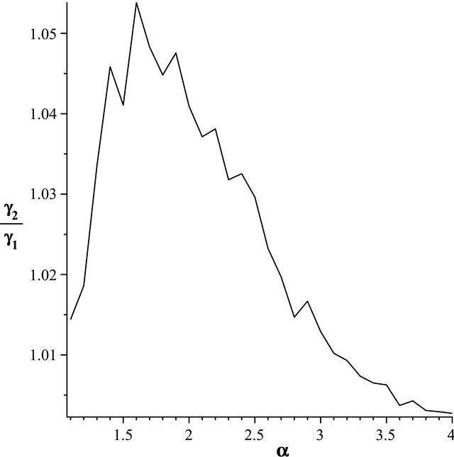
Figure 2. The most relative changes when sample size n1 = 20 increases to n2 = 25 happens in α = 1.6.

Figure 3. The most relative changes when sample size n1 = 10 increases to n2 = 15 happens in α = 2.1.
Proof of Lemma 3.1.
Proof can be found in [13].
Proof of proposition 3.1.
1. By Equation (9) and Equation (5), we have
 (15)
(15)
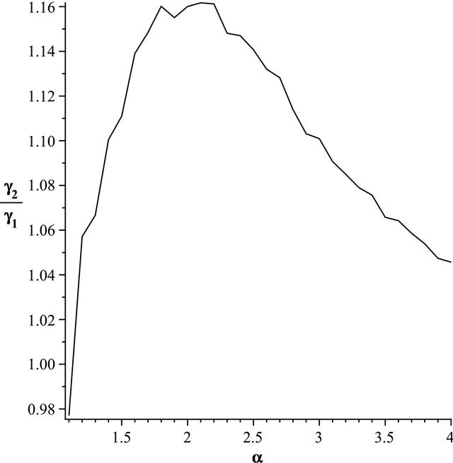
Figure 4. The most relative changes when sample size n1 = 10 increases to n2 = 20 happens in α = 2.2.
Therefore
 (16)
(16)
2. By Equation (9) and Equation (5), we have
 (17)
(17)
By Equation (4) and under the assumptions of Subsection 2.1 and also doing the change of variables , we have
 (18)
(18)
Using again Equation (4) and the assumptions of Subsection 2.1, the equality 
and doing the change of variables , we obtain
 (19)
(19)
Combining Equations (17)-(19), we obtain
 (20)
(20)
The proof of Proposition 3.1 is complete.
Proof of Proposition 3.2.
1. We have
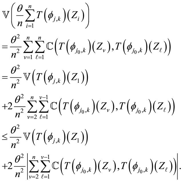 (21)
(21)
Using Equation (20) we obtain
 (22)
(22)
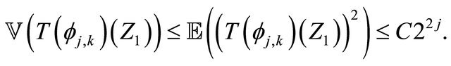
also
 (23)
(23)
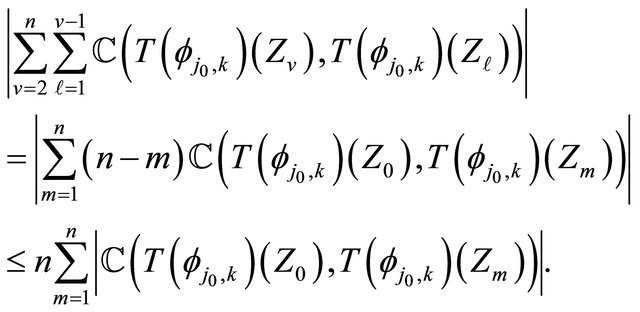
By the Davydov inequality (see [16]) and for any  we obtain
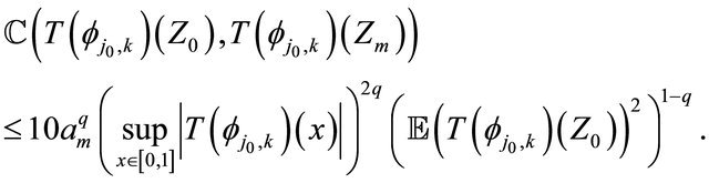 (24)
(24)
Putting Equation (24), Equation (16) and Equation (20) together, we have
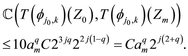 (25)
(25)
Since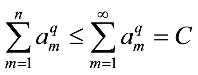 , we obtain
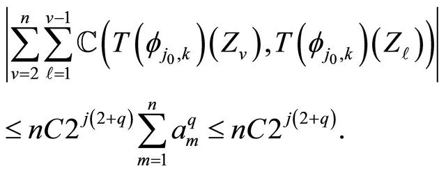 (26)
(26)
Putting Equations (21) and (22) and Equation (26) together, we have
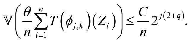 (27)
(27)
2. We have
 (28)
(28)
By Equation (5), we have
 (29)
(29)
By the Davydov inequality (see [16]) we obtain
 (30)
(30)
Combining Equations (28)-(30), we obtain
 (31)
(31)
3. Using Lemma (3.1), Equation (27) and Equation (31), then
 (32)
(32)
The proof of Proposition 3.2 is complete.
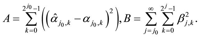
Proof of Theorem 3.1. For any integer , any
, any  can be expanded on
  as
as
where
We obtain
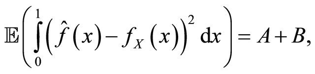
where
Using Proposition 3.2 and inequalitity Equation (11)
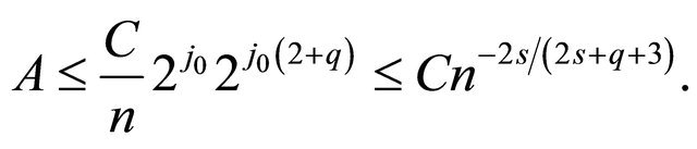
and since , we have
 . Hence
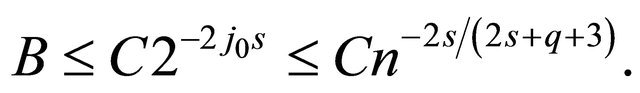
Hence we have

This ends the proof of Theorem 3.1.
REFERENCES
- M. Carrasco and X. Chen, “Mixing and Moment Properties of Various GARCH and Stochastic Volatility Models,” Econometric Theory, Vol. 18, No. 1, 2002, pp. 17-39. doi:10.1017/S0266466602181023
- S. T. Buckland, D. R. Anderson, K. P. Burnham and J. L. Laake, “Distance Sampling: Estimating Abundance of Biological Populations,” Chapman and Hall, London, 1993.
- D. Cox, “Some Sampling Problems in Technology,” In: N. L. Johnson and H. Smith Jr., Eds., New Developments in Survey Sampling, Wiley, New York, 1969, pp. 506-527.
- J. Heckman, “Selection Bias and Self-Selection,” The New Palgrave: A Dictionary of Economics, MacMillan Press, Stockton, 1985, pp. 287-296.
- R. Royall, “Statistical Evidence,” A Likelihood Paradigm, Chapman and Hall, London, 1997.
- R. Royall, “On the Probability of Observing Misleading Statistical Evidence,” Journal of the American Statistical Association, Vol. 95, No. 451, 2000, pp. 760-780. doi:10.1080/01621459.2000.10474264
- M. Emadi, J. Ahmadi and N. R. Arghami, “Comparing of Record Data and Random Observation Based on Statistical Evidence,” Statistical Papers, Vol. 48, No. 1, 2007, pp. 1-21. doi:10.1007/s00362-006-0313-z
- C. Chesneau and H. Doosti, “Wavelet Linear Density Estimation for a GARCH Model under Various Dependence Structures,” Journal of the Iranian Statistical Society, Vol. 11, No. 1, 2012, pp. 1-21.
- P. Doukhan, “Mixing Properties and Examples,” Lecture Notes in Statistics 85, Springer Verlag, New York, 1994.
- D. Modha and E. Masry, “Minimum Complexity Regression Estimation with Weakly Dependent Observations,” IEEE Transactions on Information Theory, Vol. 42, No. 6, 1996, pp. 2133-2145. doi:10.1109/18.556602
- A. Cohen, I. Daubechies, B. Jawerth and P. Vial, “Wavelets on the Interval and Fast Wavelet Transforms,” Applied and Computational Harmonic Analysis, Vol. 24, No. 1, 1993, pp. 54-81. doi:10.1006/acha.1993.1005
- Y. Meyer, “Wavelets and Operators,” Cambridge University Press, Cambridge, 1992.
- M. Abbaszadeh, C. Chesneau and H. Doosti, “Nonparametric Estimation of Density under Bias and Multiplicative Censoring via Wavelet Methods,” Statistics and Probability Letters, Vol. 82, No. 5, 2012, pp. 932-941. doi:10.1016/j.spl.2012.01.016
- W. Härdle, G. Kerkyacharian, D. Picard and A. Tsybakov, “Wavelet, Approximation and Statistical Applications,” Lectures Notes in Statistics, Springer Verlag, New York, 1998, Vol. 129.
- M. Emadi and N. R. Arghami, “Some Measure of Support for Statistical Hypotheses,” Journal of Statical Theory and Applications, Vol. 2, No. 2, 2003, pp. 165-176.
- Y. Davydov, “The Invariance Principle for Stationary Processes,” Theory of Probability & Its Applications, Vol. 15, No. 3, 1970, pp. 498-509. doi:10.1137/1115050