Paper Menu >>
Journal Menu >>
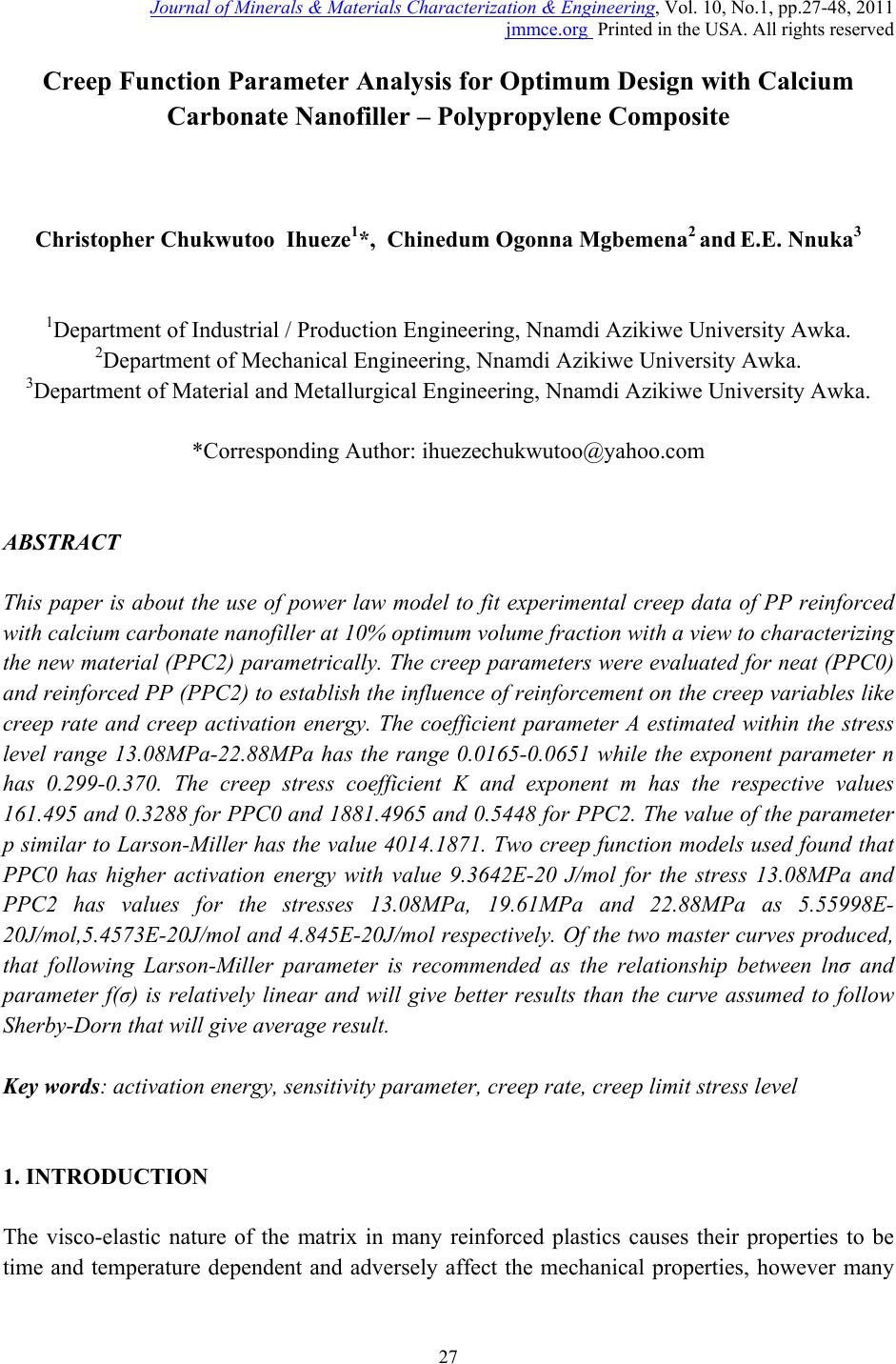 Journal of Minerals & Materials Characterization & Engineering, Vol. 10, No.1, pp.27-48, 2011 jmmce.org Printed in the USA. All rights reserved 27 Creep Function Parameter Analysis for Optimum Design with Calcium Carbonate Nanofiller – Polypropylene Composite Christopher Chukwutoo Ihueze1*, Chinedum Ogonna Mgbemena2 and E.E. Nnuka3 1Department of Industrial / Production Engineering, Nnamdi Azikiwe University Awka. 2Department of Mechanical Engineering, Nnamdi Azikiwe University Awka. 3Department of Material and Metallurgical Engineering, Nnamdi Azikiwe University Awka. *Corresponding Author: ihuezechukwutoo@yahoo.com ABSTRACT This paper is about the use of power law model to fit experimental creep data of PP reinforced with calcium carbonate nanofiller at 10% optimum volume fraction with a view to characterizing the new material (PPC2) parametrically. The creep parameters were evaluated for neat (PPC0) and reinforced PP (PPC2) to establish the influence of reinforcement on the creep variables like creep rate and creep activation energy. The coefficient parameter A estimated within the stress level range 13.08MPa-22.88MPa has the range 0.0165-0.0651 while the exponent parameter n has 0.299-0.370. The creep stress coefficient K and exponent m has the respective values 161.495 and 0.3288 for PPC0 and 1881.4965 and 0.5448 for PPC2. The value of the parameter p similar to Larson-Miller has the value 4014.1871. Two creep function models used found that PPC0 has higher activation energy with value 9.3642E-20 J/mol for the stress 13.08MPa and PPC2 has values for the stresses 13.08MPa, 19.61MPa and 22.88MPa as 5.55998E- 20J/mol,5.4573E-20J/mol and 4.845E-20J/mol respectively. Of the two master curves produced, that following Larson-Miller parameter is recommended as the relationship between lnσ and parameter f(σ) is relatively linear and will give better results than the curve assumed to follow Sherby-Dorn that will give average result. Key words: activation energy, sensitivity parameter, creep rate, creep limit stress level 1. INTRODUCTION The visco-elastic nature of the matrix in many reinforced plastics causes their properties to be time and temperature dependent and adversely affect the mechanical properties, however many 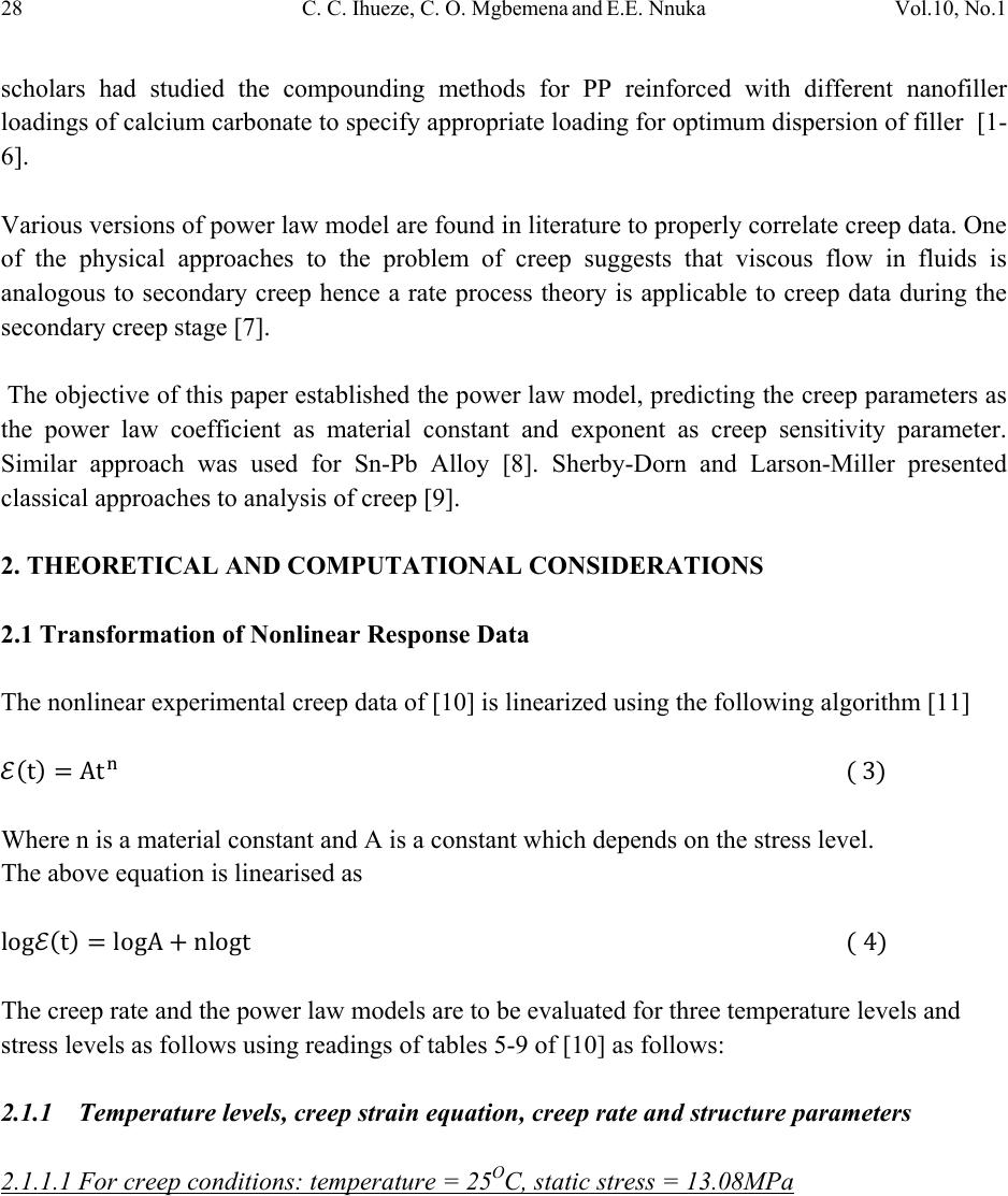 28 C. C. Ihueze, C. O. Mgbemena and E.E. Nnuka Vol.10, No.1 scholars had studied the compounding methods for PP reinforced with different nanofiller loadings of calcium carbonate to specify appropriate loading for optimum dispersion of filler [1- 6]. Various versions of power law model are found in literature to properly correlate creep data. One of the physical approaches to the problem of creep suggests that viscous flow in fluids is analogous to secondary creep hence a rate process theory is applicable to creep data during the secondary creep stage [7]. The objective of this paper established the power law model, predicting the creep parameters as the power law coefficient as material constant and exponent as creep sensitivity parameter. Similar approach was used for Sn-Pb Alloy [8]. Sherby-Dorn and Larson-Miller presented classical approaches to analysis of creep [9]. 2. THEORETICAL AND COMPUTATIONAL CONSIDERATIONS 2.1 Transformation of Nonlinear Response Data The nonlinear experimental creep data of [10] is linearized using the following algorithm [11] Where n is a material constant and A is a constant which depends on the stress level. The above equation is linearised as The creep rate and the power law models are to be evaluated for three temperature levels and stress levels as follows using readings of tables 5-9 of [10] as follows: 2.1.1 Temperature levels, creep strain equation, creep rate and structure parameters 2.1.1.1 For creep conditions: temperature = 25OC, static stress = 13.08MPa 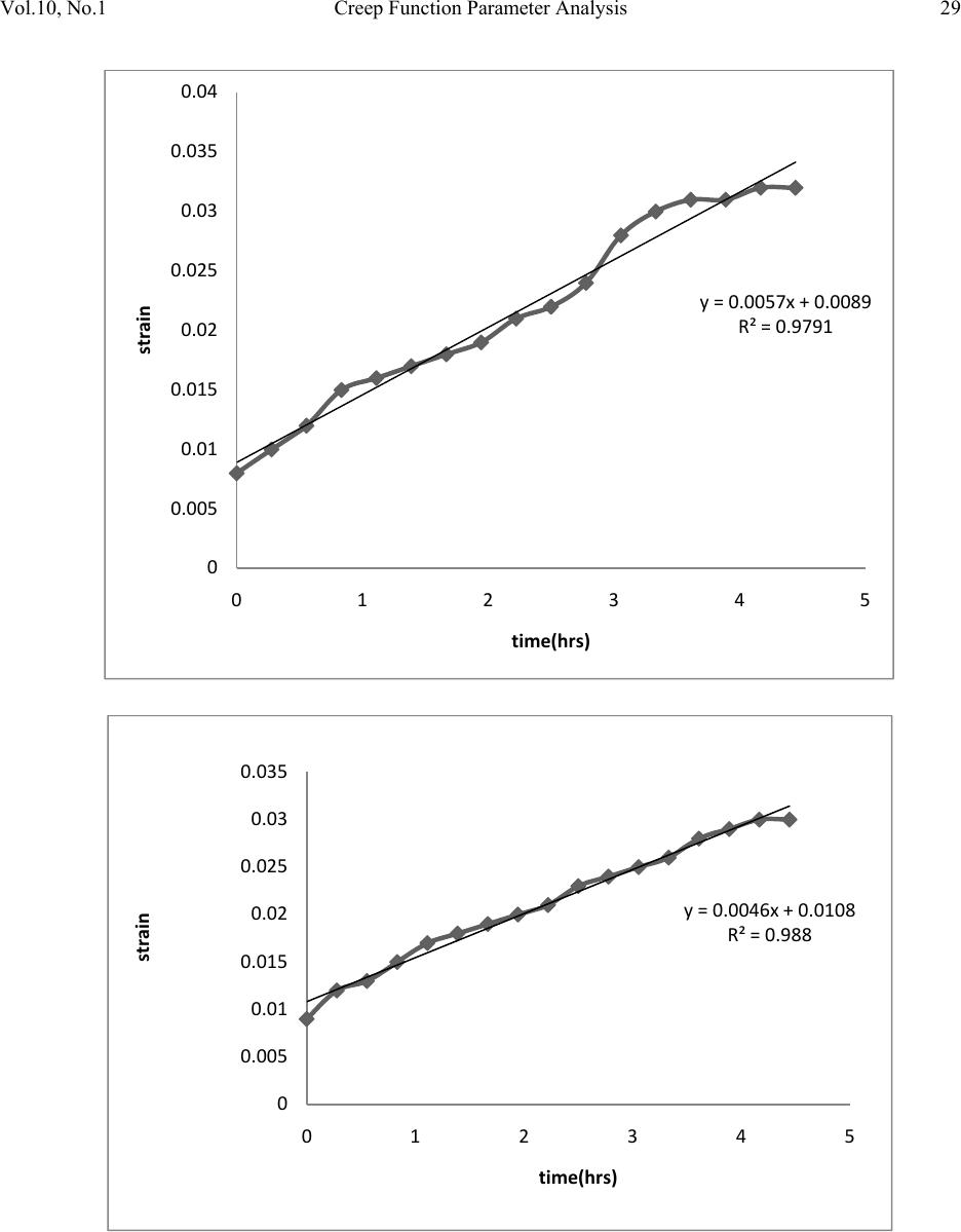 Vol.10, No.1 Creep Function Parameter Analysis 29 y=0.0057x+0.0089 R²=0.9791 0 0.005 0.01 0.015 0.02 0.025 0.03 0.035 0.04 012345 strain time(hrs) y=0.0046x+0.0108 R²=0.988 0 0.005 0.01 0.015 0.02 0.025 0.03 0.035 012345 strain time(hrs) 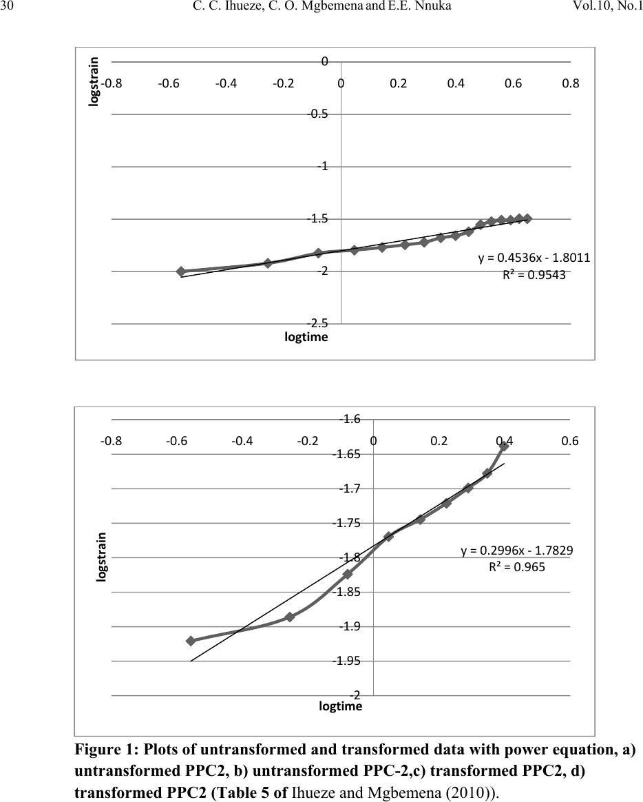 30 C. C. Ihueze, C. O. Mgbemena and E.E. Nnuka Vol.10, No.1 Figure 1: Plots of untransformed and transformed data with power equation, a) untransformed PPC2, b) untransformed PPC-2,c) transformed PPC2, d) transformed PPC2 (Table 5 of Ihueze and Mgbemena (2010)). y=0.4536x‐ 1.8011 R²=0.9543 ‐2.5 ‐2 ‐1.5 ‐1 ‐0.5 0 ‐0.8 ‐0.6 ‐0.4 ‐0.200.2 0.4 0.6 0.8 logstrain logtime y=0.2996x‐ 1.7829 R²=0.965 ‐2 ‐1.95 ‐1.9 ‐1.85 ‐1.8 ‐1.75 ‐1.7 ‐1.65 ‐1.6 ‐0.8 ‐0.6 ‐0.4 ‐0.200.2 0.4 0.6 logstrain logtime  Vol.10, No.1 Creep Function Parameter Analysis 31 2.1.1.2 For creep conditions: temperature = 50OC, static stress = 13.08MPa y=0.0054x+0.009 R²=0.9727 0 0.005 0.01 0.015 0.02 0.025 00.511.522.53 strain time y=0.0052x+0.0102 R²=0.9776 0 0.005 0.01 0.015 0.02 0.025 0 0.5 1 1.5 2 2.5 3 strain time  32 C. C. Ihueze, C. O. Mgbemena and E.E. Nnuka Vol.10, No.1 Figure 2: Plots of untransformed and transformed data with power equation, a) untransformed PPC0, b) untransformed PPC2,c) transformed PPC0, d) transformed PPC22 (Table 6 of Ihueze and Mgbemena (2010)). y=0.3546x‐ 1.8119 R²=0.9868 ‐2.5 ‐2 ‐1.5 ‐1 ‐0.5 0 ‐0.8 ‐0.6 ‐0.4 ‐0.200.2 0.4 0.6 logstrain logtime y=0.2996x‐ 1.7829 R²=0.965 ‐2 ‐1.95 ‐1.9 ‐1.85 ‐1.8 ‐1.75 ‐1.7 ‐1.65 ‐1.6 ‐0.8 ‐0.6 ‐0.4 ‐0.200.2 0.4 0.6 logstrain logtime  Vol.10, No.1 Creep Function Parameter Analysis 33 2.1.1.3 For creep conditions: temperature = 70OC, static stress = 13.08MPa y=0.099x+0.0123 R²=0.9795 0 0.01 0.02 0.03 0.04 0.05 0.06 0.07 0.08 0.09 00.2 0.4 0.6 0.8 strain time y=0.049x+0.002 R²=0.9893 0 0.005 0.01 0.015 0.02 0.025 0.03 0.035 0.04 00.2 0.4 0.6 0.8 strain time  34 C. C. Ihueze, C. O. Mgbemena and E.E. Nnuka Vol.10, No.1 Figure 3: Plots of untransformed and transformed data with power equation, a) untransformed PPC0, b) untransformed PPC2,c) transformed PPC0, d) transformed PPC2 (Table 7 of Ihueze and Mgbemena (2010)). y=0.7002x‐ 0.9953 R²=0.9821 ‐2 ‐1.8 ‐1.6 ‐1.4 ‐1.2 ‐1 ‐0.8 ‐0.6 ‐0.4 ‐0.2 0 ‐1.2 ‐1‐0.8 ‐0.6 ‐0.4 ‐0.2 0 logstrain logtime y=0.9109x‐ 1.2966 R²=0.9944 ‐2.5 ‐2 ‐1.5 ‐1 ‐0.5 0 ‐1.2 ‐1‐0.8 ‐0.6 ‐0.4 ‐0.2 0 logstrain logtime  Vol.10, No.1 Creep Function Parameter Analysis 35 2.1.2 Stress levels, creep rate and structure parameters 2.1.2.1 For stress level, 19.61MPa, temperature, 25oC y=0.0104x+0.0242 R²=0.9433 0 0.01 0.02 0.03 0.04 0.05 0.06 0.07 01234 strain time y=0.0068x+0.0244 R²=0.8594 0 0.01 0.02 0.03 0.04 0.05 0.06 01234 strain time  36 C. C. Ihueze, C. O. Mgbemena and E.E. Nnuka Vol.10, No.1 Figure 4 : Plots of untransformed and transformed data with power equation, a) untransformed PPC0, b) untransformed PPC2,c) transformed PPC0, d) transformed PPC2 (Table 8 of Ihueze and Mgbemena (2010)). y=0.2859x‐ 1.4118 R²=0.9328 ‐1.8 ‐1.6 ‐1.4 ‐1.2 ‐1 ‐0.8 ‐0.6 ‐0.4 ‐0.2 0 ‐0.8 ‐0.6 ‐0.4 ‐0.200.2 0.4 0.60.8 logstrain logtime y=0.1914x‐ 1.4594 R²=0.8804 ‐1.8 ‐1.6 ‐1.4 ‐1.2 ‐1 ‐0.8 ‐0.6 ‐0.4 ‐0.2 0 ‐0.8 ‐0.6 ‐0.4 ‐0.200.2 0.4 0.60.8 logstrain logtime  Vol.10, No.1 Creep Function Parameter Analysis 37 2.1.2.2 For stress level, 22.88MPa, temperature, 25OC y=0.0472x+0.0212 R²=0.9255 0 0.01 0.02 0.03 0.04 0.05 0.06 0.07 00.2 0.4 0.6 0.81 strain time y=0.0431x+0.0253 R²=0.7775 0 0.01 0.02 0.03 0.04 0.05 0.06 0.07 00.2 0.4 0.6 0.81 strain time  38 C. C. Ihueze, C. O. Mgbemena and E.E. Nnuka Vol.10, No.1 Figure 5: Plots of untransformed and transformed data with power equation, a) untransformed PPC0, b) untransformed PPC2,c) transformed PPC0, d) transformed PPC2 (Table 9 of Ihueze and Mgbemena (2010)) Following the graphics of this section the creep rates are evaluated as the first derivative of the linear functions of creep strain and time for different volume fractions of PPC while the creep structure parameters are evaluated with the power law model with the log transformation of the strain –time data and the results are presented in Tables 1 and 2 for various conditions. y=0.4018x‐ 1.2039 R²=0.9809 ‐1.8 ‐1.6 ‐1.4 ‐1.2 ‐1 ‐0.8 ‐0.6 ‐0.4 ‐0.2 0 ‐1.4 ‐1.2 ‐1‐0.8 ‐0.6 ‐0.4 ‐0.2 0 logstrain logtime y=0.3706x‐ 1.1868 R²=0.8802 ‐1.8 ‐1.6 ‐1.4 ‐1.2 ‐1 ‐0.8 ‐0.6 ‐0.4 ‐0.2 0 ‐1.4 ‐1.2 ‐1‐0.8 ‐0.6 ‐0.4 ‐0.2 0 logstrain logtime 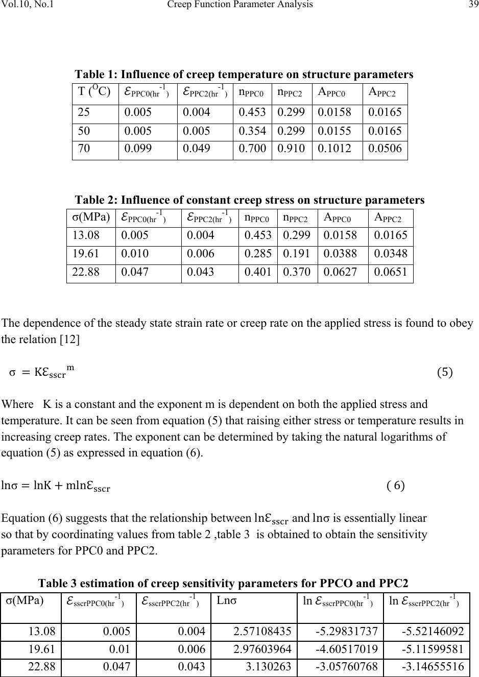 Vol.10, No.1 Creep Function Parameter Analysis 39 Table 1: Influence of creep temperature on structure parameters T (OC) PPC0(hr-1) PPC2(hr-1)nPPC0 n PPC2 A PPC0 A PPC2 25 0.005 0.004 0.4530.299 0.0158 0.0165 50 0.005 0.005 0.3540.299 0.0155 0.0165 70 0.099 0.049 0.7000.910 0.1012 0.0506 Table 2: Influence of constant creep stre s s on structure parameters σ(MPa) PPC0(hr-1) PPC2(hr-1) nPPC0 n PPC2 A PPC0 A PPC2 13.08 0.005 0.004 0.4530.299 0.0158 0.0165 19.61 0.010 0.006 0.2850.191 0.0388 0.0348 22.88 0.047 0.043 0.4010.370 0.0627 0.0651 The dependence of the steady state strain rate or creep rate on the applied stress is found to obey the relation [12] σ Where K is a constant and the exponent m is dependent on both the applied stress and temperature. It can be seen from equation (5) that raising either stress or temperature results in increasing creep rates. The exponent can be determined by taking the natural logarithms of equation (5) as expressed in equation (6). σ Equation (6) suggests that the relationship between and σ is essentially linear so that by coordinating values from table 2 ,table 3 is obtained to obtain the sensitivity parameters for PPC0 and PPC2. Table 3 estimation of creep sensitivity parameters for PPCO and PPC2 σ(MPa) sscrPPC0(hr-1) sscrPPC2(hr-1) Lnσ ln sscrPPC0(hr-1) ln sscrPPC2(hr-1) 13.08 0.005 0.0042.57108435-5.29831737 -5.52146092 19.61 0.01 0.0062.97603964-4.60517019 -5.11599581 22.88 0.047 0.0433.130263-3.05760768 -3.14655516 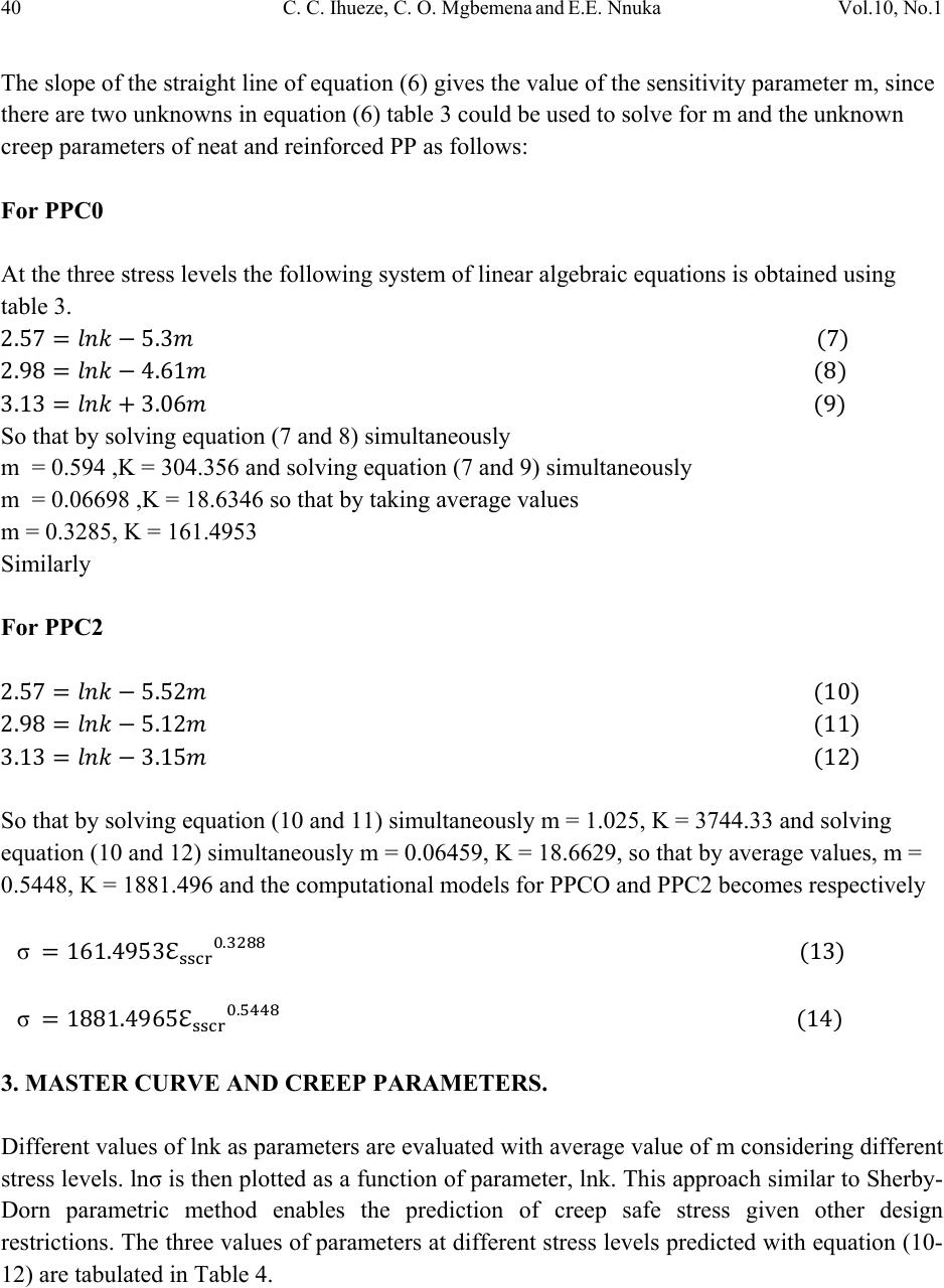 40 C. C. Ihueze, C. O. Mgbemena and E.E. Nnuka Vol.10, No.1 The slope of the straight line of equation (6) gives the value of the sensitivity parameter m, since there are two unknowns in equation (6) table 3 could be used to solve for m and the unknown creep parameters of neat and reinforced PP as follows: For PPC0 At the three stress levels the following system of linear algebraic equations is obtained using table 3. So that by solving equation (7 and 8) simultaneously m = 0.594 ,K = 304.356 and solving equation (7 and 9) simultaneously m = 0.06698 ,K = 18.6346 so that by taking average values m = 0.3285, K = 161.4953 Similarly For PPC2 So that by solving equation (10 and 11) simultaneously m = 1.025, K = 3744.33 and solving equation (10 and 12) simultaneously m = 0.06459, K = 18.6629, so that by average values, m = 0.5448, K = 1881.496 and the computational models for PPCO and PPC2 becomes respectively σ σ 3. MASTER CURVE AND CREEP PARAMETERS. Different values of lnk as parameters are evaluated with average value of m considering different stress levels. lnσ is then plotted as a function of parameter, lnk. This approach similar to Sherby- Dorn parametric method enables the prediction of creep safe stress given other design restrictions. The three values of parameters at different stress levels predicted with equation (10- 12) are tabulated in Table 4. 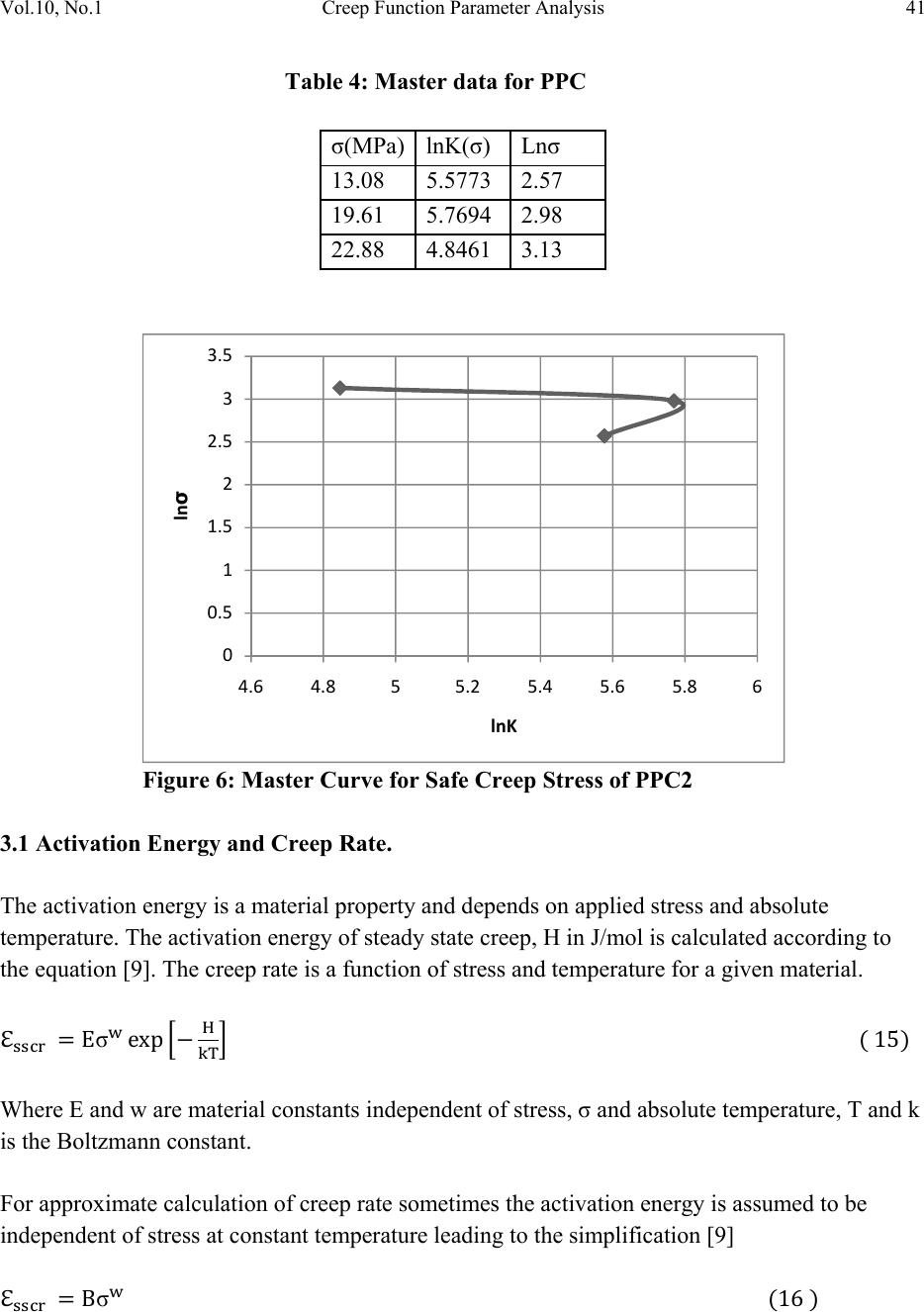 Vol.10, No.1 Creep Function Parameter Analysis 41 Table 4: Master data for PPC σ(MPa) lnK(σ) Lnσ 13.08 5.5773 2.57 19.61 5.7694 2.98 22.88 4.8461 3.13 Figure 6: Master Curve for Safe Creep Stress of PPC2 3.1 Activation Energy and Creep Rate. The activation energy is a material property and depends on applied stress and absolute temperature. The activation energy of steady state creep, H in J/mol is calculated according to the equation [9]. The creep rate is a function of stress and temperature for a given material. σ Where E and w are material constants independent of stress, σ and absolute temperature, T and k is the Boltzmann constant. For approximate calculation of creep rate sometimes the activation energy is assumed to be independent of stress at constant temperature leading to the simplification [9] σ 0 0.5 1 1.5 2 2.5 3 3.5 4.6 4.855.2 5.4 5.6 5.86 lnσ lnK 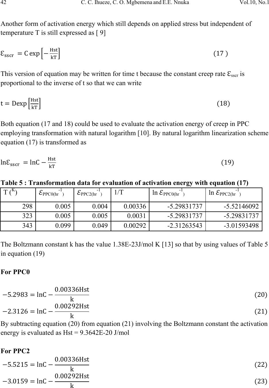 42 C. C. Ihueze, C. O. Mgbemena and E.E. Nnuka Vol.10, No.1 Another form of activation energy which still depends on applied stress but independent of temperature T is still expressed as [ 9] This version of equation may be written for time t because the constant creep rate sscr is proportional to the inverse of t so that we can write Both equation (17 and 18) could be used to evaluate the activation energy of creep in PPC employing transformation with natural logarithm [10]. By natural logarithm linearization scheme equation (17) is transformed as Table 5 : Transformation data for evaluation of activation energy with equation (17) T ( K ) PPC0(hr-1) PPC2(hr-1) 1/T ln PPC0(hr-1) ln PPC2(hr-1) 298 0.005 0.0040.00336-5.29831737-5.52146092 323 0.005 0.0050.0031-5.29831737-5.29831737 343 0.099 0.0490.00292-2.31263543-3.01593498 The Boltzmann constant k has the value 1.38E-23J/mol K [13] so that by using values of Table 5 in equation (19) For PPC0 By subtracting equation (20) from equation (21) involving the Boltzmann constant the activation energy is evaluated as Hst = 9.3642E-20 J/mol For PPC2  Vol.10, No.1 Creep Function Parameter Analysis 43 By subtracting equation (22 from equation (23) involving the Boltzmann constant the activation energy is evaluated as Hst = 7.8585E-20 J/mol. This means that the creep activation energy decreased with inclusion of nanofiller. 3.2 Master Curve by Larson-Miller Approach Approach similar to Larson-Miller is followed so that equation (18) is transformed respectively as where p is creep parameter named after Larson-Miller. This parameter is conveniently expressed as σ The parameter is expressed as a function of stress, so that by coordinating creep event time, associated temperature and stress, a plot of lnσ versus creep parameter predicts safe component stress. Table 6 data from experimental result of [10] is used to establish the master curve for predicting the PPC parameter and variables. Table 6. Creep data for parameter and variables estimation σ(MPa) T(OC) T(K) 1/T Rupture time t(hrs) Lnt f(σ) lnσ 13.08 25 298 0.00335574.41.48160454 2.57108435 13.08 50 323 0.003095982.50.91629073 2.57108435 13.08 70 343 0.002915450.7-0.35667494 2.57108435 19.61 25 298 0.00335573.61.28093385 2.97603964 22.88 25 298 0.00335570.8-0.22314355 3.13026317  44 C. C. Ihueze, C. O. Mgbemena and E.E. Nnuka Vol.10, No.1 Figure 7: lnt vs 1/T Depiction of their nonlinear relationship Figure 8 showed clearly that the creep failure model did not follow Larson-Miller parameter The creep parameters of table 5 are calculated using known Table 5 values and equation (26) for the five creep conditions but the constant lnD = D have to be evaluated first using equation (25) as Equation (27) is solved simultaneously with equations (28 and29) while equation (29) is solved simultaneously with equations (30 and31) to obtain four values of parameter, 2117.588, 7085.089 6314.9788 and 539.0835 from where the average value of parameter p is obtained as 4014.1871. ‐0.5 0 0.5 1 1.5 2 0.0028 0.00290.0030.0031 0.0032 0.0033 0.0034 0.0035 lnt 1/T  Vol.10, No.1 Creep Function Parameter Analysis 45 The value of the constant D is assumed to be same for all stress levels so that D is evaluated with equation (27) as -11.9904. With this value the parameter is evaluated at each stress level using equation (26) and table 5 as σ σ σ σ σ The above computations are presented in Table 7 for master curve for predicting creep variables Table 8: Data for Master Curve f(σ ) Lnσ 4014.18 2.57108435 4170.06 2.57108435 3989.23 2.57108435 3954.58 2.97603964 3507.58 3.13026317 Figure 8: Master curve for PPC creep conditions 0 0.5 1 1.5 2 2.5 3 3.5 3400 3600 3800 4000 4200 4400 lnσ f(σ) Lnσ Linear(Lnσ)  46 C. C. Ihueze, C. O. Mgbemena and E.E. Nnuka Vol.10, No.1 3.3 Larson-Miller Parameter and Activation Energy. The secondary stage creep activation energy can also be evaluated by expressing the parameter p as so that activation energy at various stress level can be evaluated with equation(32-36) as Hst13.08MPa = 5.5396E-20J/mol, Hst13.08MPa = 5.7547E-20J/mol, Hst13.08MPa = 5.5050E-20J/mol, Hst19.61MPa = 5.4573E-20J/mol, Hst22.08MPa = 4,845E-20J/mol, so that considering average for stress levels of 13.08MPa the activation energy becomes Hst13.08MPa = 5.7547E-20J/mol, Hst13.08MPa = 5.5998E-20J/mol, Hst19.61MPa = 5.4573E-20J/mol, Hst22.08MPa = 4,845E-20J/mol the activation energy therefore decreases with increasing stress level. 4. DISCUSSION OF RESULTS The creep curves of Figures 1a and b clearly show that the creep function strain could be perfectly represented with a linear polynomial making easy the estimation of minimum creep rate at secondary creep stage easy. A power law transformation of creep strain-time data of PPC0 and PPC2 creep data are shown in Figures 1c and d for evaluating the values of the exponent parameters nPPC0 and nPPC2 representing material constants for PPC0 and PPC2 and coefficient parameters APPC0 and APPC2 are constants which depends on stress levels. The values of the parameters evaluated show that the inclusion of nanofiller to PP has great influence on the parameters decreasing the creep rate as the constant increases with inclusion of nanofiller as found in table 1 and 2. Within the temperature range 25-50OC the parameter n is really constant with value 0.229 and the parameter A is not affected by temperature with value 0.0165. Table 2 shows that the parameter A is affected by stress level increasing with stress level and within the stress level range 13.08MPa-22.88MPa has the range 0.0165-0.061. This coefficient parameter increases the creep strain as the stress level increases. Table 3 shows that the creep rate sensitivity parameter m for PPC2 is higher as a result of incorporation of nanofiller thereby decreasing creep rate as the parameter increases. Two creep function models were used to evaluate the activation energy where it was found that PPC0 has higher activation energy with value 9.3642E-20 J/mol for the stress 13.08MPa and PPC2 has values at the stresses 13.08MPa, 19.61MPa and 22.88MPa as 5.55998E- 20J/mol,5.4573E-20J/mol and 4.845E-20J/mol respectively.  Vol.10, No.1 Creep Function Parameter Analysis 47 Two master curves were produced to aid prediction of creep safe stresses employing two versions of creep functions see Figures 6 and 7. 5. CONCLUSION This study found that 1. both the creep rate and the creep activation energy increases with applied stress and temperature and usually is lower for reinforced PP(PPC2), 2. predictions of power law coefficient and exponent of various creep functions describe, the material parameters and creep sensitivity parameters respectively thereby making way for power law creep model of PPC2 at secondary creep stage, 3. the creep response of PPC2 follows the Larson-Miller parameter which is a function of stress, 4. the activation energy is a material property and a parameter that follows Larson-Miller parameter as a function of stress and temperature and that 5. The coefficients and exponent parameters of the secondary creep stage are material constants that aid the determination of creep rate at secondary creep stage. ACKNOWLEGEMENTS. I am grateful to the authors whose materials are used. The contributions of my son, Master Chima Chukwutoo of Federal Science and Technical College, Awka, Nigeria in preparing this manuscript are appreciated. REFERENCES [1] Ritchie, R.O. “Mechanical Behaviour of materials lectures notes” University of California, Berkeley. Rhoads, 1993. [2] Eiras, D and Pessan, L.A. “Crystallization behaviour of Polypropylene/Calcium carbonate nanocomposites”.Technical paper presented on the 11th International Conference on Advanced materials at Rio de Janeiro Brazil September p.20-25,2009. [3] Hanim. H, et al. “The Effect of Calcium carbonate Nano-filler on the mechanical properties and crystallization behaviour of Polypropylene”, Malaysian Polymer Journal (MPJ), 2008, Vol 3, No. 12, p 38-49. [4] Xie X.L, Q.X. Liu, R.K.Y.Li, X.P. Zhou, Q.X. Zhang, Z. Z. Yu and Y.Mai,“Rheological and Mechanical properties of PVC/ CaCO3 Nanocomposites prepared by In-situ polymerization”, Polymer, 2004 45, p.6665-6673. [5] Di Lorenzo, M.L,Enrico.M.E,and Avell, M. “Thermal and Morphological Characterization of Poly(ethylene terepthalate)/ Calcium Carbonate Nano composites”, Journal of material service, 2002, 37, p.2351-2358.  48 C. C. Ihueze, C. O. Mgbemena and E.E. Nnuka Vol.10, No.1 [6] Chan C.M, Wu J, Li J.X, and Cheung Y.K. “Polypropylene /Calcium Carbonate Nano composites”, Polymer, 2000, 43, p.2981-2992. [7] Benham,P.P., and Warnock,F. V.,Mechanics of solids and structures ,1981, Pitman, p537-539 [8] Al-Ganainy, G.S ,Nagy, N.R,Khalifa B A and Afify R. Creep and Structure and Structure Parameters Near the Transformation Temperature of Sn-1wt% Pl Alloy, 2002, Egypt J.Sol., Vol.(25), No. (1) p57. [9] Muben, A. Machine Design, 4ed, Khanna Publishers, 2003, Delhi. p915-937. [10] Ihueze C.C. and Mgbemenna, C. Effects of Reinforcement Combinations of Calcium Carbonate Nanofiller on the Mechanical and Creep Properties of Polypropylene, 2010, JMMCE (under review). [11] Crawford, R.J. Plastics Engineering, 3rd ed, 1988, BUTTERWORTH, HEINMANN, Oxford, P46 [12] Chapara, S. C. and Canale R.P. Numerical Methods for Engineers with Programming Software Applications, 1988, McGraw-Hill, Toronto p450-453. [13] Halliday, D and Resnick, R. Fundamentals of Physics ,2ed,1981,John Wiley and Sons inc, New York,p381. |