Paper Menu >>
Journal Menu >>
 Journal of Minerals & Materials Characterization & Engineering, Vol. 9, No.10, pp.929-959, 2010 jmmce.org Printed in the USA. All rights reserved 929 Finite Elements Approaches in the Solution of Field Functions in Multidimensional Space: A Case of Boundary Value Problems Chukwutoo Christopher Ihueze*1, Okafor Emeka Christian1, Edelugo Sylvester Onyemaechi2 1Department of Industrial ⁄ Production Engineering, Nnamdi Azikiwe University Awka. 2Department of Mechanical Engineering University of Nigeria *Corresponding Author: ihuezechukwutoo @yahoo.com ABSTRACT An idealized two dimensional continuum region of GRP composite was used to develop an efficient method for solving continuum problems formulated for space domains. The continuum problem is solved by minimization of a functional formulated through a finite element procedure employing triangular elements and assumption of linear approximation polynomial. The assemblage of elements functional derivatives system of equations through FEM assembly procedure made possible the definition of a unique and parametrically defined model from which the solution of continuum configuration with an arbitrary number of scales is solved. The finite element method(FEM )developed is recommended to be applied in the evaluation of the function of functions in irregular shaped continuum whose boundary conditions are specified such as in the evaluation of displacement in structures and solid mechanics problems, evaluation of temperature distribution in heat conduction problems, evaluation of displacement potential in acoustic fluids evaluation of pressure in potential flows, evaluation of velocity in general flows, evaluation of electric potential in electrostatics, evaluation of magnetic potential in magnetostatics and in the solution of time dependent field problems. A unified computational model with standard error of 0.15 and correlation coefficient of 0.72 was developed to aid analysis and easy prediction of regional function with which the continuum function was successfully modeled and optimized through gradient search and Lagrange multipliers approach. Above all the optimization schemes of gradient search and Lagrangian multiplier confirmed local minimum of function as 0.006-0.00847 to confirm the predictions of FEM and constraint conditions. Keywords: finite element, continuum, functional of function, extremum, boundary value  930 C.C. Ihueze, O.E. Christian, E.S. Onyemaechi Vol.9, No.10 1. INTRODUCTION In calculus of variations, instead of attempting to locate points that extremize function of one or more variables that extremize quantities called functional, functions of functions that extremize the functional are found [1]. Also in the finite element process an approximate solution is sought to the problem of minimizing a functional. The concept of the finite element approach to elasticity as a process in which the total potential energy is minimized with respect to nodal displacements can obviously be extended to a variety of physical problems in which an extremum principle exists. The two concepts are combined in this study. Zienkiewicz and Cheung [2] applied similar approach to solve continuum problem expressed in derivative format employing the concept of functional minimization with FEM. Above all, there are many problems encountered in engineering and physics where the minimization of the integrated quantity usually referred as functional and subject to some boundary conditions results in the exact solution.This functional may represent a physical recognizable variable in some instances, for many purposes it is simply a mathematically defined entity. The geometry of field quantities or continuum may be a problem to close form solution of field functions encountered in engineering and science that appropriate algorithm becomes necessary to obtain optimum solution, it is then necessary to employ calculus of variation principles and FEM to obtain optimum continuum field functions whose boundary conditions are specified. The engineering field continuum problems can be basically in form of wave phenomenon, diffusion phenomenon and potential phenomenon usually represented by hyperbolic, parabolic and elliptic differential equations respectively [3]. The objective of this study is therefore to present a methodical approach to solve multiple dimensional field problems using integrated variational and FEM approach to establish relations for all elements functional of continuum where the minimization of the elements functionals system and solution are expected to give the stationary values of the function which extremize the functional. 2. THEORETICAL BACKGROUND A finite element model of a two dimensional quadratic function is expected to present a methodical approach to employ for solution of multidimensional field functions that may have regular or irregular field regions. Zienkiewicz and Cheung [2] presented Euler theorem to approximate field functions if the integral or functional of the form . I (u) = ∫∫∫ f( x,y,z,u, ∂u ∂x , ∂u ∂y , ∂u ∂z ) dxdydz (1)  Vol.9, No.10 Finite Elements Approaches in the Solution of Field Functions 931 is to be minimized. The necessary and sufficient condition for this minimum to be reached is that the unknown function u (x, y, z) should satisfy the following differential equation ∂ ∂x [∂f ∂(∂u/∂x) ] + ∂ ∂y [∂f ∂(∂u/∂y) ] + ∂ ∂z [∂f ∂(∂u/∂z) ] - ∂f ∂u = 0 (2) within the same region, provided u satisfies the same boundary conditions in both cases,while the equation governing the behaviour of unknown physical quantity u can generally be expressed as ∂ ∂x (kx ∂u ∂x ) + ∂ ∂y (ky ∂u ∂y ) + ∂ ∂z ( kz ∂u ∂z ) + Q = 0 (3) where u = unknown function assumed to be single valued within the region kx, ky, kz , Q = specified functions of x, y, z x, y, z = space variables The equivalent formulation to that of equation (3) is the requirement that the volume integral given below and taken over the whole region, should be χ =∫∫∫ {1 2 [kx (∂u ∂x ) 2 + ky(∂u ∂y )2 + kz(∂u ∂z )2] - Q u}dxdydz (4) subject to u obeying the same boundary conditions. For two dimensional differential equation representing some physical quantities then χ =∫∫ {1 2 [kx (∂u ∂x ) 2 + ky(∂u ∂y )2] - Q u}dxdy (5) For the case of our interest, the equivalent functional to be minimized for 2-D Laplace model reduces to χ =∫∫ {1 2 [kx (∂u ∂x ) 2 + ky(∂u ∂y )2] }dxdy (6) The finite element version of an integrated functional is obtained and minimized with respect to degrees of freedoms of the associated elements. The element functional equations are assembled and boundary conditions applied, resulting in a system of equations equal to the number of unconstrained degrees of freedoms of the continuum. 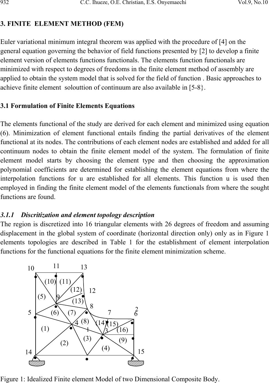 932 C.C. Ihueze, O.E. Christian, E.S. Onyemaechi Vol.9, No.10 3. FINITE ELEMENT METHOD (FEM) Euler variational minimum integral theorem was applied with the procedure of [4] on the general equation governing the behavior of field functions presented by [2] to develop a finite element version of elements functions functionals. The elements function functionals are minimized with respect to degrees of freedoms in the finite element method of assembly are applied to obtain the system model that is solved for the field of function . Basic approaches to achieve finite element solouttion of continuum are also available in [5-8}. 3.1 Formulation of Finite Elements Equations The elements functional of the study are derived for each element and minimized using equation (6). Minimization of element functional entails finding the partial derivatives of the element functional at its nodes. The contributions of each element nodes are established and added for all continuum nodes to obtain the finite element model of the system. The formulation of finite element model starts by choosing the element type and then choosing the approximation polynomial coefficients are determined for establishing the element equations from where the interpolation functions for u are established for all elements. This function u is used then employed in finding the finite element model of the elements functionals from where the sought functions are found. 3.1.1 Discritization and element topology description The region is discretized into 16 triangular elements with 26 degrees of freedom and assuming displacement in the global system of coordinate (horizontal direction only) only as in Figure 1 elements topologies are described in Table 1 for the establishment of element interpolation functions for the functional equations for the finite element minimization scheme. Figure 1: Idealized Finite element Model of two Dimensional Composite Body. . . . . . . . . . . . . . . . (1) (2) (3) (4) (9) (6) (7) (8) (14)(15) (16) (13) (12) (11) (10) (5) 10 11 13 5 14 15 3 6 7 8 12 4 9 1 2  Vol.9, No.10 Finite Elements Approaches in the Solution of Field Functions 933 Table 1: Element Topology Description. Element Number Active degrees of freedom of elements Element coordinates Element nodes 1 u5, u4, u14, v5, v4, v14 (0,0), (0,21), (16,16) 14, 5, 4 2 u1, u4, u14, v1, v4, v14 (0,0), (16,16), (21, 0) 14, 4, 1 3 u1, u4, u3, v1, v4, v3 (21, 0), (16, 16), (25, 10) 1, 4, 3 4 u1, u3, u15, v1, v3, v15 (21, 0), (21, 0), (25, 10) 1, 3, 15 5 u5, u10, u9, v5, v10, v9 (0, 21), (0, 37), (10, 25) 5, 10, 9 6 u5, u9, u4, v5, v9, v4 (0, 21), (0, 25), (16, 16) 5, 9, 4 7 u9, u4, u8, v9, v4, v8 (16, 16), (10, 25), (22, 13)4, 9, 8 8 u8, u4, u3, v8, v4, v3 (16, 16), (22, 23), (25, 10)4, 8, 3 9 u15, u3, u2, v15, v3, v2 (25, 10), (35, 10), (35, 0) 15, 3, 2 10 u9, u10, u11, v9, v10, v11 (0, 37), (10, 37), (10, 25) 9, 10, 11 11 u9, u11, u13, v9, v11, v13 (10, 25), (10, 37), (18, 37)9, 11, 13 12 u9, u13, u12, v9, v13, v12 (10, 25), (18, 37), (19, 29)9, 13, 12 13 u9, u12, u8, v9, v12, v8 (10, 25), (19, 29), (22, 23)9, 12, 8 14 u3, u8, u7, v3, v8, v7 (25, 10), (22, 23), (29, 19)3, 8, 7 15 u3, u7, u6, v3, v7, v6 (25, 11), (29, 19), (35, 18)3, 7, 6 16 u3, u6, u12, v3, v6, v12 (25, 10), (35, 18), (35, 10)3, 6, 2 3.2 Determination of FEM Characteristics 3.2.1 Element 1 interpolation and functional equation formulation By assuming a linear approximation polynomial of the form yaxaayxu 210 ),( (1) and following the method of Ihueze etal (2009) and Asterly (1992) 5[0, 21] 4[16, 16] 14[0, 0] 1 u v u4 v5 1 5 v14 u14 v4 u5 4 14  934 C.C. Ihueze, O.E. Christian, E.S. Onyemaechi Vol.9, No.10 Where a0, a1, a2 are called polynomial coefficients or shape constants so that by passing (1) through the nodes of element1the system of unknown function of the element becomes: 142141014 yaxaau 424104yaxaau 525105 yaxaau Putting the above polynomial function in matrix form then 5 4 14 2 1 0 55 44 1414 1 1 1 u u u a a a yx yx yx By applying Crammers rule 14441455141454455414 2 1 0yxyxuyxyxuyxyxua A (2) 414514545414 2 1 1yyuyyuyyuaA 144551444514 2 1 2xxuxxuxxua A Substituting (2) in (1) then yaxaau 2101 yxxuxxuxxu xyyuyyuyyu yxyxuyxyxuyxyxuu A A A 144551444514 2 1 414514545414 2 1 14441455141454455414 2 1 1 (3) Recall that the approximation function is given as 55441414 uNuNuNu (4) Comparing (5) and (6) we evaluate shape and interpolation function thus  Vol.9, No.10 Finite Elements Approaches in the Solution of Field Functions 935 yxxxyyyxyxyxN A45544554 2 1 14 , (5) yxxxyyyxyxyxN A514145514145 2 1 4, yxxxyyyxyxyxN A144414144414 2 1 5, But A = 1444145141454554 2 1yxyxyxyxyxyx = 168mm2 (6) where A= area of triangular element so that yxN 165336 336 1 14 xN 21 336 1 4 yxN 1616 336 1 5 Substituting (7) in (4) 5 336 1 4 336 1 14 336 1161621165336 uyxuxuyxu 336 16 336 21 336 5 5 414 u uu x u 336 16 336 16 5 14 u u y u By assuming a two dimensional Laplace function for the continuum function of the form ∂2u ∂x2 + ∂2u ∂y2 = 0 (10) The minimum function integral called functional to be minimized becomes in which case kx = ky = kz = 1 and Q = 0 (11) So that (4 ) reduces to dxdyx y u x u22 2 1 (9) (8) (12) (7)  936 C.C. Ihueze, O.E. Christian, E.S. Onyemaechi Vol.9, No.10 By substitutingg the first partial derivatives of the element 4 interpolation functions in ( 12) with dxdy = A = 168 2 5 2 454145144 2 14 762.0656.0_524.0313.0418.0 uuuuuuuuux (13) By differentiating w.r.t.u14,u4,and u5 5.0*524.0313.0836.0 5414 14 uuu u x 5.0*313.0312.1 5144 4 uuu u x 5.0*524.0524.1 4145 5 uuu u x 3.2.2 Element 2 interpolation and functional equation formulation By assuming a linear approximation polynomial of the form yaxaayxu 210, )( (15) Passing (15) through the nodes then 142141014 yaxaau 121101 yaxaau 424104 yaxaau Putting the system in matrix form then 4 1 14 2 1 0 44 11 1414 1 1 1 u u u a a a yx yx yx (14) u u1 v4 v [16, 16] [21, 0] [0, 0] 2 4 14 2 4 u14 v14 v1 u4 1 14  Vol.9, No.10 Finite Elements Approaches in the Solution of Field Functions 937 By applying Crammers rule, 14144114144114 2 1 0xxuyyuyxyxua A 414114414141441 2 1 1xxuyyuyxyxuaA 14141441411144 2 1 2xxuyyuyxyxua A (16) Substituting (16) in (15) 14144114144114 2 1xxuyyuyxyxuu A 414114414141441 xxuyyuyxyxu (17) 141411441411144 xxuyyuyxyxu Recalling that the approximation function is 44111414 uNuNuNu (18) Comparing (18) and (17) then yxxxyyyxyxNA14411441 2 1 14 yxxxyyyxyxN A414144414144 2 1 1 yxxxyyyxyxN A141114141114 2 1 4 (19) But A = 1411144141441441 2 1yxyxyxyxyxyx =168mm2 (20) so that yxxN 5163362116160336 336 1 336 1 14 yxyxN 16161600160 336 1 336 1 1 yyN 2102100336 1 336 1 4 (21) Substituting (22) into (18) 4 336 1 1 336 1 14 336 1211616516336uyuyuyxu (22) 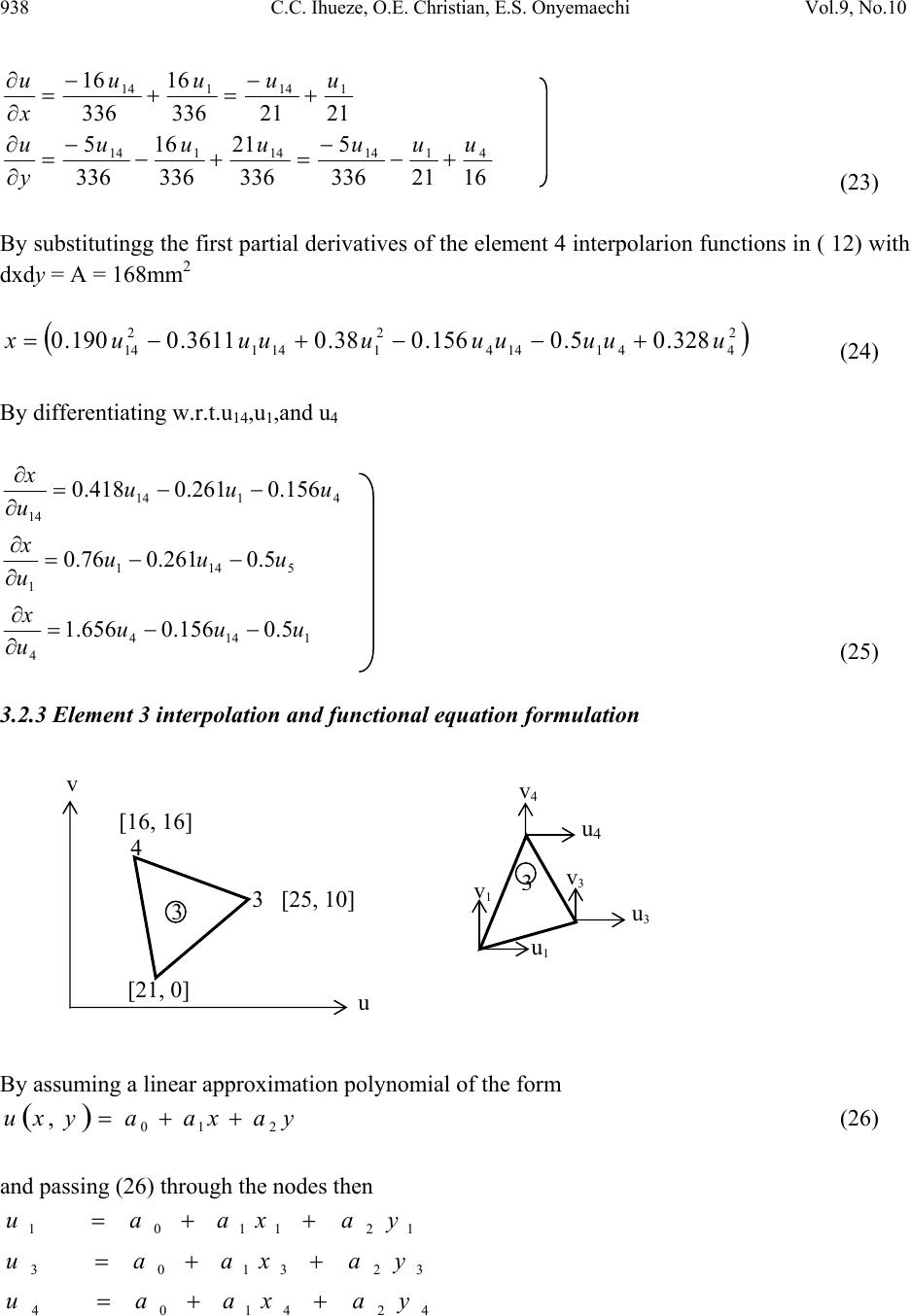 938 C.C. Ihueze, O.E. Christian, E.S. Onyemaechi Vol.9, No.10 2121336 16 336 16 114114 uuuu x u 1621336 5 336 21 336 16 336 5411414114 uuuuuu y u (23) By substitutingg the first partial derivatives of the element 4 interpolarion functions in ( 12) with dxdy = A = 168mm2 2 441144 2 1141 2 14 328.05.0156.038.03611.0190.0 uuuuuuuuux (24) By differentiating w.r.t.u14,u1,and u4 4114 14 156.0261.0418.0 uuu u x 5141 1 5.0261.076.0 uuu u x 1144 4 5.0156.0656.1 uuu u x (25) 3.2.3 Element 3 interpolation and functional equation formulation By assuming a linear approximation polynomial of the form yaxaayxu 210 , (26) and passing (26) through the nodes then 121101 yaxaau 323103 yaxaau 424104 yaxaau v [16, 16] 4 3 [25, 10] [21, 0] 3 u v1 u1 u3 v3 v4 u4 3 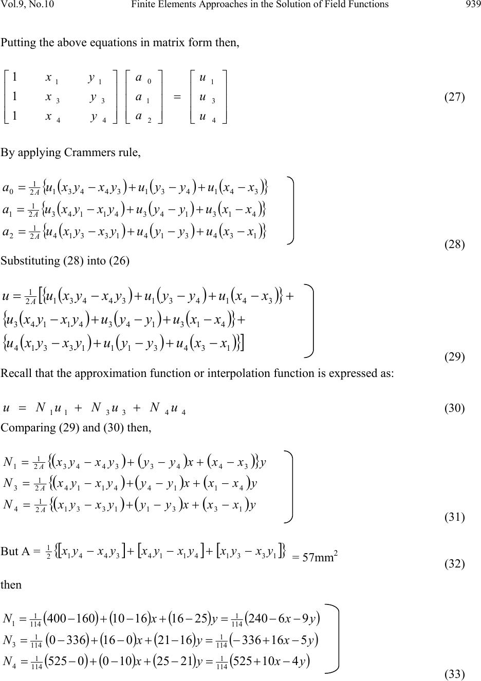 Vol.9, No.10 Finite Elements Approaches in the Solution of Field Functions 939 Putting the above equations in matrix form then, 4 3 1 2 1 0 44 33 11 1 1 1 u u u a a a yx yx yx (27) By applying Crammers rule, 34143134431 2 1 0xxuyyuyxyxua A 41314341143 2 1 1xxuyyuyxyxua A 13431413314 2 1 2xxuyyuyxyxua A (28) Substituting (28) into (26) 34143134431 2 1xxuyyuyxyxuu A 41314341143 xxuyyuyxyxu 13431113314 xxuyyuyxyxu (29) Recall that the approximation function or interpolation function is expressed as: 443311 uNuNuNu (30) Comparing (29) and (30) then, yxxxyyyxyxN A34433443 2 1 1 yxxxyyyxyxN A41144114 2 1 3 yxxxyyyxyxNA13311331 2 1 4 (31) But A = 133141143441 2 1yxyxyxyxyxyx = 57mm2 (32) then yxyxN 9624025161610160400 114 1 114 1 1 yxyxN 51633616210163360114 1 114 1 3 yxyxN 41052521251000525 114 1 114 1 4 (33) 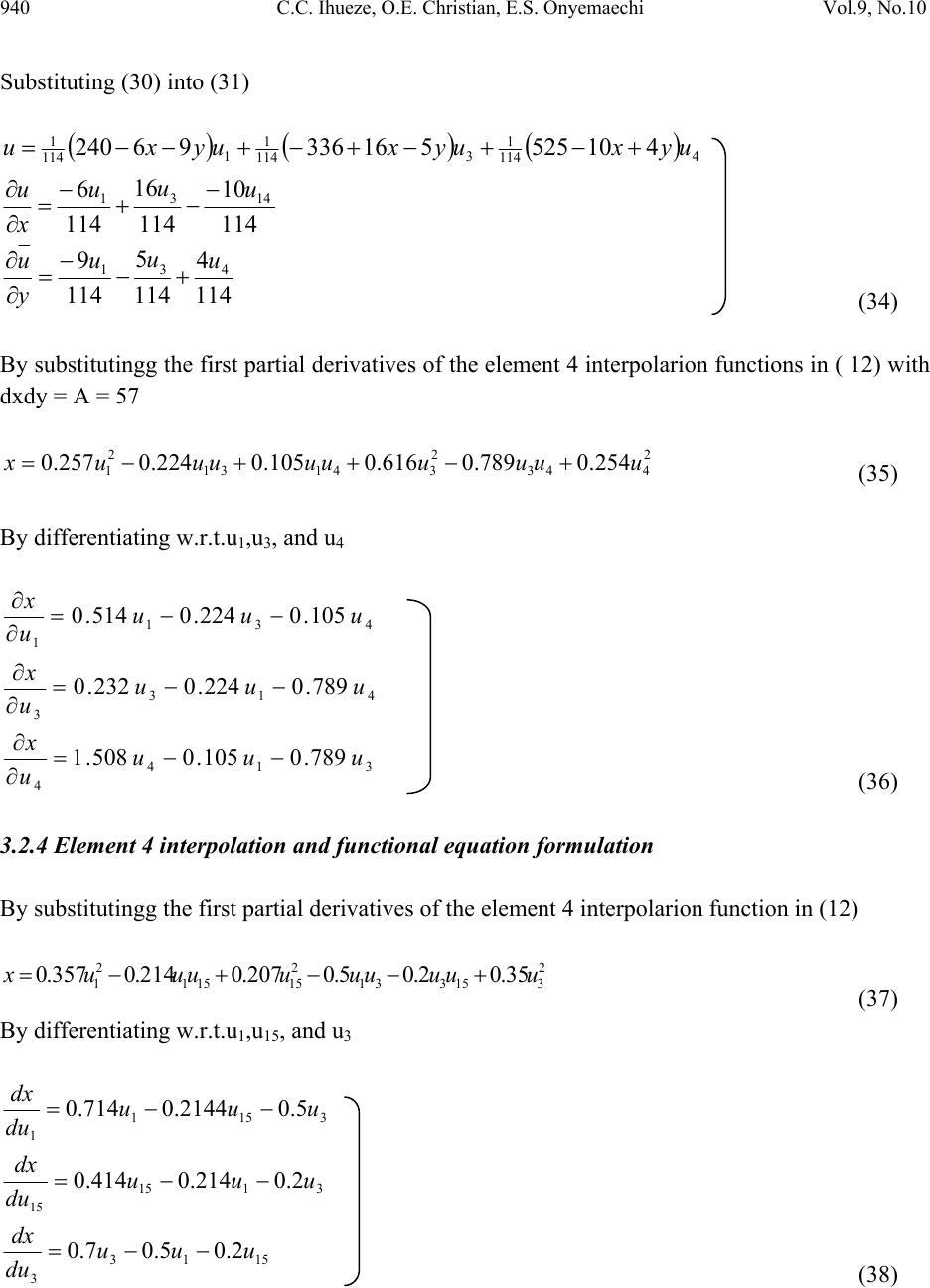 940 C.C. Ihueze, O.E. Christian, E.S. Onyemaechi Vol.9, No.10 Substituting (30) into (31) 4 114 1 3 114 1 1 114 141052551633696240 uyxuyxuyxu 114 10 114 16 114 614 3 1u u u x u 114 4 114 5 114 94 3 1u u u y u (34) By substitutingg the first partial derivatives of the element 4 interpolarion functions in ( 12) with dxdy = A = 57 2 443 2 34131 2 1254.0789.0616.0105.0224.0257.0 uuuuuuuuux (35) By differentiating w.r.t.u1,u3, and u4 431 1 105.0224.0514.0 uuu u x 413 3 789.0224.0232.0 uuu u x 314 4 789.0105.0508.1uuu u x (36) 3.2.4 Element 4 interpolation and functional equation formulation By substitutingg the first partial derivatives of the element 4 interpolarion function in (12) 2 315331 2 15151 2 135.02.05.0207.0214.0357.0 uuuuuuuuux (37) By differentiating w.r.t.u1,u15, and u3 3151 1 5.02144.0714.0 uuu du dx 3115 15 2.0214.0414.0 uuu du dx 1513 3 2.05.07.0 uuu du dx (38) 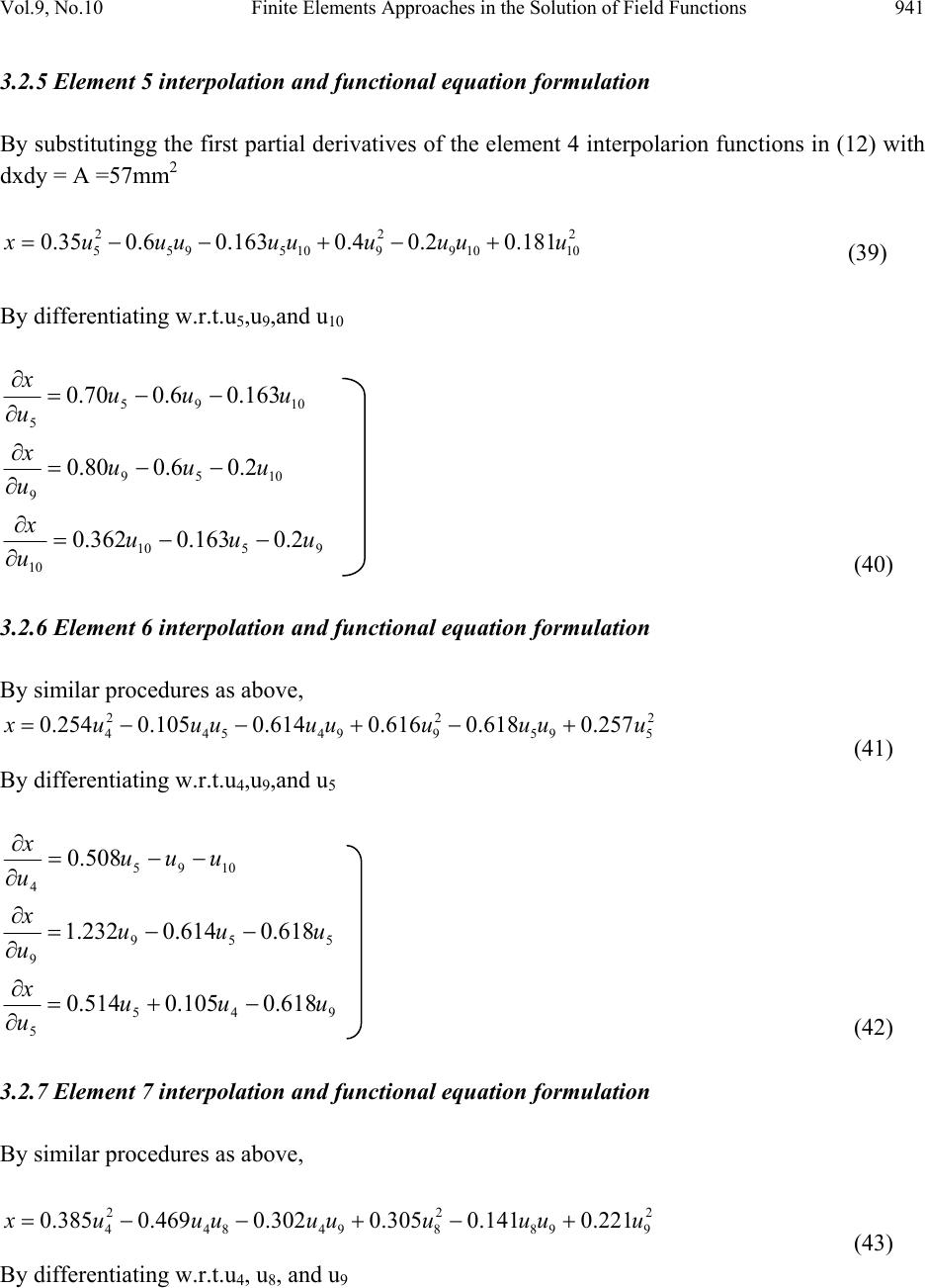 Vol.9, No.10 Finite Elements Approaches in the Solution of Field Functions 941 3.2.5 Element 5 interpolation and functional equation formulation By substitutingg the first partial derivatives of the element 4 interpolarion functions in (12) with dxdy = A =57mm2 2 10109 2 910595 2 5181.02.04.0163.06.035.0 uuuuuuuuux (39) By differentiating w.r.t.u5,u9,and u10 1095 5 163.06.070.0 uuu u x 1059 9 2.06.080.0 uuu u x 9510 10 2.0163.0362.0 uuu u x (40) 3.2.6 Element 6 interpolation and functional equation formulation By similar procedures as above, 2 595 2 99454 2 4257.0618.0616.0614.0105.0254.0 uuuuuuuuux (41) By differentiating w.r.t.u4,u9,and u5 1095 4 508.0 uuu u x 559 9 618.0614.0232.1 uuu u x 945 5 618.0105.0514.0 uuu u x (42) 3.2.7 Element 7 interpolation and functional equation formulation By similar procedures as above, 2 998 2 89484 2 4221.0141.0305.0302.0469.0385.0 uuuuuuuuux (43) By differentiating w.r.t.u4, u8, and u9  942 C.C. Ihueze, O.E. Christian, E.S. Onyemaechi Vol.9, No.10 984 4 302.0469.077.0 uuu u x 948 8 141.0469.061.1 uuu u x 949 9 141.0302.0442.0 uuu u x (44) 3.2.8 Element 8 interpolation and functional equation formulation By similar procedures as above, 2 484 2 84383 2 3450.0530.0295.0369.061.0215.0 uuuuuuuuux (45) By differentiating w.r.t.u3,u8,and u4 483 3 369.0061.0430.0 uuu u x 438 8 530.0061.0590.0 uuu u x 934 4 530.0369.090.0 uuu u x (46) 3.2.9 Element 9 interpolation and functional equation formulation By similar procedures as above, 152 2 15 2 332 2 25.025.025.05.05.0 uuuuuuux (47) By differentiating w.r.t.u2,u3,and u15 1532 2 5.05.0 uuu u x 23 3 5.05.0 uu u x 215 15 5.05.0 uu u x (48) 3.2.10 Element 10 interpolation and functional equation formulation By similar procedures as above,  Vol.9, No.10 Finite Elements Approaches in the Solution of Field Functions 943 119 2 9 2 101110 2 11 417.0208.03.061.0508.0 uuuuuuux (49) By differentiating w.r.t.u11,u10, and u9 91011 11 417.06.0016.1 uuu u x 1110 10 6.06.0 uu u x 119 9 417.0416.0 uu u x (50) 3.2.11 Element 11 interpolation and functional equation formulation By similar procedures as above, 119 2 9 2 111311 2 13 333.0167.0542.075.0375.0 uuuuuuux (51) By differentiating w.r.t.u9,u13, and u1 119 9 333.0334.0 uu u x 1113 13 75.075.0 uu u x 91311 11 333.075.0084.1 uuu u x (52) 3.2.12 Element 12 interpolation and functional equation formulation By similar procedures as above, 2 131312 2 12139129 2 9319.0158.068.0151.068.0214.0 uuuuuuuuux By differentiating w.r.t.u9,u12, and u13 13129 9 151.0684.0428.0 uuu u x 3912 12 158.0684.0368.1 uuu u x 12913 13 158.0151.0638.0 uuu u x (53)  944 C.C. Ihueze, O.E. Christian, E.S. Onyemaechi Vol.9, No.10 3.2.13 Element 13 interpolation and functional equation formulation By similar procedures as above, 2 9129 2 1298128 2 8170.0182.0561.0386.0758.0367.0 uuuuuuuuux (54) By differentiating w.r.t.u8, u12, and u9 9128 8 386.0758.0734.0 uuu u x 9812 12 182.0758.0122.1 uuu u x 1289 9 182.0386.034.0 uuu u x (55) 3.2.14 Element 14 interpolation and functional equation formulation By similar procedures as above, 2 887 2 78373 2 3307.0665.0563.0051.0462.0206.0 uuuuuuuuux (56) By differentiating w.r.t.u3,u7, and u8 873 3 051.0462.0412.0 uuu u x 837 7 665.0462.0126.1 uuu u x 738 8 665.051.0614.0 uuu u x (57) 3.2.15 Element 15 interpolation and functional equation formulation By similar procedures as above, 2 776 2 67363 2 3716.0923.0385.051.0154.0178.0 uuuuuuuuux By differentiating w.r.t.u3, u6, and u7  Vol.9, No.10 Finite Elements Approaches in the Solution of Field Functions 945 763 3 51.0154.0356.0 uuu u x 763 3 51.0154.0356.0 uuu u x 637 7 923.051.0432.1 uuu u x (58) 3.2.16 Element 16 interpolation and functional equation formulation By similar procedures as above, 2 662 2 232 2 3313.0625.0513.04.02.0 uuuuuuux By differentiating w.r.t.u3, u2 and u6 23 3 4.04.0 uu u x 632 2 625.04.0026.0 uuu u x 26 6 625.0626.0 uu u x (59) 4. SYSTEM ELEMENTS ASSEMBLY ALGORITHMS The algorithms for element assembly involves the addition of all elements contributing to minimization dXe du , this leads to system of equations that equals the degrees of freedoms in the continuum, the derivatives are then added in a special format called assembly. There are 15 effective degrees of freedoms for the assembly of 16 elements dXe ui = 0, i = 1, 2, 3,……, 16 For i = 1, Xe u1 = 0 (60) i = 2, Xe u2 = 0 (61)  946 C.C. Ihueze, O.E. Christian, E.S. Onyemaechi Vol.9, No.10 i = 3, Xe u3 = 0 (62) i = 4, Xe u4 = 0 (63) i = 5, Xe u5 = 0 (64) i = 6, Xe u6 = 0 (65) i = 7, Xe u7 = 0 (66) i = 8, Xe u8 = 0 (67) i = 9, Xe u9 = 0 (68) i = 10, Xe u10 = 0 (69) i = 11, Xe u11 = 0 (70) i = 12, Xe u12 = 0 (71) i = 13, Xe u13 = 0 (72) i = 14, Xe u14 = 0 (73) i = 15, Xe u15 = 0 (74) 5. ELEMENTS EQUATIONS ASSEMBLY All the partial derivatives resulting from the minimization scheme with respect to the fifteen (15) active degrees of freedom (DOF) are added as follows the superscripts on these equations denote element sources: X u1 = Xe u1 = 0 = X2 u1 + X3 u1 + X4 u1 = 1.988u1 – 0.724u3 - 0.105u4 – 0.5u5 – 0.261u14 – 0.214u15 (75) X u2 = Xe u2 = 0 = X9 u2 + X16 u2 = 1.026u2 – 0.9u3 – 0.625u6 - 0.5u15 (76)  Vol.9, No.10 Finite Elements Approaches in the Solution of Field Functions 947 X u3 = Xe u3 = 0 = X16 u3 + X15 u3 + X14 u3 + X9 u3 + X4 u3 + X3 u3 + X8 u3 = - 0.724u1 – 0.9u2 + 3.03u3 – 1.158u4 + 0.154u6 – 0.972u7 – 0.001u8 - 0.2u15 (77) X u4 = Xe u4 = 0 = X1 u4 + X2 u4 + X3 u4 + X6 u4 + X7 u4 + X8 u4 = -1.158u3 + 5.49u4 – 0.395u1 + 0.008u5 – 0.469u8 – 1.832u9 – u10 – 0.001u14 (78) X u5 = Xe u5 = 0 = X1 u5 + X5 u5 + X6 u5 = - 0.409u4 + 1.979u5 – 1.218u9 – 0.163u10 – 0.262u14 (79) X u6 = Xe u6 = 0 = X15 u6 + X16 u6 = 1.396u6 – 0.625u2 + 0.154u3 – 0.923u7 (80) X u7 = Xe u7 = 0 = X15 u7 + X14 u7 = 2.549u7 – 0.972u3 – 0.923u6 – 0.665u9 (81) X u8 = Xe u8 = 0 = X7 u8 + X8 u8 + X13 u8 + X14 u8 = 0.449u3 – 0.999u4 – 0.665u7 + 3.548u8 + 0.245u9 – 0.758u12 (82) X u9 = Xe u9 = 0 = X13 u9 + X12 u9 + X11 u9 + X10 u9 + X7 u9 + X6 u9 + X5 u9 = - 0.302u4 – 1.832u5 + 0.386u8 + 3.851u9 – 0.20u10 – 0.75u11 + 0.502u12 + 0.151u13 (83) X u10 = Xe u10 = 0 = X5 u10 + X10 u10 = - 0.163u5 – 0.2u9 + 0.962u10 – 0.6u11 (84) X u11 = Xe u11 = 0 = X11 u11 + X10 u11 = - 0.75u9 – 0.6u10 + 2.1u11 - 0.75u13 (85) X u12 = Xe u12 = 0 = X13 u12 + X12 u12 = - 0.158u13 + 0.758u8 + 0.502u9 + 2.49u12 (86)  948 C.C. Ihueze, O.E. Christian, E.S. Onyemaechi Vol.9, No.10 X u13 = Xe u13 = 0 = X11 u13 + X12 u13 = - 0.151u9 – 0.75u11 – 0.158u12 + 1.388u13 (87) X u14 = Xe u14 = 0 = X2 u14 + X1 u14 = - 0.261u1 – 0.313u4 – 0.262u5 + 0.836u14 (88) X u15 = Xe u15 = 0 = X4 u15 + X9 u15 = - 0.214u1 – 0.5u2 – 0.2u3 + 0.914u15 (89) 6. APPLICATION OF BOUNDARY CONDITION In this work a special case where displacements at the boundaries are limited to 0.5mm for an irregular continuum is considered to predict continuum displacement, strain and stress functions, while the constrained conditions are taken as zero so that by equating u14 = u15 = 0 and u2 = u5= u6 = u8 = u10= u13 = 0.50 , (75 - 89) transform to the following: 1.988u1 – 0.724u3 – 0.105u4 = 0.25 (90) 0.900u3 = 0.201 (91) - 0.724u1 + 3.03u3 – 0.158u4 – 0.972u7 = 0.374 (92) - 1.158u3 + 5.490u4 – 0.395u1 = 0.731 (93) - 0.409u4 – 1.218u9 = - 0.907 (94) 0.154u3 – 0.923u7 = - 0.386 (95) 2.549u7 – 0.972u3 – 0.665u9 = 0.462 (96) 0.449u3 – 0.999u4 – 0.665u7 + 0.245u9 – 0.758u12 = - 1.774 (97) 3.851u9 – 0.302u4 – 0.75u11 + 0.502u12 = 0.748 (98) - 0.200u9 – 0.600u11 = - 0.400 (99)  Vol.9, No.10 Finite Elements Approaches in the Solution of Field Functions 949 2.100u11 – 0.750u9 = 0.675 (100) - 0.153u3 + 0.502u9 + 2.490u12 = - 0.379 (101) - 0.151u9 – 0.750u11 – 0.158u12 = - 0.694 (102) - 0.261u1 – 0.313u4 = 0.131 (103) - 0.214u1 – 0.200u3 = 0.250 (104) 7. SOLUTION AND POST PROCESSING FOR CONTINUUM FUNCTION The following nodal displacements in mm are further evaluated by first evaluating u3 = 0.222 from (91) so that other nodal values of the displacement function is as presented in Table 2. The first partial derivatives of the interpolation function evaluated with active degree of freedom in of element with respect to the x axis gives the slope of the function and also gives the value of the strain as presented in Table 2. The computations are achieved with sixteen elements interpolation functions associated with the elements global coordinate axis. The strains so computed may be used with Hooke’s law of elasticity to predict the stress distribution function at the respective nodes when the elastic modulus is known from literature. Table 2: FEM Results. n(nodes) u(displacement) (strain) 1 0.210 0.02 2 0.500 0.01 3 0.222 0.02 4 0.059 0.015 5 0.500 0.023 6 0.500 0.015 7 0.455 0.082 8 0.500 0.054 9 0.725 0.028 10 0.500 0.01 11 0.424 0.116 12 0.500 0 13 0.500 0.167 14 0.000 0.026 15 0.000 0.011 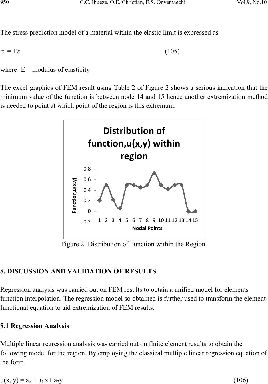 950 C.C. Ihueze, O.E. Christian, E.S. Onyemaechi Vol.9, No.10 The stress prediction model of a material within the elastic limit is expressed as σ = Е (105) where Е = modulus of elasticity The excel graphics of FEM result using Table 2 of Figure 2 shows a serious indication that the minimum value of the function is between node 14 and 15 hence another extremization method is needed to point at which point of the region is this extremum. Figure 2: Distribution of Function within the Region. 8. DISCUSSION AND VALIDATIO N OF RESULTS Regression analysis was carried out on FEM results to obtain a unified model for elements function interpolation. The regression model so obtained is further used to transform the element functional equation to aid extremization of FEM results. 8.1 Regression Analysis Multiple linear regression analysis was carried out on finite element results to obtain the following model for the region. By employing the classical multiple linear regression equation of the form u(x, y) = ao + a1 x+ a2y (106) ‐0.2 0 0.2 0.4 0.6 0.8 1 2 3 4 5 6 7 8 9101112131415 Function,u(x,y) NodalPoints Distributionof function,u(x,y)within reg i on 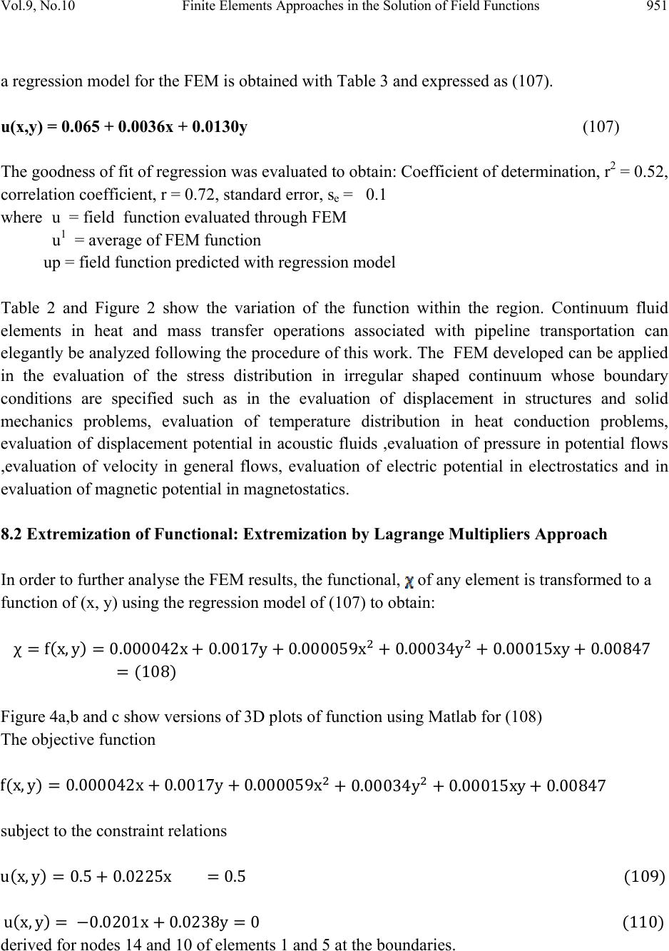 Vol.9, No.10 Finite Elements Approaches in the Solution of Field Functions 951 a regression model for the FEM is obtained with Table 3 and expressed as (107). u(x,y) = 0.065 + 0.0036x + 0.0130y (107) The goodness of fit of regression was evaluated to obtain: Coefficient of determination, r2 = 0.52, correlation coefficient, r = 0.72, standard error, se = 0.1 where u = field function evaluated through FEM u1 = average of FEM function up = field function predicted with regression model Table 2 and Figure 2 show the variation of the function within the region. Continuum fluid elements in heat and mass transfer operations associated with pipeline transportation can elegantly be analyzed following the procedure of this work. The FEM developed can be applied in the evaluation of the stress distribution in irregular shaped continuum whose boundary conditions are specified such as in the evaluation of displacement in structures and solid mechanics problems, evaluation of temperature distribution in heat conduction problems, evaluation of displacement potential in acoustic fluids ,evaluation of pressure in potential flows ,evaluation of velocity in general flows, evaluation of electric potential in electrostatics and in evaluation of magnetic potential in magnetostatics. 8.2 Extremization of Functional: Extremization by Lagrange Multipliers Approach In order to further analyse the FEM results, the functional, of any element is transformed to a function of (x, y) using the regression model of (107) to obtain: χf x, y0.000042x 0.0017y 0.000059x 0.00034y 0.00015xy 0.00847 108 Figure 4a,b and c show versions of 3D plots of function using Matlab for (108) The objective function fx,y0.000042x 0.0017y 0.000059x 0.00034y 0.00015xy 0.00847 subject to the constraint relations ux,y0.50.0225x 0.5 109 ux,y 0.0201x 0.0238y0 110 derived for nodes 14 and 10 of elements 1 and 5 at the boundaries. 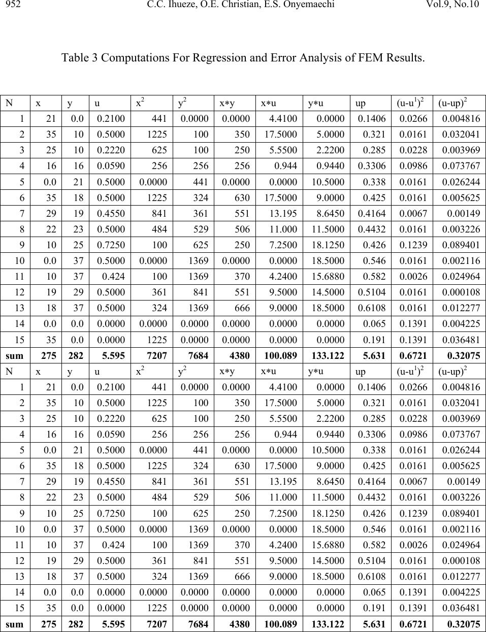 952 C.C. Ihueze, O.E. Christian, E.S. Onyemaechi Vol.9, No.10 Table 3 Computations For Regression and Error Analysis of FEM Results. N x y u x2 y 2 xy xu yu up (u-u1)2 (u-up)2 1 21 0.0 0.2100 441 0.0000 0.0000 4.4100 0.0000 0.1406 0.0266 0.004816 2 35 10 0.5000 1225 100 350 17.5000 5.0000 0.321 0.0161 0.032041 3 25 10 0.2220 625 100 250 5.5500 2.2200 0.285 0.0228 0.003969 4 16 16 0.0590 256 256 256 0.944 0.9440 0.3306 0.0986 0.073767 5 0.0 21 0.5000 0.0000 441 0.0000 0.0000 10.5000 0.338 0.0161 0.026244 6 35 18 0.5000 1225 324 630 17.5000 9.0000 0.425 0.0161 0.005625 7 29 19 0.4550 841 361 551 13.195 8.6450 0.4164 0.0067 0.00149 8 22 23 0.5000 484 529 506 11.000 11.5000 0.4432 0.0161 0.003226 9 10 25 0.7250 100 625 250 7.2500 18.1250 0.426 0.1239 0.089401 10 0.0 37 0.5000 0.0000 1369 0.0000 0.0000 18.5000 0.546 0.0161 0.002116 11 10 37 0.424 100 1369 370 4.2400 15.6880 0.582 0.0026 0.024964 12 19 29 0.5000 361 841 551 9.5000 14.5000 0.5104 0.0161 0.000108 13 18 37 0.5000 324 1369 666 9.0000 18.5000 0.6108 0.0161 0.012277 14 0.0 0.0 0.0000 0.0000 0.0000 0.0000 0.0000 0.0000 0.065 0.1391 0.004225 15 35 0.0 0.0000 1225 0.0000 0.0000 0.0000 0.0000 0.191 0.1391 0.036481 sum 275 282 5.595 7207 7684 4380 100.089 133.122 5.631 0.6721 0.32075 N x y u x2 y 2 xy xu yu up (u-u1)2 (u-up)2 1 21 0.0 0.2100 441 0.0000 0.0000 4.4100 0.0000 0.1406 0.0266 0.004816 2 35 10 0.5000 1225 100 350 17.5000 5.0000 0.321 0.0161 0.032041 3 25 10 0.2220 625 100 250 5.5500 2.2200 0.285 0.0228 0.003969 4 16 16 0.0590 256 256 256 0.944 0.9440 0.3306 0.0986 0.073767 5 0.0 21 0.5000 0.0000 441 0.0000 0.0000 10.5000 0.338 0.0161 0.026244 6 35 18 0.5000 1225 324 630 17.5000 9.0000 0.425 0.0161 0.005625 7 29 19 0.4550 841 361 551 13.195 8.6450 0.4164 0.0067 0.00149 8 22 23 0.5000 484 529 506 11.000 11.5000 0.4432 0.0161 0.003226 9 10 25 0.7250 100 625 250 7.2500 18.1250 0.426 0.1239 0.089401 10 0.0 37 0.5000 0.0000 1369 0.0000 0.0000 18.5000 0.546 0.0161 0.002116 11 10 37 0.424 100 1369 370 4.2400 15.6880 0.582 0.0026 0.024964 12 19 29 0.5000 361 841 551 9.5000 14.5000 0.5104 0.0161 0.000108 13 18 37 0.5000 324 1369 666 9.0000 18.5000 0.6108 0.0161 0.012277 14 0.0 0.0 0.0000 0.0000 0.0000 0.0000 0.0000 0.0000 0.065 0.1391 0.004225 15 35 0.0 0.0000 1225 0.0000 0.0000 0.0000 0.0000 0.191 0.1391 0.036481 sum 275 282 5.595 7207 7684 4380 100.089 133.122 5.631 0.6721 0.32075 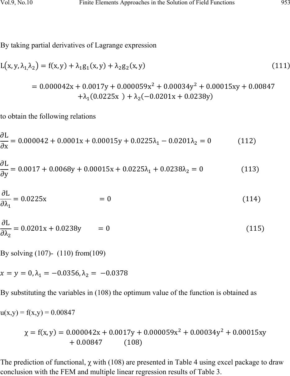 Vol.9, No.10 Finite Elements Approaches in the Solution of Field Functions 953 By taking partial derivatives of Lagrange expression Lx,y,λ,λf x, yλ gx,yλ gx,y 111 0.000042x 0.0017y 0.000059x 0.00034y 0.00015xy 0.00847 λ0.0225x λ 0.0201x 0.0238y to obtain the following relations ∂L ∂x 0.000042 0.0001x 0.00015y 0.0225λ 0.0201λ0 112 ∂L ∂y 0.0017 0.0068y 0.00015x 0.0225λ 0.0238λ0 113 ∂L ∂λ0.0225x 0 114 ∂L ∂λ0.0201x 0.0238y 0 115 By solving (107)- (110) from(109) 0,λ 0.0356, λ 0.0378 By substituting the variables in (108) the optimum value of the function is obtained as u(x,y) = f(x,y) = 0.00847 χf x, y0.000042x 0.0017y 0.000059x 0.00034y 0.00015xy 0.00847 108 The prediction of functional, χ with (108) are presented in Table 4 using excel package to draw conclusion with the FEM and multiple linear regression results of Table 3. 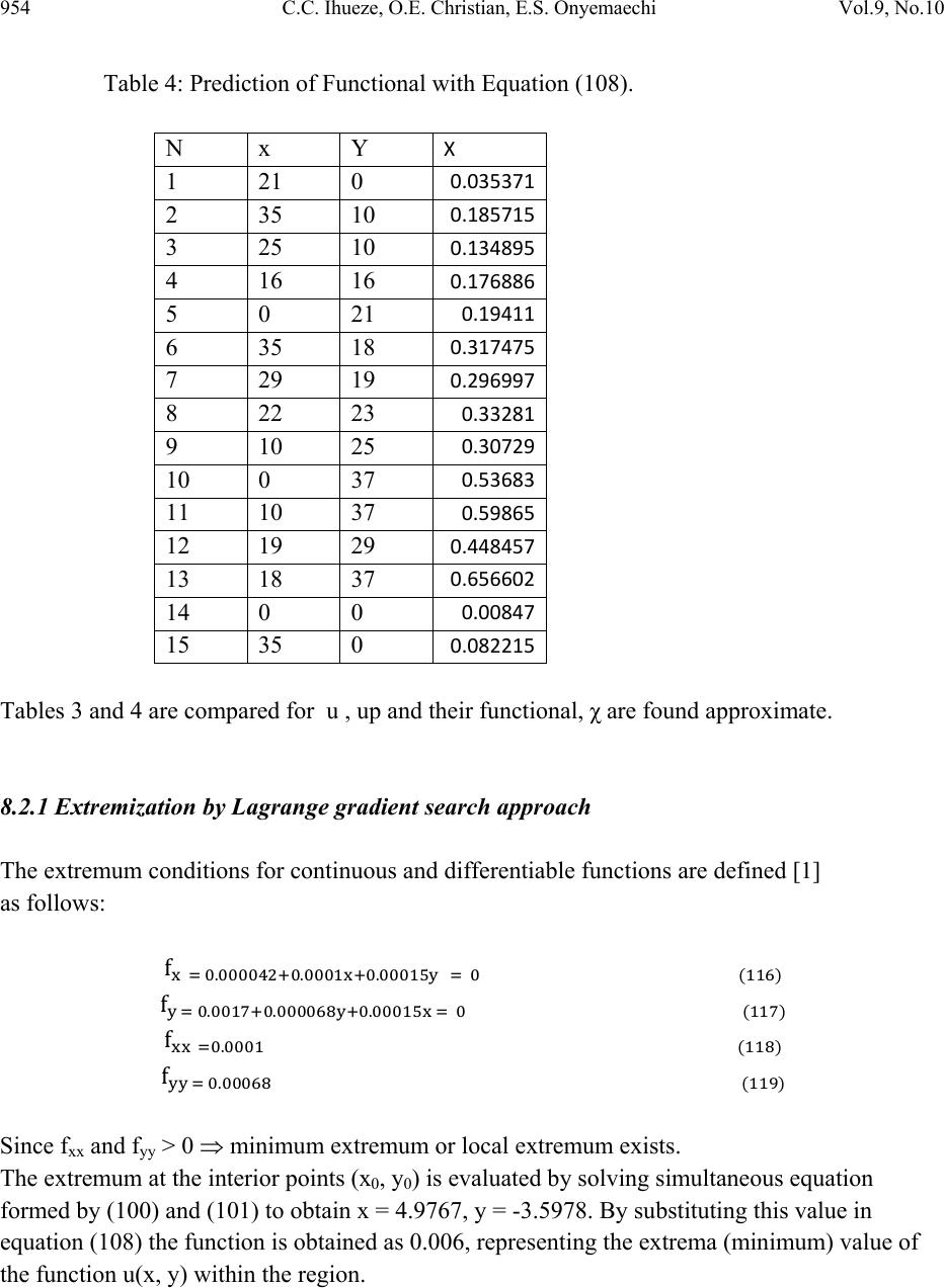 954 C.C. Ihueze, O.E. Christian, E.S. Onyemaechi Vol.9, No.10 Table 4: Prediction of Functional with Equation (108). N x Y Χ 1 21 0 0.035371 2 35 10 0.185715 3 25 10 0.134895 4 16 16 0.176886 5 0 21 0.19411 6 35 18 0.317475 7 29 19 0.296997 8 22 23 0.33281 9 10 25 0.30729 10 0 37 0.53683 11 10 37 0.59865 12 19 29 0.448457 13 18 37 0.656602 14 0 0 0.00847 15 35 0 0.082215 Tables 3 and 4 are compared for u , up and their functional, χ are found approximate. 8.2.1 Extremization by Lagrange gradient search approach The extremum conditions for continuous and differentiable functions are defined [1] as follows: f ... f ... f . f . Since fxx and fyy > 0 minimum extremum or local extremum exists. The extremum at the interior points (x0, y0) is evaluated by solving simultaneous equation formed by (100) and (101) to obtain x = 4.9767, y = -3.5978. By substituting this value in equation (108) the function is obtained as 0.006, representing the extrema (minimum) value of the function u(x, y) within the region.  Vol.9, No.10 Finite Elements Approaches in the Solution of Field Functions 955 8.2.2 Extremization by Lagra nge multipliers approach By expressing (108) in the form fx,y0.000042x 0.0017y 0.000059x 0.00034y 0.00015xy 0.00847 Subject to the constraint relations ux,y0.5 0.0225x 0.5 120 ux,y 0.0201x 0.0238y0 121 derived for nodes 14 and 10 of elements 1 and 5 at the boundaries. By taking partial derivatives of Lagrange expression Lx,y, λ, λx, yλ gx,yλ gx,y 122 0.000042x 0.0017y 0.000059x 0.00034y 0.00015xy 0.00847 λ0.0225x λ 0.0201x 0.0238y to obtain the following relations ∂L ∂x 0.000042 0.0001x 0.00015y 0.0225λ 0.0201λ0 123 ∂L ∂y 0.0017 0.0068y 0.00015x 0.0225λ 0.0238λ0 124 ∂L ∂λ0.0225x 0 125 ∂L ∂λ0.0201x 0.0238y 0 126 By solving (123)- (126) starting from(125) 0,λ 0.0356, λ 0.0378 By substituting the variables in (108) the optimum value of the function is obtained as u(x,y) = f(x,y) = 0.00847.This value compares favourably with the prediction of 0.006 of gradient search method showing agreement with the graphics of Figure 2 and Figure 3. 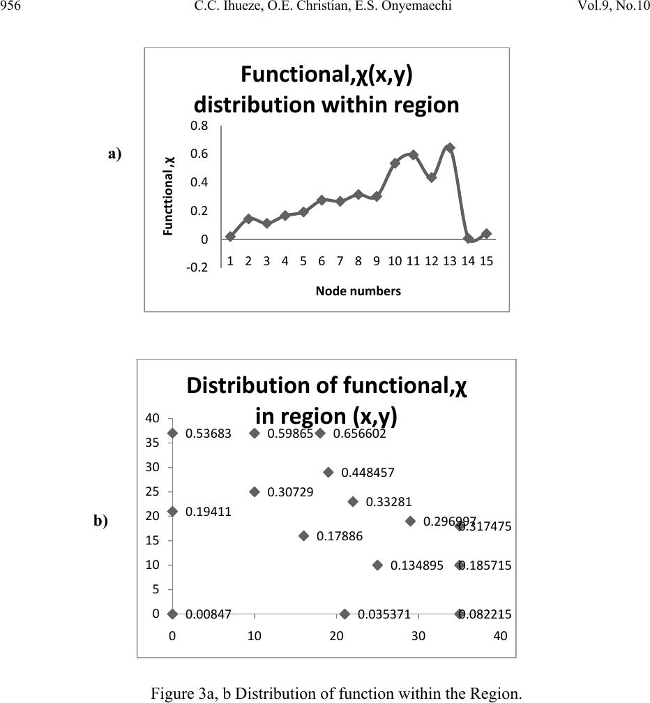 956 C.C. Ihueze, O.E. Christian, E.S. Onyemaechi Vol.9, No.10 Figure 3a, b Distribution of function within the Region. ‐0.2 0 0.2 0.4 0.6 0.8 1 2 3 4 5 6 7 8 9101112131415 Functtional,χ Nodenumbers Functional,χ(x,y) distributionwithinregi o n 0.035371 0.1857150.134895 0.17886 0.19411 0.317475 0.296997 0.33281 0.30729 0.53683 0.59865 0.448457 0.656602 0.00847 0.082215 0 5 10 15 20 25 30 35 40 0 10203040 Distributionoffunctional,χ inregi o n(x,y) b) a) 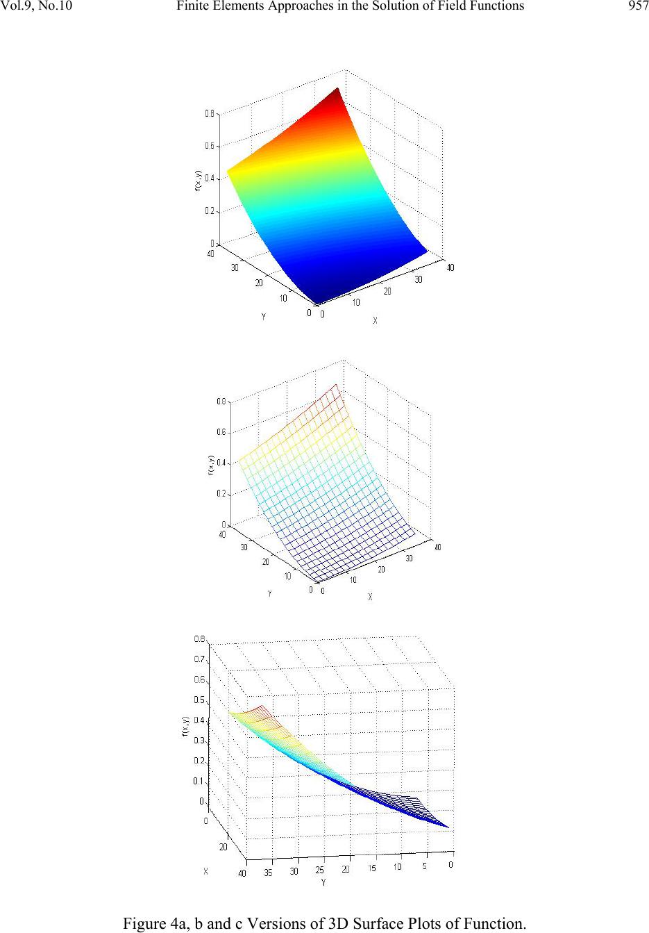 Vol.9, No.10 Finite Elements Approaches in the Solution of Field Functions 957 Figure 4a, b and c Versions of 3D Surface Plots of Function.  958 C.C. Ihueze, O.E. Christian, E.S. Onyemaechi Vol.9, No.10 9. CONCLUSSIONS The methods of this article apply to: 1. Solution of boundary value engineering phenomena whose function can be expressed as partial differential equation. 2. Solution of of displacement in structures and solid mechanics problems, temperature distribution in heat conduction problems, displacement potential in acoustic fluids , pressure in potential flows , velocity in general flows, electric potential in electrostatics magnetic potential in magnetostatics , torsion of non – homogenous shaft, flow through an anisotropic porous foundation, axi – symmetric heat flow, hydrodynamic pressures on moving surfaces 3. Solution of time dependent field problems such as creep, fracture and fatigue. 4. Equations (97) and (98) are recommended for the prediction of possible values of the displacement function of GRP composites region from where other properties of the region could be evaluated. 5. A unified computational model with standard error of 0.15 and correlation coefficient of 0.72 was developed to aid analysis and easy prediction of regional function with which the continuum function was successfully modeled and optimized through gradient search and Lagrange multipliers approach. 6. The MatLab 3-D graphics of Figure 4 show potential trend of function within the regionwith minimum and maximum at the boundaries. REFERENCES [1] Amazigo, J.C and Rubenfield, L.A (1980). Advanced Calculus and its application to the Engineering and Physical Sciences, John Wiley and sons Publishing, New York, pp.130 [2] Zienkiewicz,O.C., and Cheung, Y.K,(1967). The Finite Element in Structural and Continuum Mechanics, McGraw-Hill Publishing Coy Ltd, London, pp.148 [3] Sundaram,V.,Balasubramanian,R.,Lakshminarayanan,K.A.,(2003) Engineering Mathematics, Vol.3,VIKAS Publishing House LTD, New Delhi,pp.173. [4] Ihueze, C. C,Umenwaliri,S.Nand Dara,J.E (2009) Finite Element Approach to Solution of Multidimensional Field Functions, African Research Review: An International Multi- Disciplinary Journal, Vol.3 (5), October, 2009, pp.437-457. [5] Astley, R.J., (1992), Finite Elements in Solids and Structures, Chapman and Hall Publishers, UK, pp.77 [6] Ihueze, C. C. (2010). The Galerki Approach for Finite Elements of Field Functions: The Case of Buckling in GRP. Journal of Minerals and Materials Characterization and Engineering (JMMCE), Vol.9, No.4, pp.389-409  Vol.9, No.10 Finite Elements Approaches in the Solution of Field Functions 959 [7] Ihueze, Chukwutoo. C., (2010). Finite Elements in the Solution of Continuum Field Problems, Journal of Minerals and Materials Characterization and Engineering (JMMCE), Vol.9, No.5.pp.427-452 [8] Canale, R.P and Chapra, S.C (1998), Numerical Methods for Engineers, McGraw-Hill Publishers, 3rd edition, Boston, N.Y,pp.849-853 |