Open Journal of Statistics, 2012, 2, 319-327
http://dx.doi.org/10.4236/ojs.2012.23040 Published Online July 2012 (http://www.SciRP.org/journal/ojs)
A New Method of Construction of Robust Second Order
Slope Rotatable Designs Using Pairwise Balanced Designs
Bejjam Re. Victorbabu, Kottapalli Rajyalakshmi
Department of Statistics, Acharya Nagarjuna University, Guntur, India
Received May 10, 2012; revised June 12, 2012; accepted June 28, 2012
ABSTRACT
In this paper, a new method of construction of robust second order slope rotatable designs (RSOSRD) using pairwise
balanced designs (PBD) is suggested and also obtained the variance of the estimated derivatives for the factors 6 ≤ v ≤
15. It is shown that the new method sometimes leads to designs with less number of design points compared to designs
constructed with the help of balanced incomplete block designs (BIBD).
Keywords: Response Surface Designs; Slope Rotatability; Correlated Errors; Robustness; Second Order Slope
Rotatable Designs (SOSRD)
1. Introduction
In response surface methodology, rotatability is a natural
and highly desirable property. This was introduced and
developed by Box and Hunter [1] assuming the errors to
be uncorrelated and homoscedastic. Das and Narasim-
ham [2] constructed second order rotatable designs (SORD)
through balanced incomplete block designs (BIBD). Tyagi
[3] constructed SORD using pairwise balanced designs
(PBD). Panda and Das [4] studied first order rotatable
designs with correlated errors. In order to study the na-
ture of robust rotatable designs, rotatability conditions
for second order regression designs have been derived,
assuming the errors to be correlated. These conditions
have been further studied under different variance co-
variance structures of errors. Das [5,6] introduced robust
second order rotatable designs (RSORD). Rajyalakshmi
and Victorbabu [7] constructed robust rotatable central
composite designs (RRCCD) for factors 2 ≤ v ≤ 17. Vic-
torbabu and Rajyalakshmi [8] constructed a new method
of construction of robust second order rotatable designs
using BIBD. Victorbabu and Rajyalakshmi [9] studied a
new method of construction of robust second order ro-
tatable designs using PBD.
In response surface methodology, good estimators of
the derivatives of the response function may be as im-
portant or perhaps more important than estimation of
mean response.
Estimation of differences in responses at two different
points in the factor space will often be of great impor-
tance. If a difference in responses at two points close
together is of interest then estimation of local slope (rate
of change) of the response is required. Estimation of
slopes occurs frequently in practical situations. For in-
stance, there are cases in which we want to estimate rate
of reaction in chemical experiment, rate of change in the
yield of a crop to various fertilizer doses, rate of disinte-
gration of radioactive material in animal etc. [9].
Murty and Studden [10] suggested optimal designs for
estimating the slope of a polynomial regression. Hader
and Park [11] introduced slope rotatable central compos-
ite designs assuming errors are uncorrelated and homo-
scedastic. Park [9] studied a class of multifactor designs
for estimating the slope of response surfaces. Victorbabu
and Narasimham [12] constructed second order slope
rotatable designs (SOSRD) using BIBD assuming errors
are uncorrelated and homoscedastic. Victorbabu and Na-
rasimham [13] constructed SOSRD using PBD. Several
authors have studied slope rotatable designs assuming
errors to be uncorrelated and homoscedastic. However it
is not uncommon to come across some practical situa-
tions when the errors are correlated, violating the usual
assumptions. Specifically Das [14] introduced the con-
cept of slope rotatability with correlated errors, which
requires that the variance of the estimated derivative to
be constant, independent of correlation parameter in-
volved in the variance-covariance structure of errors.
They have studied slope rotatability conditions for a
second order design with correlated errors. Victorbabu
and Rajyalakshmi [15] studied robust slope rotatable
central composite designs (RSRCCD) for the factors 2 ≤
v ≤ 8. Further, Victorbabu and Rajyalakshmi [16] studied
robust slope rotatable designs (RSOSRD) using BIBD
for the factors 3 ≤ v ≤ 8.
In this paper, an attempt is made to construct RSO-
C
opyright © 2012 SciRes. OJS

B. RE. VICTORBABU, K. RAJYALAKSHMI 320
SRD using PBD and also obtained the variance of the
estimated derivatives for factors 6 ≤ v ≤ 15.
2. Second Order Response Surface Designs
with Correlated Errors
Assuming that the response surface is of second order,
we adopt the model:
2
0
11
vv
ui iuii iu
ii
Yxx  

 

1
v
ij iujuu
ij
xxe 


,, ,
(2.1)
where xiu denotes the level of the ith factor (i = 1,2, ···, v)
in the uth run (u = 1,2, ···, N) of the experiment, eu’s are
correlated errors. Here 0iiiij

are the parameters
of the model and is the observed response at the uth
design point.
u
Y
Second Order Slope Rotatable Designs with
Correlated Errors
Following Hader and Park [11], Victorbabu and Nara-
simham [12], Das [14], the necessary and sufficient con-
ditions for slope rotatability in second order model with
correlated errors are as follows:
Conditions for Second Order Slope Rotatable Designs
with Correlated Errors.
The estimated response at x is given by
2
0
11
ˆˆ ˆ
ˆ
vv
1
ˆ
v
x
ii ii
ii
iji j
ij
x
xxx 



y  

 
 (2.2)
For the second order model as in (2.2), we have
1; 1
ˆ
v
ij ijj
jj
ˆˆˆ
2
x
ii i
i
x
x 



x
yx


 (2.3)
The variance of ˆ
x
i
x
y
 is given by,
 



The variance of estimated first order derivative with
respect to each independent variable xi as in (2.4) to be a

 
2
2
1;1 1;
1;
1;
.2. .
2.
1;
44
2,
4
ˆˆˆ ˆ
ˆ
ˆˆ
ˆˆ
ˆ
,
44
x
i iii ii
i
vv
,
,
ˆ
ˆˆ
ii
j
ijj s
jjijs jsi
v
jiij
jji
v
i jiiij
jji
i iii iii ii
x
ii
i
ij ij
j
jj
VVxVxCo
x
xV xx
xCov
xxCov
Vvxvxv
x
v
y
x
y

ij is
v
Cov




is
j
1
22
v
iu
i


 




 







 







.
11
..
1; 1;
24
vv
ij
js
ijsjsi
vv
iij iiij
ji
jji jji
xxv
xv xxv
 
 




(2.4)
d


function of
x

if and only if,
..
0;1,0;
iii iij
vivv
1)

 
1, ,ij vij


.0;1 , ij ij
vijjv

2)

 
.0;1 ,, ii ij
vijvij


.constant;1 , ii
viv
3)


.constant;1 , ii ii
viv
4)


.constant 1,and ij ij
vijv 5)
6) ..
1;1 .
4
ii iiij ij
vvijv

 
0.0. 0; 1 jjl jvv v
(2.5)
The following are the equivalent conditions of (1)
through (5) in (2.5) for slope rotatability in secondorre-
lated errors model (2.1).
1)*: a)


.0 ij
v
;

; 1≤ i, j ≤ v, i ≠ j; b)
.0 ii j
v

; 1 ≤ i, j ≤ v; c): i)
.0 ijl
v

; 1 ≤ i, j < l ≤ v; ii)


.. 0 ii jl
v

; 1 ≤ i, j < l ≤ v,

,,jl ii
.. 0 ii jl
v
; iii)



; iv)

1,, ,,,iljtvi jlt 
0.
;
2)*: a)
j
j
v0 a
.ii
v
= constant = , say; 1 ≤ j ≤ v;
b) = constant = 1
e
.ii ii
v
, say; 1 ≤ i ≤ v;
c) = constant = 2
f
g





.ii jj
v
.ij ij
, say; 1 ≤ i ≤ v;
3)*: a) = constant = f; 1 ≤ i ≠ j ≤ v;
b) v = constant = 1; 1 ≤ i < j ≤ v. (2.6)
g
Following (2.6), the necessary and sufficient condi-
tions for second order slope rotatability under the intra-
class structure after some simplifications turn out to be
3 124
1234
1
0;
N
iu iuiu iu
u
xxxx
  

1)*:

4
1
i
i
for any αi odd and



≤
4.
2
1
constant,1
N
iu
u
x
iv

2)*: a)



4
1
constant ,1
N
iu
u
;
x
iv

b)



22
1
constant,, 1,;
N
iu ju
u
;
x
xijvij

3)*



2
2
1
,1
N
iu
u
(2.7)
Using
x
Niv 



22
4
1
,
N
iu ju
u
xx N and





B. RE. VICTORBABU, K. RAJYALAKSHMI
es. OJS
321
1, ,ij vij
 
, the second order slope rotatable design
parameters under the intra-class structure are as follows:
 
Copyright © 2012 SciR
1) 2
11
N
N
02
a



  
;
2)
 

22
42
1
N
N
2
11
11
NN
f







 ;
3)

2
2
1
1
N
e



;
4)

4
2
1
1
N
g




 
;
5) 00211
N
vN

 ;
6)
 
  
22
42
2
113
11 1
NNN
gN
2f


 
 
 
3 124
1234
1
0;
N
iu iuiu iu
u
xxxx
  


4
1
i
i



 . (2.8)
Note that if ρ = 0, the conditions (2.7) and (2.8) re-
duces to
1): for any αi odd and



≤
4.
2): a) 2
2
1
constant ,1
iu
u
;
N
x
Niv 

 
4,1

b) 4
1
constant
N
iu
u
x
cNi v  
41 ,,,


;
3) 22
1
constant
N
iu ju
u
x
xN


ijvij
  (2.9)
where c = 3η, and 4

, 2

, η are constants.
The variances and covariances of the estimated pa-
rameters of the model (2.1) under the slope rotatability
are as follows:
1)


0T

2
ˆ
1
;1
fvf
g
Viv







;1
ˆ;
i
Veiv  

;1
ˆ;Vgijv
 

;
2)
3)
ij
4)
2
00 0
221
,
2
ˆii
vfvfva
g
V
Tff
g

















1;iv



5) 0
0,;;
ˆ1 ˆii
a
Covi v
T







6)
2
000
,;
2
ˆˆ1
ii jj
afv
Covij v
Tff
g












(2.10)
where

2
00 0
21Tvfv fva
g


















ˆ
and other covariance’s are zero.
An inspection of the variance of 0

shows that a
necessary condition for the existence of a non-singular
second order design is T > 0 i.e.,
4)*:

2
00 0
210vfvfva
g






 
 


 


(2.11)
Using (2.8), the expression


2
00 0
21vfvfva
g
















 
simplified to
 

4
2
2
22 2
22
(1)1( 1)
11
(1)
Ncv NN
N
vNvN




  





 
Hence the non-singularity condition is


  



4
22 2
22
111
(1)0
cv NN
vNvN


 

 


(2.12)
For any general second order slope rotatable designs
(c.f. Hader and Park [11]), we have




..
ˆˆ..,
11
44
ii iiij ij
ii ij
VVievv   (2.13)
On simplification of (2.13), using (2.10), we get
5)*:
  
2
0000000 0000
22
41421
f
 
2
0410.
vevfgv fvgvav fgv fvvfg
gg


 
 
  
 

av vfg 
(2.14)
Using (2.8), the condition (2.14) simplifies to

B. RE. VICTORBABU, K. RAJYALAKSHMI 322
 



 

 



 
 
 
 


 

22
42
22 2
42 2
44
22 22
42 42
4
22
2
113
1
113 11
1
42
11 11
11 11
421
111
11
41
NNN
NNN N
N
Nvv
NN
NNNNNNN
vv NN
NN
Nvv


22
42
4
11
NN
N

 


 




 




 


 



  
 







 








22
42
4
0
11
N
NN








(2.15)
For ρ = 0, Equation (2.15) reduces to (see Victorbabu
and Narasimham [12])

22
4
5(3)vcc 




2
54=0vc   

(2.16)
On simplification of Equation (2.4) using Equation
(2.6) and (2.13), we get
22
1;
22
v
ij
jj i
i
xg
x egd








2tk
2k

tk

2tk

22
tk
bvn
1
44
ˆx
i
v
i
g
Vex
x
eg
y







(2.17)
3. New Method of Construction of RSOSRD
Using Pairwise Balanced Designs
Let there be an equi-replicated PBD with parameters (v,
b, r, k1, k2, ···, kp, λ) and k = sup (k1, k2, ···, kp), de-
note a fractional replicate of in ± levels, in which no
interaction with less than five factors is confounded.
[1-(v, b, r, k1, k2, ···, kp, λ)] denote the design points gen-
erated from the transpose of incidence matrix of PBD.
[1-(v, b, r, k1, k2, ···, kp, λ)] are the b design points
generated from PBD (c.f. Raghavarao [17], pp. 298-300)),
n0 denote the number of central points and (±α, 0, 0, ···, 0)
21 denote the design points generated from (±α, 0, 0, ···, 0)
point set.
2
Here we start with usual SOSRD using PBD having
“n” (where n = b + 2v) non-central design points
involving v-factors. For this n-non-central design points
we add (n + 1) (n + n0 = m say) central points in the fol-
lowing way.
One central point is placed in between each pair of
non-central design points in the sequence, resulting
thereby in (n − 1) such central points. The other two cen-
tral points are placed one at the beginning and one at the
end.
If the number of central points of the usual SOSRD
with which we started is greater than (n + 1), the remain-
ing central points are placed in any manner, if the num-
ber is less, we need to include the requisite number of
additional central points. Here we examine the non-sin-
gularity condition for the newly constructed design.
Let N (N = 0



2tk

2tk

2tk 

22
tk
Nb vm
2
) be the number of design
points of an SOSRD using PBD with which we started.
Out of N, let n be the number of non-central design
points and n0 be the number of central points. i.e., N = n
+ n0. Let N1 be the number of design points of the newly
constructed RSOSRD using PBD, where N1 = n + m > N.
For the SOSRD using PBD with which we started, the
following are the moment relations:
Theorem (3.1):
If (v, b, r, k1, k2, ···, kp, λ) is an equi-replicate PB de-
sign and k = sup (k1, k2, ···, kp) denotes a resolution
V fractional replicate of of 2k in ± levels and n0 is the
number of central points, then the design points, [1-(v, b,
r, k1, k2, ···, kp, λ)]  U (α, 0, 0, ···, 0) U(m)
give a v-dimensional RSOSRD in 1
(where m = n + n0) design points, where

is a posi-
tive real root (if it exists) of the biquadratic equation,

 











2
82
1
4
1
2
22
2
22
1
3
2
8482 22
12 24162042
416202
59 62
452 0.
tk tk
tk
tk
tk
tk
vN vrvr
vrN vvr
vrvv r
vvrrN
vrv r







 




  







2
(3.1)
If at least one positive real root of

exists in (3.1)
then the design exists.
c can be obtained from


4
22
2
tk
tv
r
c




122
12
1
2 2constant,
Ntk
iu
u
xr N
. (3.2)
Proof: For the design points generated from the PBD,
simple symmetry conditions 1), 2), 2 of (2.7) are true.
Condition 1) of (2.7) is true obviously. Conditions 2) and
3) of (2.7) are true as follows.
2) a)



 


B. RE. VICTORBABU, K. RAJYALAKSHMI 323
1;iv
14
tant ,cN b)

144
1
2 2cons
Ntk
iu
u
xr

 
1;iv
14
onstant ,N



3)

122
1
2c
Ntk
iu ju
u
xx

 
1ij v
,



(3.3)
From 2) b) and 3) of (3.3), we get c given in (3.2).
Substituting for 24


2
and c in (2.16), and on simplifi-
cation we get the fourth degree equation in

given in
(3.1)
Corollary: If k1 = k2 = ··· = kp = k, then Theorem 3.1
reduces to the method of construction of RSOSRD using
BIBD.
The RSOSRD using pairwise balanced designs values
“α” and the variances of estimated slopes for the factors
6 ≤ v ≤ 15 are given in Appendix.
Example: We illustrate the use of Theorem 3.1 by
constructing a RSOSRD for 6-factors with the help of the
PB design (v = 6, b = 7, r = 3, k1 = 3, k2 = 2, λ = 1).
[1-(6, 7, 3, 3, 2, 1)] × 23 U (α, 0, 0, ···, 0) × 21 U(m =
69) will give a RSOSRD in N1 = 137 design points for
six factors. From (3.3), we have
2) a)
122
1
24 2
N
iu
u
12
,1 ;
x
Niv  
14
,1 ;

 

b)
144
1
24 2
N
iu
u
x
cN

 
i v
 
1 ; 3)
122
14
1
8,
N
iu ju
u
x
xN 


ijv
,
(3.4)
Substituting for 24


2
68352 0  
and c in (2.16), we get the fol-
lowing biquadratic equation.
86 4
500 115264966144    . (3.5)
(3.5) has only one positive real root α2 = 2.7093.
It may be pointed out here that this RSOSRD using
PBD has only 137 design points for 6-factors, where as
the corresponding RSOSRD obtained using a BIB design
(v = 6, b = 10, r = 5, k = 3, λ = 2) needs 185 design points.
Thus the new method sometimes leads to RSO-SRD us-
ing PBD with lesser number of design points than the
RSOSRD obtained through BIB designs.
The Appendix gives the appropriate robust slope rota-
tability values of the parameter “α” for designs using a
PBD, star points and for different number of central
points and also variances and covariances of the factors
for 6 ≤ v ≤ 15.
4. Acknowledgements
The authors are thankful to the referee and the editor for
the valuable suggestions which helped in improving the
quality of the paper.
REFERENCES
[1] G. E. P. Box and J. S. Hunter, “Multifactor Experimental
Designs for Exploring Response Surfaces,” The Annals of
Mathematical Statistics, Vol. 28, No. 1, 1957, pp. 195-
241. doi:10.1214/aoms/1177707047
[2] M. N. Das and V. L. Narasimham, “Construction of Ro-
tatable Designs through Balanced Incomplete Block De-
signs,” Annals of Mathematical Statistics, Vol. 33, No. 4,
1962, pp. 1421-1439.
[3] B. N. Tyagi, “On the Construction of Second Order and
Third Order Rotatable Designs through Pairwise Bal-
anced Designs and Doubly Balanced Designs,” Calcutta
Statistical Association Bulletin, Vol. 13, 1964, pp. 150-
162.
[4] R. N. Panda and R. N. Das, “First Order Rotatable De-
signs with Correlated Errors,” Calcutta Statistical Asso-
ciation Bulletin, Vol. 44, 1994, pp. 83-101.
[5] R. N. Das, “Robust Second Order Rotatable Designs. Part-
I RSORD,” Calcutta Statistical Association Bulletin, Vol.
47, 1997, pp. 199-214.
[6] R. N. Das, “Robust Second Order Rotatable Designs. Part-
II RSORD,” Calcutta Statistical Association Bulletin, Vol.
49, 1999, pp. 65-76.
[7] K. Rajyalakshmi and B. Re. Victorbabu, “Robust Second
Order Rotatable Central Composite Designs,” JP Journal
of Fundamental and Applied Statistics, Vol. 1, No. 2,
2011, pp. 85-102.
[8] B. Re. Victorbabu and K. Rajyalakshmi, “A New Method
of Construction of Robust Second Order Rotatable De-
signs Using Balanced Incomplete Block Designs,” Open
Journal of Statistics, Vol. 2, No. 1, 2012, pp. 39-47.
[9] S. H. Park, “A Class of Multifactor Designs for Estimat-
ing the Slope of Response Surfaces,” Technometrics, Vol.
29, No. 4, 1987, pp. 449-453.
[10] V. N. Murty and W. J. Studden, “Optimal Designs for
Estimating the Slope of a Polynomial Regression,” Jour-
nal of the American Statistical Association, Vol. 67, No.
340, 1972, pp. 869-873.
[11] R. J. Hader and S. H. Park, “Slope-Rotatable Central Com-
posite Designs,” Technometrics, Vol. 20, No. 4, 1978, pp.
413-417.
[12] B. Re. Victorbabu and V. L. Narasimham, “Construction
of Second Order Slope Rotatable Designs through Bal-
anced Incomplete Block Designs,” Communications in
Statistics—Theory and Methods, Vol. 20, No. 8, 1991, pp.
2467-2478. doi:10.1080/03610929108830644
[13] B. Re. Victorbabu and V. L. Narasimham, “Construction
of Second Order Slope Rotatable Designs Using Pairwise
Balanced Designs,” Journal of the Indian Society of Ag-
ricultural Statistics, Vol. 45, No. 2, 1993, pp. 200-205.
[14] R. N. Das, “Slope Rotatability with Correlated Errors,”
Calcutta Statistical Association Bulletin, Vol. 54, 2003,
pp. 57-70.

B. RE. VICTORBABU, K. RAJYALAKSHMI 324
[15] B. Re. Victorbabu and K. Rajyalakshmi, “Robust Slope
Rotatable Central Composite Designs,” Paper Submitted
for the Possible Publication, 2012.
[16] B. Re. Victorbabu and K. Rajyalakshmi, “Robust Second
Order Slope Rotatable Designs Using Balanced Incom-
plete Block Designs,” Paper Submitted for the Possible
Publication, 2012.
[17] D. Raghavarao, “Constructions and Combinatorial Prob-
lems in Design of Experiments,” John Wiley and Sons,
New York, 1971.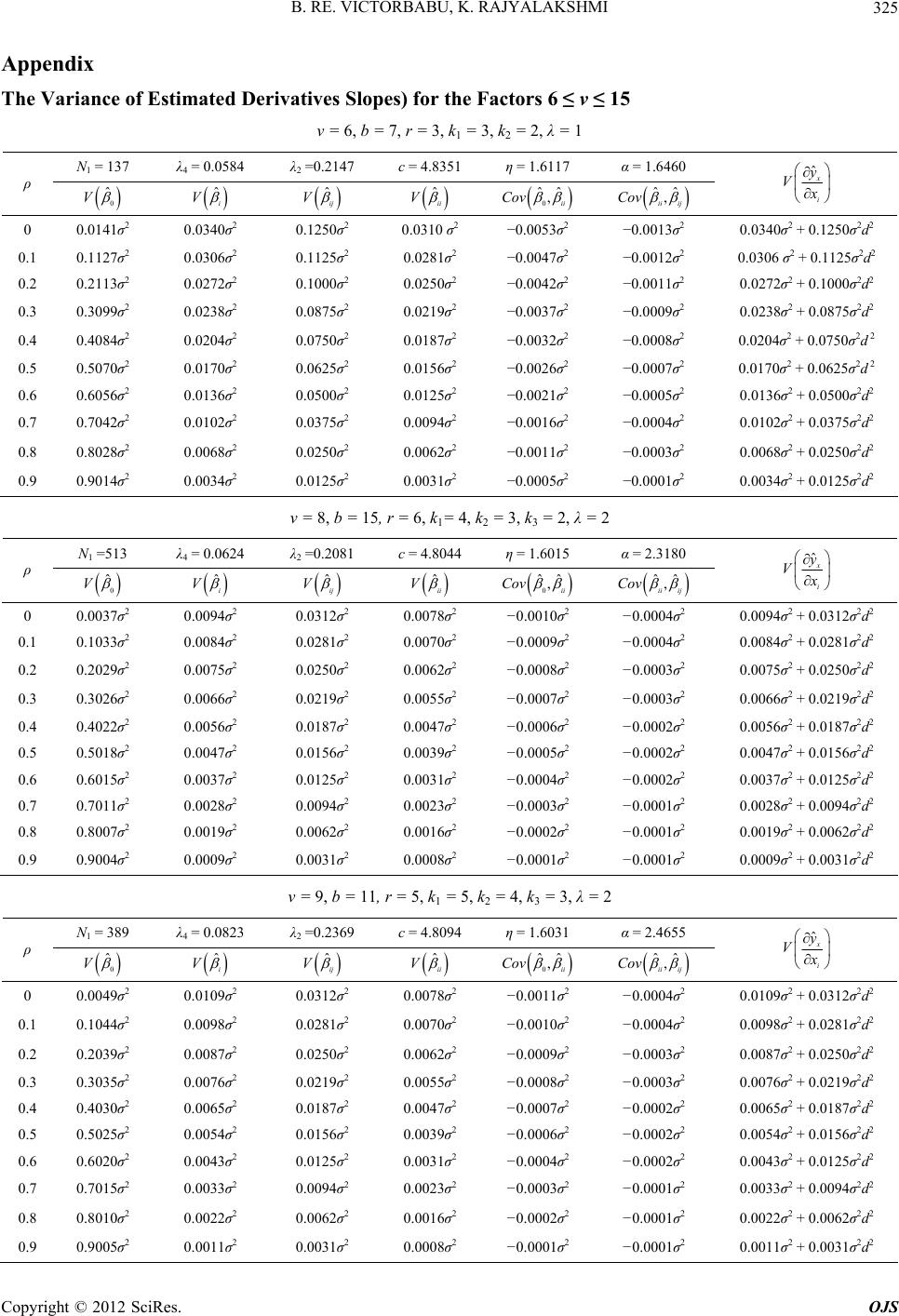

B. RE. VICTORBABU, K. RAJYALAKSHMI 325
Appendix
The Variance of Estimated Derivatives Slopes) for the Factors 6 ≤ v ≤ 15
v = 6, b = 7, r = 3, k1 = 3, k2 = 2, λ = 1
N1 = 137 λ4 = 0.0584 λ2 =0.2147 c = 4.8351 η = 1.6117 α = 1.6460
ρ

0
ˆ
V


ˆi
V


ˆij
V



ˆii
V



0,
ˆˆii
Cov




ˆij
ˆx
i
ˆ,
ii
Cov
x
y
V






0 0.0141σ2 0.0340σ2 0.1250σ2 0.0310 σ2 −0.0053σ2 −0.0013σ2 0.0340σ2 + 0.1250σ2d2
0.1 0.1127σ2 0.0306σ2 0.1125σ2 0.0281σ2 −0.0047σ2 −0.0012σ2 0.0306 σ2 + 0.1125σ2d2
0.2 0.2113σ2 0.0272σ2 0.1000σ2 0.0250σ2 −0.0042σ2 −0.0011σ2 0.0272σ2 + 0.1000σ2d2
0.3 0.3099σ2 0.0238σ2 0.0875σ2 0.0219σ2 −0.0037σ2 −0.0009σ2 0.0238σ2 + 0.0875σ2d2
0.4 0.4084σ2 0.0204σ2 0.0750σ2 0.0187σ2 −0.0032σ2 −0.0008σ2 0.0204σ2 + 0.0750σ2d 2
0.5 0.5070σ2 0.0170σ2 0.0625σ2 0.0156σ2 −0.0026σ2 −0.0007σ2 0.0170σ2 + 0.0625σ2d 2
0.6 0.6056σ2 0.0136σ2 0.0500σ2 0.0125σ2 −0.0021σ2 −0.0005σ2 0.0136σ2 + 0.0500σ2d2
0.7 0.7042σ2 0.0102σ2 0.0375σ2 0.0094σ2 −0.0016σ2 −0.0004σ2 0.0102σ2 + 0.0375σ2d2
0.8 0.8028σ2 0.0068σ2 0.0250σ2 0.0062σ2 −0.0011σ2 −0.0003σ2 0.0068σ2 + 0.0250σ2d2
0.9 0.9014σ2 0.0034σ2 0.0125σ2 0.0031σ2 −0.0005σ2 −0.0001σ2 0.0034σ2 + 0.0125σ2d2
v = 8, b = 15, r = 6, k1= 4, k2 = 3, k3 = 2, λ = 2
N1 =513 λ4 = 0.0624 λ2 =0.2081 c = 4.8044 η = 1.6015 α = 2.3180
ρ

0
ˆ
V


ˆi
V


ˆij
V



ˆii
V



0,
ˆˆii
Cov




ˆij
ˆx
i
ˆ,
ii
Cov
x
y
V






0 0.0037σ2 0.0094σ2 0.0312σ2 0.0078σ2 −0.0010σ2 −0.0004σ2 0.0094σ2 + 0.0312σ2d2
0.1 0.1033σ2 0.0084σ2 0.0281σ2 0.0070σ2 −0.0009σ2 −0.0004σ2 0.0084σ2 + 0.0281σ2d2
0.2 0.2029σ2 0.0075σ2 0.0250σ2 0.0062σ2 −0.0008σ2 −0.0003σ2 0.0075σ2 + 0.0250σ2d2
0.3 0.3026σ2 0.0066σ2 0.0219σ2 0.0055σ2 −0.0007σ2 −0.0003σ2 0.0066σ2 + 0.0219σ2d2
0.4 0.4022σ2 0.0056σ2 0.0187σ2 0.0047σ2 −0.0006σ2 −0.0002σ2 0.0056σ2 + 0.0187σ2d2
0.5 0.5018σ2 0.0047σ2 0.0156σ2 0.0039σ2 −0.0005σ2 −0.0002σ2 0.0047σ2 + 0.0156σ2d2
0.6 0.6015σ2 0.0037σ2 0.0125σ2 0.0031σ2 −0.0004σ2 −0.0002σ2 0.0037σ2 + 0.0125σ2d2
0.7 0.7011σ2 0.0028σ2 0.0094σ2 0.0023σ2 −0.0003σ2 −0.0001σ2 0.0028σ2 + 0.0094σ2d2
0.8 0.8007σ2 0.0019σ2 0.0062σ2 0.0016σ2 −0.0002σ2 −0.0001σ2 0.0019σ2 + 0.0062σ2d2
0.9 0.9004σ2 0.0009σ2 0.0031σ2 0.0008σ2 −0.0001σ2 −0.0001σ2 0.0009σ2 + 0.0031σ2d2
v = 9, b = 11, r = 5, k1 = 5, k2 = 4, k3 = 3, λ = 2
N1 = 389 λ4 = 0.0823 λ2 =0.2369 c = 4.8094 η = 1.6031 α = 2.4655
ρ

0
ˆ
V


ˆi
V


ˆij
V



ˆii
V



0,
ˆˆii
Cov




ˆij
ˆx
i
ˆ,
ii
Cov
x
y
V






0 0.0049σ2 0.0109σ2 0.0312σ2 0.0078σ2 −0.0011σ2 −0.0004σ2 0.0109σ2 + 0.0312σ2d2
0.1 0.1044σ2 0.0098σ2 0.0281σ2 0.0070σ2 −0.0010σ2 −0.0004σ2 0.0098σ2 + 0.0281σ2d2
0.2 0.2039σ2 0.0087σ2 0.0250σ2 0.0062σ2 −0.0009σ2 −0.0003σ2 0.0087σ2 + 0.0250σ2d2
0.3 0.3035σ2 0.0076σ2 0.0219σ2 0.0055σ2 −0.0008σ2 −0.0003σ2 0.0076σ2 + 0.0219σ2d2
0.4 0.4030σ2 0.0065σ2 0.0187σ2 0.0047σ2 −0.0007σ2 −0.0002σ2 0.0065σ2 + 0.0187σ2d2
0.5 0.5025σ2 0.0054σ2 0.0156σ2 0.0039σ2 −0.0006σ2 −0.0002σ2 0.0054σ2 + 0.0156σ2d2
0.6 0.6020σ2 0.0043σ2 0.0125σ2 0.0031σ2 −0.0004σ2 −0.0002σ2 0.0043σ2 + 0.0125σ2d2
0.7 0.7015σ2 0.0033σ2 0.0094σ2 0.0023σ2 −0.0003σ2 −0.0001σ2 0.0033σ2 + 0.0094σ2d2
0.8 0.8010σ2 0.0022σ2 0.0062σ2 0.0016σ2 −0.0002σ2 −0.0001σ2 0.0022σ2 + 0.0062σ2d2
0.9 0.9005σ2 0.0011σ2 0.0031σ2 0.0008σ2 −0.0001σ2 −0.0001σ2 0.0011σ2 + 0.0031σ2d2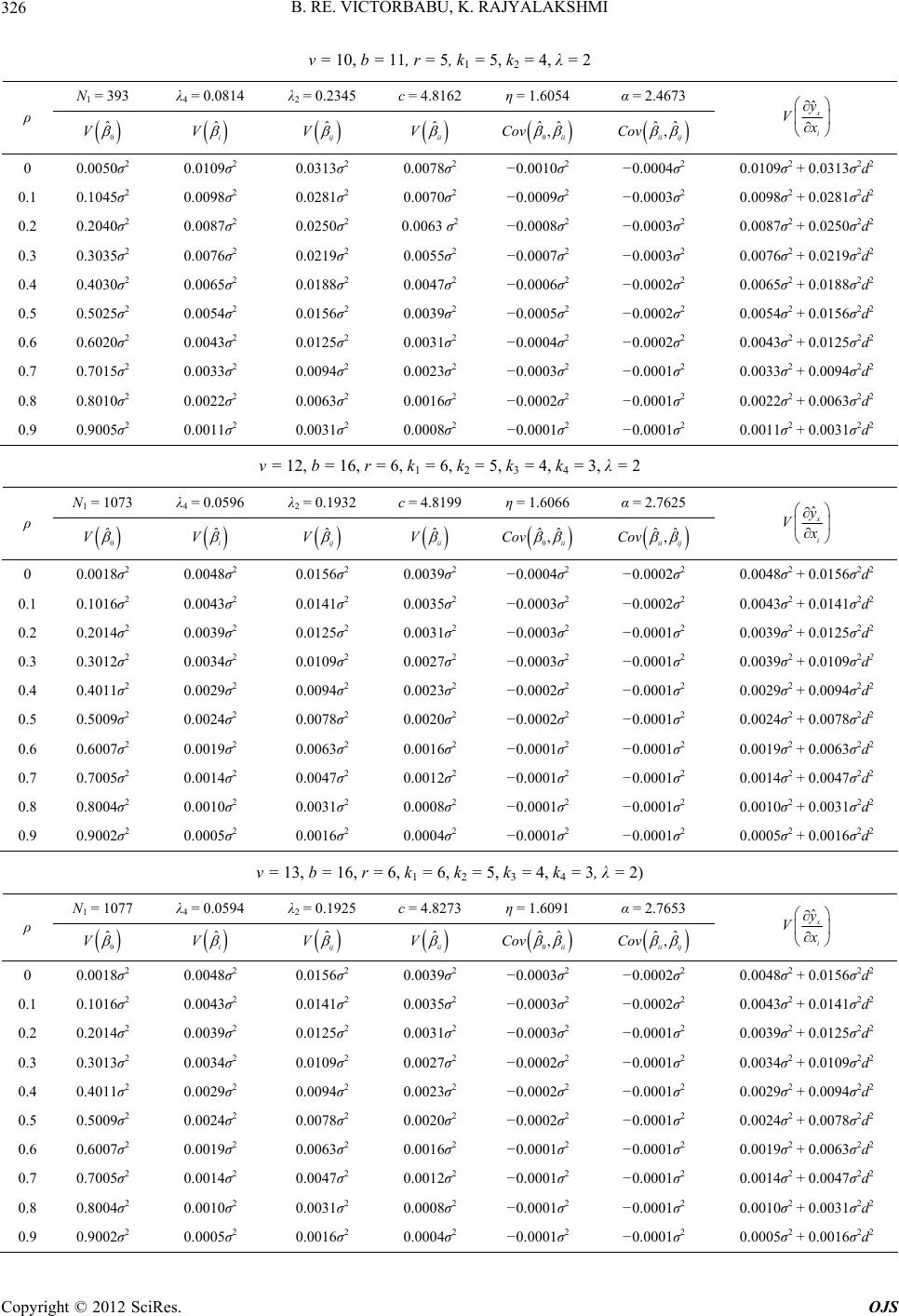

B. RE. VICTORBABU, K. RAJYALAKSHMI 326
v = 10, b = 11, r = 5, k1 = 5, k2 = 4, λ = 2
N1 = 393 λ4 = 0.0814 λ2 = 0.2345 c = 4.8162 η = 1.6054 α = 2.4673
ρ

0
ˆ
V


ˆi
V


ˆij
V



ˆii
V



0,
ˆˆii
Cov




ˆij
ˆx
i
ˆ,
ii
Cov
x
y
V






0 0.0050σ2 0.0109σ2 0.0313σ2 0.0078σ2 −0.0010σ2 −0.0004σ2 0.0109σ2 + 0.0313σ2d2
0.1 0.1045σ2 0.0098σ2 0.0281σ2 0.0070σ2 −0.0009σ2 −0.0003σ2 0.0098σ2 + 0.0281σ2d2
0.2 0.2040σ2 0.0087σ2 0.0250σ2 0.0063 σ2 −0.0008σ2 −0.0003σ2 0.0087σ2 + 0.0250σ2d2
0.3 0.3035σ2 0.0076σ2 0.0219σ2 0.0055σ2 −0.0007σ2 −0.0003σ2 0.0076σ2 + 0.0219σ2d2
0.4 0.4030σ2 0.0065σ2 0.0188σ2 0.0047σ2 −0.0006σ2 −0.0002σ2 0.0065σ2 + 0.0188σ2d2
0.5 0.5025σ2 0.0054σ2 0.0156σ2 0.0039σ2 −0.0005σ2 −0.0002σ2 0.0054σ2 + 0.0156σ2d2
0.6 0.6020σ2 0.0043σ2 0.0125σ2 0.0031σ2 −0.0004σ2 −0.0002σ2 0.0043σ2 + 0.0125σ2d2
0.7 0.7015σ2 0.0033σ2 0.0094σ2 0.0023σ2 −0.0003σ2 −0.0001σ2 0.0033σ2 + 0.0094σ2d2
0.8 0.8010σ2 0.0022σ2 0.0063σ2 0.0016σ2 −0.0002σ2 −0.0001σ2 0.0022σ2 + 0.0063σ2d2
0.9 0.9005σ2 0.0011σ2 0.0031σ2 0.0008σ2 −0.0001σ2 −0.0001σ2 0.0011σ2 + 0.0031σ2d2
v = 12, b = 16, r = 6, k1 = 6, k2 = 5, k3 = 4, k4 = 3, λ = 2
N1 = 1073 λ4 = 0.0596 λ2 = 0.1932 c = 4.8199 η = 1.6066 α = 2.7625
ρ

0
ˆ
V


ˆi
V


ˆij
V



ˆii
V



0,
ˆˆii
Cov




ˆij
ˆx
i
ˆ,
ii
Cov
x
y
V






0 0.0018σ2 0.0048σ2 0.0156σ2 0.0039σ2 −0.0004σ2 −0.0002σ2 0.0048σ2 + 0.0156σ2d2
0.1 0.1016σ2 0.0043σ2 0.0141σ2 0.0035σ2 −0.0003σ2 −0.0002σ2 0.0043σ2 + 0.0141σ2d2
0.2 0.2014σ2 0.0039σ2 0.0125σ2 0.0031σ2 −0.0003σ2 −0.0001σ2 0.0039σ2 + 0.0125σ2d2
0.3 0.3012σ2 0.0034σ2 0.0109σ2 0.0027σ2 −0.0003σ2 −0.0001σ2 0.0039σ2 + 0.0109σ2d2
0.4 0.4011σ2 0.0029σ2 0.0094σ2 0.0023σ2 −0.0002σ2 −0.0001σ2 0.0029σ2 + 0.0094σ2d2
0.5 0.5009σ2 0.0024σ2 0.0078σ2 0.0020σ2 −0.0002σ2 −0.0001σ2 0.0024σ2 + 0.0078σ2d2
0.6 0.6007σ2 0.0019σ2 0.0063σ2 0.0016σ2 −0.0001σ2 −0.0001σ2 0.0019σ2 + 0.0063σ2d2
0.7 0.7005σ2 0.0014σ2 0.0047σ2 0.0012σ2 −0.0001σ2 −0.0001σ2 0.0014σ2 + 0.0047σ2d2
0.8 0.8004σ2 0.0010σ2 0.0031σ2 0.0008σ2 −0.0001σ2 −0.0001σ2 0.0010σ2 + 0.0031σ2d2
0.9 0.9002σ2 0.0005σ2 0.0016σ2 0.0004σ2 −0.0001σ2 −0.0001σ2 0.0005σ2 + 0.0016σ2d2
v = 13, b = 16, r = 6, k1 = 6, k2 = 5, k3 = 4, k4 = 3, λ = 2)
N1 = 1077 λ4 = 0.0594 λ2 = 0.1925 c = 4.8273 η = 1.6091 α = 2.7653
ρ

0
ˆ
V


ˆi
V


ˆij
V



ˆii
V



0,
ˆˆii
Cov




ˆij
ˆx
i
ˆ,
ii
Cov
x
y
V






0 0.0018σ2 0.0048σ2 0.0156σ2 0.0039σ2 −0.0003σ2 −0.0002σ2 0.0048σ2 + 0.0156σ2d2
0.1 0.1016σ2 0.0043σ2 0.0141σ2 0.0035σ2 −0.0003σ2 −0.0002σ2 0.0043σ2 + 0.0141σ2d2
0.2 0.2014σ2 0.0039σ2 0.0125σ2 0.0031σ2 −0.0003σ2 −0.0001σ2 0.0039σ2 + 0.0125σ2d2
0.3 0.3013σ2 0.0034σ2 0.0109σ2 0.0027σ2 −0.0002σ2 −0.0001σ2 0.0034σ2 + 0.0109σ2d2
0.4 0.4011σ2 0.0029σ2 0.0094σ2 0.0023σ2 −0.0002σ2 −0.0001σ2 0.0029σ2 + 0.0094σ2d2
0.5 0.5009σ2 0.0024σ2 0.0078σ2 0.0020σ2 −0.0002σ2 −0.0001σ2 0.0024σ2 + 0.0078σ2d2
0.6 0.6007σ2 0.0019σ2 0.0063σ2 0.0016σ2 −0.0001σ2 −0.0001σ2 0.0019σ2 + 0.0063σ2d2
0.7 0.7005σ2 0.0014σ2 0.0047σ2 0.0012σ2 −0.0001σ2 −0.0001σ2 0.0014σ2 + 0.0047σ2d2
0.8 0.8004σ2 0.0010σ2 0.0031σ2 0.0008σ2 −0.0001σ2 −0.0001σ2 0.0010σ2 + 0.0031σ2d2
0.9 0.9002σ2 0.0005σ2 0.0016σ2 0.0004σ2 −0.0001σ2 −0.0001σ2 0.0005σ2 + 0.0016σ2d2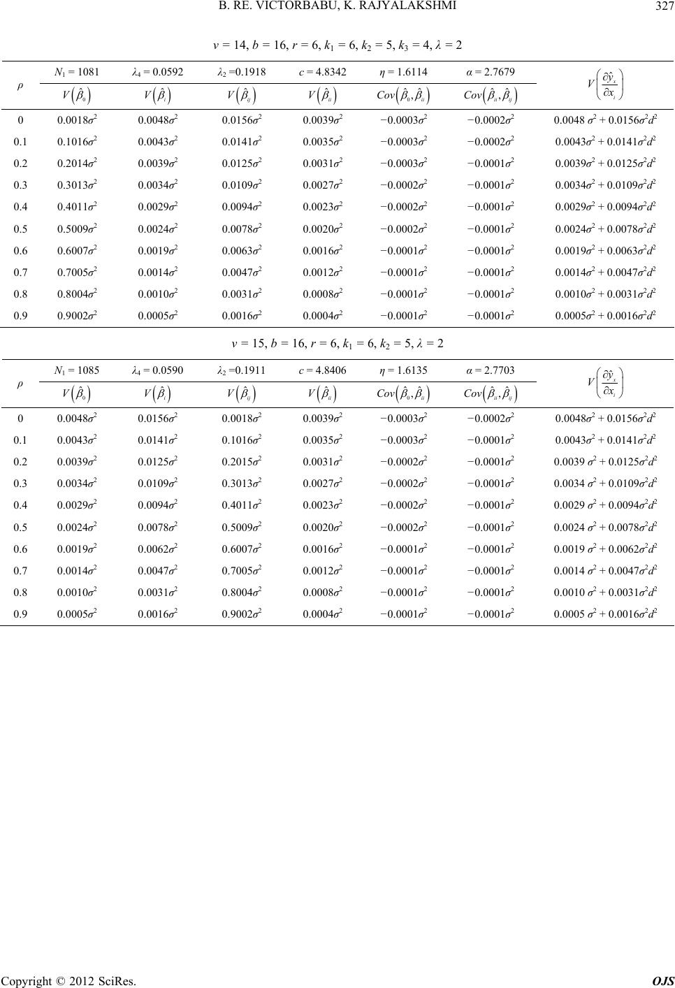

B. RE. VICTORBABU, K. RAJYALAKSHMI 327
v = 14, b = 16, r = 6, k1 = 6, k2 = 5, k3 = 4, λ = 2
N1 = 1081 λ4 = 0.0592 λ2 =0.1918 c = 4.8342 η = 1.6114 α = 2.7679
ρ

0
ˆ
V


ˆi
V


ˆij
V



ˆii
V



0,
ˆˆii
Cov




ˆij
ˆx
i
ˆ,
ii
Cov
x
y
V






0 0.0018σ2 0.0048σ2 0.0156σ2 0.0039σ2 −0.0003σ2 −0.0002σ2 0.0048 σ2 + 0.0156σ2d2
0.1 0.1016σ2 0.0043σ2 0.0141σ2 0.0035σ2 −0.0003σ2 −0.0002σ2 0.0043σ2 + 0.0141σ2d2
0.2 0.2014σ2 0.0039σ2 0.0125σ2 0.0031σ2 −0.0003σ2 −0.0001σ2 0.0039σ2 + 0.0125σ2d2
0.3 0.3013σ2 0.0034σ2 0.0109σ2 0.0027σ2 −0.0002σ2 −0.0001σ2 0.0034σ2 + 0.0109σ2d2
0.4 0.4011σ2 0.0029σ2 0.0094σ2 0.0023σ2 −0.0002σ2 −0.0001σ2 0.0029σ2 + 0.0094σ2d2
0.5 0.5009σ2 0.0024σ2 0.0078σ2 0.0020σ2 −0.0002σ2 −0.0001σ2 0.0024σ2 + 0.0078σ2d2
0.6 0.6007σ2 0.0019σ2 0.0063σ2 0.0016σ2 −0.0001σ2 −0.0001σ2 0.0019σ2 + 0.0063σ2d2
0.7 0.7005σ2 0.0014σ2 0.0047σ2 0.0012σ2 −0.0001σ2 −0.0001σ2 0.0014σ2 + 0.0047σ2d2
0.8 0.8004σ2 0.0010σ2 0.0031σ2 0.0008σ2 −0.0001σ2 −0.0001σ2 0.0010σ2 + 0.0031σ2d2
0.9 0.9002σ2 0.0005σ2 0.0016σ2 0.0004σ2 −0.0001σ2 −0.0001σ2 0.0005σ2 + 0.0016σ2d2
v = 15, b = 16, r = 6, k1 = 6, k2 = 5, λ = 2
N1 = 1085 λ4 = 0.0590 λ2 =0.1911 c = 4.8406 η = 1.6135 α = 2.7703
ρ

0
ˆ
V


ˆi
V


ˆij
V



ˆii
V



0,
ˆˆii
Cov




ˆij
ˆx
i
ˆ,
ii
Cov
x
y
V






0 0.0048σ2 0.0156σ2 0.0018σ2 0.0039σ2 −0.0003σ2 −0.0002σ2 0.0048σ2 + 0.0156σ2d2
0.1 0.0043σ2 0.0141σ2 0.1016σ2 0.0035σ2 −0.0003σ2 −0.0001σ2 0.0043σ2 + 0.0141σ2d2
0.2 0.0039σ2 0.0125σ2 0.2015σ2 0.0031σ2 −0.0002σ2 −0.0001σ2 0.0039 σ2 + 0.0125σ2d2
0.3 0.0034σ2 0.0109σ2 0.3013σ2 0.0027σ2 −0.0002σ2 −0.0001σ2 0.0034 σ2 + 0.0109σ2d2
0.4 0.0029σ2 0.0094σ2 0.4011σ2 0.0023σ2 −0.0002σ2 −0.0001σ2 0.0029 σ2 + 0.0094σ2d2
0.5 0.0024σ2 0.0078σ2 0.5009σ2 0.0020σ2 −0.0002σ2 −0.0001σ2 0.0024 σ2 + 0.0078σ2d2
0.6 0.0019σ2 0.0062σ2 0.6007σ2 0.0016σ2 −0.0001σ2 −0.0001σ2 0.0019 σ2 + 0.0062σ2d2
0.7 0.0014σ2 0.0047σ2 0.7005σ2 0.0012σ2 −0.0001σ2 −0.0001σ2 0.0014 σ2 + 0.0047σ2d2
0.8 0.0010σ2 0.0031σ2 0.8004σ2 0.0008σ2 −0.0001σ2 −0.0001σ2 0.0010 σ2 + 0.0031σ2d2
0.9 0.0005σ2 0.0016σ2 0.9002σ2 0.0004σ2 −0.0001σ2 −0.0001σ2 0.0005 σ2 + 0.0016σ2d2