Open Journal of Statistics, 2012, 2, 328-345
http://dx.doi.org/10.4236/ojs.2012.23041 Published Online July 2012 (http://www.SciRP.org/journal/ojs)
Statistical Comparison of Eight Alternative Methods for
the Analysis of Paired Sample Data with Applications
Godday Uwawunkonye Ebuh*, Ikewelugo Cyprian Anaene Oyeka
Department of Statistics, Faculty of Physical Sciences, Nnamdi Azikiwe University,
Awka, Nigeria
Received March 8, 2012; revised June 10, 2012; accepted June 24, 2012
ABSTRACT
This paper presents and statistically compares eight alternative methods that could possibly be used in the analysis of
matched or paired sample data, including situations in which the data being analyzed satisfy the usual assumptions of
normality and continuity necessary for the use of parametric tests as well as when the data are numeric and non-numeric
measurements on as low as the ordinal scale. It is shown that only the modified sign tests based on only the raw obser-
vations or their assigned ranks may be used with non numeric measurement on the ordinal scale. If the ordinary sign test,
the Wilcoxon signed rank sum test and the modified sign tests can be equally used in data analysis, then it is shown that
the modified sign tests are more efficient and hence more powerful than the ordinary sign tests because the two test sta-
tistics are intrinsically and structurally modified for the possible presence of tied observations between the sampled
populations for both using raw and simulated data. Of all the non-parametric methods presented, the modified Wil-
coxon’s signed rank sum test when applicable is the most efficient and powerful, followed in this order by the modified
sign test by ranks and the modified sign test based on only raw scores for raw data while using simulation, modified
sign test by ranks is the most efficient and powerful, followed in this order by modified Wilcoxon’s signed rank sum
test and modified sign test. Each of the non-parametric methods presented can be easily modified and re-specified for
use with one sample data by simply re-designating the observations from one of the sampled populations to correspond
with a hypothesized value of some measure of central tendency. The methods are illustrated with some raw data as well
as simulated data and their relative performances compared.
Keywords: Normality; Continuity; Paired Sample; Parametric Test; Nonparametric; Numeric; Relative Performance;
Tied Observation
1. Introduction
A clinician, medical researcher or research scientist may
expose a random sample of subjects to some treatment or
drug at two points in time or space, or expose two ran-
dom samples of subjects matched on several characteris-
tics, one to an active or new drug or treatment, and the
other to a diluent, inactive placebo or control treatment
and research interest is in comparing the responses after
the exposure. A dietician may be interested in studying a
random sample of subjects, treated with a regimen of diet
or exercises and in measuring their responses in terms of
the differences between body weights before and after
the experiences. A panel of judges or examiners may be
interested in comparing the performances of candidates
in two tests or examinations taken at two points in time
or space. A psychologist or psychiatrist may wish to
compare the performance of two matched samples of
subjects exposed to two experimental conditions. A
beautician, marketing consultant or advertising agent,
product promoter or investor may wish to compare the
performance of a line of products in terms of their ac-
ceptability or sales, at two different points in time or
space, etc.
In each of these and similar situations, the researcher
may wish to select a statistical method often used in the
analysis of matched or paired samples that is relatively
efficient and powerful in terms of being able to more
readily reject a false null hypothesis and accept a true
one and hence be able to reach more reliable conclusions.
This paper presents, discusses and compares eight al-
ternative statistical methods that may be used for this
purpose.
2. The Proposed Methods
Let (xi1, xi2) be the ith pair randomly drawn from popula-
tions X1 and X2, for i = 1,2, ···, n. Populations X1 and X2
*Corresponding author.
C
opyright © 2012 SciRes. OJS

G. U. EBUH, I. C. A. OYEKA 329
may or may not be measurements that are continuous;
normally distributed; numeric data; independent; but they
should be measurements on at least the ordinal scale.
Interest is in statistically comparing the following eight
methods for analyzing paired samples. They include
paired sample t test, ordinary sign test for two samples,
exact binomial test, normal approximation to the ordi-
nary two sample sign test, unmodified Wilcoxon signed
rank sum test for paired samples, modified sign test,
modified sign test by ranks, and modified Wilcoxon
signed rank sum test for paired samples.
All modifications or adjustments of test statistics are
aimed at adjusting and making provisions for the possi-
bility of any ties, that is tied observations between sam-
pled populations and hence obviate the need to require
the sampled populations to be continuous or even nu-
meric.
2.1. Paired Sample T Test
Required Assumptions
Populations continuous and normally distributed; or sam-
ple size sufficiently large [1]. This method can only be
used for data that satisfy the required assumptions and
are measurements on at least the interval scale.
Let
12iii
dxx (1.1)
for i = 1, 2, ···, n.
Let 1
n
i
di
dn

 be the mean value of the differences
and
2
1
1
n
i
di
n
in





 






22
1
n
di
sd


 (1.2)
Be the variance of the differences.
Let:

Sd
Se dn  (1.3)
be the standard deviation of the mean difference d
10
s :
d
. We
want to test the null hypothesis
00
: v
d
H
dH d

  (1.4)
where d0 is any real number including zero. The test sta-
tistic is [1].
0
d
dd
tSn

 (1.5)
which has a t distribution with n – 1 degrees of free-
dom .We reject H0 at the  level of significance if
1/2; 1
n tt




12iii
dx x
(1.6)
Otherwise H0 is accepted.
2.2. Ordinary Sign Test for Two Samples
Required Assumptions
Populations continuous and numeric measurements.
The test statistic is based on the signs (+ sign, or – sign)
of the differences between members of the paired sample
observations.
Thus let


1
1, if0
0, if0
i
ii
d
ud




d
(2.1)
for i = 1, 2, ···, n.
Let
(2.2)
for i = 1, 2, ···, n.
Note that Equation (2.1) assumes that there are no ties
that is i cannot be 0 and hence does not make any
provisions for this possibility.
Let


1
i
pu



1
n
i
i
Wu


(2.3)
Let
(2.4)
It is easily shown [2] that


.; 1EWn VarWn




00 10
:0.50 vs :0.50HH
(2.5)
The test statistics for the null hypothesis of equal
population medians
(H0: M1 = M2 = M0), that is of the null hypothesis,






(2.6)
In general


22
00 2
00
1
wn wn
Var wn







22
1:1
(2.7)
which has the chi-square distribution with 1 degree of
freedom for sufficiently large n.
H0 is rejected at the  level of significance if



 (2.8)
Otherwise H0 is accepted.
Note that in particular under the null hypothesis usu-
ally tested in the sign test (H0:  = 
0 = 0.50) Equation
(2.7) reduces to

G. U. EBUH, I. C. A. OYEKA 330

2
0.5
0.25
wn
n


12
12
12
if
if
if
ii
ii
ii
2
 (2.9)
which has the chi-square distribution with 1 degree of
freedom, if n is sufficiently large.
2.3. Exact Binomial Test
Assumption: Data is discrete
As in 2 above, let


1or
0,
1or
i
x
x
xxd
x
x



 
0
1or






(3.1)
for i = 1, 2, ···, n
Under the null hypothesis of equal population medians,
we would expect that 1’s or +’s are as likely to occur as
–1’s or –’s. In other words we would expect that

1orpp

 

00
1nk
k


 

in general (3.2)
Therefore too many of 1’s (or + signs) or –1’s (or –
signs) will lead to a rejection of the null hypothesis.
If we let X be the number of plus signs (or minus signs,
depending for simplicity on which one is smaller). Then
the probability of obtaining at most X = x plus signs is –
[3] calculated from the binomial equation

0
x
k
n
pX xk




 (3.3)
where n is the effective sample size (number of + signs
plus number of minus signs, excluding all zero). In par-
ticular under the null hypothesis usually tested in paired
sample tests (H0:  = 
0 = 0.50), the null hypothesis of
equal population medians is rejected at the
 level of
significance
if

0
x
k
n
pX xk0.5 2
n







0.5 n
n
k
(3.4)
where  is the specified level of significance.
If the alternative hypothesis suggests a one-sided test,
then H0 is rejected at the  level of significance if

0
x
k
pX x






00 10
:0.50 vs :0.50HH
(3.5)
otherwise H0 is accepted.
Note that the exact binomial test leads to essentially
the same conclusion as the ordinary sign test presented in
Section 2.2 above.
2.4. Normal Approximation to the Ordinary Two
Sample Sign Test
Assumption: Data is discreet.
The binomial test is usually used in the ordinary sign
test to calculate the exact probability that is sufficiently
satisfactory for most sample sizes encountered in prac-
tice.
In general where as in the usual sign test, the null hy-
pothesis is




 

(4.1)
Then using the notations of Section 2.2 the test statis-
tic becomes
 
22
0
2
00
0.50.5 0.5
10.25
wn wn
nn


 

 (4.2)
where
0.5, if2
0.5 0.5, if2
wwn
wwwn




 (4.3)
which has approximately the chi-square distribution with
1 degree of freedom.
However, for sufficiently large n the normal approxi-
mation can be used which then becomes







0
00
0.50.5 0.5
10.5
wnw n
znn


 

 (4.4)
H0 is rejected at the
 level of significance if
1/2
zz
 
 (4.5)
Otherwise H0 is accepted.
2.5. Unmodified Wilcoxon Signed Rank Sum
Test for Paired Samples
This test is similar to the ordinary sign test except that
it is based on the ranks of the absolute differences, /di/, of
the differences, di between paired observations instead of
only on the signs of the difference between the ith pair of
sample observations, for i = 1, 2, …, n
Let

1
n
ii
i
Trdu


 (5.1)
where “r”


di is the rank assigned to i, the abso-
lute value of the differences di = xi1 − xi2 without loss of
generality we may assume that r
d

= i, so that

i
d
1
n
i
i
Tiu






(5.2)
It is easily shown that



 

1;
2
12 11
6
nn
T
nn n
Var T







 (5.3)



G. U. EBUH, I. C. A. OYEKA 331
The unmodified Wilcoxon’s sign rank sum test statis-
tic for the general null hypothesis of constant difference
between population medians (H0:  = 
0) is [4]

 

2
00
11
0
2
1
2
12
6
u
nn
T
nn n











 (5.4)
which under H0 has approximately the chi-square distri-
bution with 1 degree of freedom for sufficiently large n.
H0 is rejected at the  level of significance if Equation
(2.8) is satisfied, otherwise H0 is accepted.
In particular, under the null hypothesis usually tested
in the Wilcoxon’s signed rank sum test (H0:
 = 
0 =
0.50), Equation (5.4) becomes
 
2
1
4
12 1
24
nn
n
 




2
or
s equal to
e or
i
x
 
;1π
i
Pu  
0
πππ1


1
n
i
i
wu




2
ππ


0
π,π
π
2
u
T
nn


 (5.5)
which has approximately a chi-square distribution with 1
degree of freedom for sufficiently large n.
2.6. Modified Sign Test
The ordinary sign test is modified for the possibility of
tied observations between the two matched or paired
observations and to also provide for the possibility that
the ordinal scale data being analyzed may be non-nu-
meric; we re-specify ui as follows;
Let
1
2
1
1
2
1,ifis a higher or larger score
observation than
0,ifis the same score as, that i
1,ifis a lower or smaller scor
observation than
i
i
ii
i
i
x
x
ux
x
x









for i = 1, 2, ···, n.
Let
 
0
1π;0π
ii
Pu Pu

  (6.2)
where
(6.3)
Let
(6.4)
It is easily shown that [2]




ππ;
ππ
Ew n
Var wn



 (6.5)
It can also be easily shown that the sample estimates
of and

are respectively.
0
0
ˆˆˆ
π;π;π
f
ff
nnn





ˆˆ ππ wff n
(6.6)
where f+, f0 and f− are respectively the number of 1’s, 0’s
and −1’s in the frequency distribution of the n values of
these numbers in ui, for i = 1, 2, ···, n.
Also


 
0
(6.7)
The test statistic for the null hypothesis that the popu-
lation medians differ by some constant










00
100
22
00 2
2
:ππ
Vs
:ππ 01
is
ˆˆˆˆ
ππ(ππ
m
H
H
wn wn
Var wn






 

 


  (6.8)
which under H0 has approximately the chi-square distri-
bution with 1 degree of freedom for sufficiently large n.
H0 is rejected at the
 level of significance if Equation
(2.8) is satisfied otherwise H0 is accepted. In particular
the test statistic for the null hypothesis usually tested for
paired samples


00
:ππ 0H 





is
2
2
2
ˆˆˆˆ ππ(ππ
w
n

 


(6.9)
under which H0 has approximately the chi-square distri-
bution with 1 degree of freedom for sufficiently large n.
As noted above this method may also be used with ordi-
nal scale data that are non-numeric measurements.
2.7. Modified Paired Sample Test by Ranks
A rather noval and relatively more efficient and hence
more powerful alternative method also exists. This meth-
od is however similar to the one discussed in six above
and yields similar but often more powerful results be-
cause the paired raw scores or observations are first
changed into ranks before use. Thus, let xi1 be assigned
the rank ri1 = k + 1, k or k − 1 if xi1 is a higher or larger
score or observation, the same or equal score, lower or
smaller score than xi2. Similarly, let xi2 be assigned the
rank ri2 = k + 1, k, or k − 1, if xi2 is a larger or higher, the
same or equal, or lower or smaller score than xi1, for i = 1,
2, ···, n where (xi1, xi2) is the ith pair of sample observa-
tions and k is any real number.
Let

G. U. EBUH, I. C. A. OYEKA 332
12iii
rrr
if 0
if 0
1, if0
i
ii
i
r
ur
r



 
1
i
Pu
0
πππ1


(7.1)
Also let
1,
0,





(7.2)
for i = 1,2, ···, n.
Let
 
0
π1;π0;π
ii
Pu Pu

  (7.3)
where
(7.4)
Define
1
n
ii
i
wru


.1 .2
(7.5)
That is
–
WR R
R R
(7.6)
where .1 and .2 are respectively the sums of the
ranks assigned to sample observations from populations
X1 and X2.









2
2
2
21
π
ππ
t







4t nt
2
r2 r



0
01  




22
.1 .2
ππ π
4ππ
Varwrrn k
nt
 


 
 
(7.7)



 
 



which is independent of “k” since it is easily shown that

 
22 2
.1.2 21rr nk  (7.8)
where t is the number of tied observations between
populations X1 and X2 and .1 and .2 are respectively
the sums of squares of the ranks assigned to sample ob-
servations from populations X1 and X2.
To test the general null hypothesis that the medians of
the two sampled populations differ by some constant,
that is the null hypothesis that the difference between the
proportions of, or the probability that observations drawn
from population X1 are on the average higher (greater)
than observations drawn from population X2 and the
probability that they are on the average lower (smaller) is
some constant or notationally
00
10
:ππ
vs
:ππ
H
H





(7.9)
is
 



2
.1.2 0
2
2
.1.2 0
2
222
.1 .2
2
.1.2 0
2
21ππππ
4ππππ
wRR
Var w
wRR
rr nkt
wRR
nt




 
 




 



00
:ππH
(7.10)
which has approximately the chi-square distribution with
1 degree of freedom for sufficiently large “n”.
The null hypothesis H0 is rejected at the  level of sig-
nificance if Equation (2.8) is satisfied otherwise H0 is
accepted.
In particular, under the null hypothesis usually tested
in paired sample problems






 



, Equation
(7.10) reduces to



2
2
2
222
.1 .2
2
2
ˆˆ ˆˆ
21ππππ
ˆˆ ˆˆ 4ππππ
w
rr nkt
w
nt

 
 




(7.11)
These results are unaffected by any chosen real valued
“k”. However although the results obtained remain un-
changed, it is often computationally easier and quicker if
“k” is an integer.
The methods of Sections for 2.6 and 2.7 could be used
alternatively to analyze the same types of data, although
method 7 because it is based on ranks, is often more
powerful than method 6 based on raw scores.
The two methods are nevertheless each more powerful
than the unmodified Wilcoxon’s signed rank sum test,
because unlike the later, the former test statistics intrin-
sically adjust or make provisions for the possible pres-
ence of ties in the data. To show this, we note that the
relative efficiency of W to T+ is



 


 
2
0
12 124
;
ππ ππ
12 1
24 1π
Var Tnnn
RE W TVar wn
nn


 


 






2
ππ 0

0 ππ 1π

 and

Since

Hence

G. U. EBUH, I. C. A. OYEKA 333

; 1W TRE (7.12)
for all n ≥ 3 and 0  0

< 1 showing that W is more
efficient and hence more powerful than T+ except for the
very rare cases in which we have only one or two paired
samples.
2.8. Modified Wilcoxon Signed Rank Sum Test
for Paired Samples
This method is designed to correct for the shortfalls of
the regular Wilcoxon Signed Rank Sum test T+ that does
not intrinsically provide for the possibility of ties be-
tween the sampled populations. To do this, assuming di is
as defined in Section 2.5, we let
1,
0,
1,
u





if 0
if 0
if 0
i
ii
i
d
d
d



 
1
i
Pu
0
πππ1


(8.1)
Let
 
0
π1;π0;π
ii
Pu Pu

  (8.2)
where
(8.3)
Define

1
n
ii
i
Trdu

 (8.4)
where

rd i
i as defined in Section 2.5, the rank
assigned to the absolute difference, i
d
TTT


. Note that
(8.5)
where T+ and T− are respectively the sums of the ranks of
absolute differences with positive and negative signs.
It is easily shown [5] that
 

 


2
ππ


0
π π

1ππ,
2
12 1ππ
6
nn
ET
nn n
Var T






(8.6)
The sample estimates of , and π

are re-
spectively
0
ˆ ;π
0
ˆˆ π;π
f
ff
nnn



ππ

 (8.7)
where f+, f0, and f- are respectively the number of 1’s 0’s
and −1’s in the frequency distribution of the n values of
these numbers in ui, i = 1 ,2, ···, n.
The corresponding test statistic for the general null
hypothesis.
H0: 0


 vs H0: 0 ππ




say (0  
0  1)


 


2
0
2
2
0
2
1
2
1
2
121 ˆˆˆˆ
ππ ππ
6
m
n
Tn
XVar T
n
Tn
nn n


 





 



 
00
:ππ 0H 


 


 
(8.8)
which under H0 has approximately the chi-square distri-
bution with 1 degree of freedom for sufficiently large n.
H0 is rejected at the  level of significance if Equation
(2.8) is satisfied otherwise H0 is accepted.
In particular, the test statistic for the null hypothesis
usually tested in paired sample problems
reduces Equation (8.8) to simply


2
2
2
12 1ππ ππ
6
mT
Xnn n 
 

(8.9)
Note that the test statistic of Equation (5.4) could
equivalently be expressed as


 
2
234 1
2121
u
Tnn
Xnn n


 
 


(8.10)
while Equation (8.7) could equivalently be expressed as
2
0
2
2
32 1
2121ππππ
m
Tnn
Xnn n

 




(8.11)
The relative efficiency of the test statistic given in
Equation (8.11) for the modified Wilcoxon test statistic
to Equation (8.10) for its unmodified counterpart may
therefore be determined by comparing the variances of
4T+ and 2T.
As





|
44
2;4 2
VarTVar T
RETTVarTVar T



(8.12)
That is



 
 



22
2
2
0
4
;
12 1
12 1πππ
11
ππ
ππ 1π
mu
Var T
RE XXVar T
nn n
nn n 

 









2
ππ 0

0 ππ1π

 and . Since


G. U. EBUH, I. C. A. OYEKA 334

22
;1
mu
X X
0
0π1
0
π1
ods are generally more efficient and hence more power-
ful than the unmodified methods. Their specifications
also enable the researcher, policy maker or implementer
determine or estimate the proportions of, or the prob-
abilities that a randomly selected subject performs better,
as well as, or worse at a given point in time or space than
at another given point in time or space or under one con-
dition compared with another condition, which are addi-
tional advantage that provides further useful information
that may guide the introduction of any desired interven-
tionist remedial measures.
Hence
RE (8.13)
For all .
Showing that the modified Wilcoxon test is more pow-
erful than the unmodified test for all that is
whenever there are tied observations between the sam-
pled populations.
Finally, as an anecdote and for completeness it is nec-
essary and instructive to add that correlation models may
also be used to study the degree of association between
paired or matched samples.
These include the Pearson’s moment correlation coef-
ficient used when the data being analysed are continuous
and normally distributed and the Spearman’s ranked cor-
relation coefficient used when the data being analysed
are measurements on at least the ordinal scale.
3. Application
We here illustrate the application of these eight alterna-
tive methods for the analysis of paired (matched) sample
data with two data sets as well as using simulation. The
first are ordinal non-numeric score and the second are
numeric scores as follows:
The corresponding test statistics which are fairly fa-
miliar are also available for use.
Again each of the proposed methods may be appropri-
ately modified and used to analyse one sample data sim-
ply by setting values or scores from one of the sampled
populations equal to a hypothesized value of some meas-
ure of central tendency.
1) A health insurance company every year assesses the
vital signs of its clients for the purpose of determining
the annual insurance premium payable. In this process
the company scores its clients from A+ (excellent health)
through C (fair health) down to F (poorest health-fail),
persons with excellent health pay the lowest annual
health premium while clients with very poor score pay
the highest annual premium. A sample of the scores
earned by a random sample of 15 of the clients of this
health insurance company during the past two consecu-
tive years are as follows:
An important advantage of the modified methods over
the unmodified ones is that each of them intrinsically and
structurally makes provisions for the possibility of tied
observations in the sampled populations and hence makes
it unnecessary to require the populations to be continuous.
By making use of the information on all the observations
instead of only on the non-zero ones, the modified meth-
Client No 1 2 3 4 5 6 7 8 9 10 11 12 13 14 15
Year 1 Score A− A+ D B− A− B F A− A
− C+ A+ E F B+ A+
Year 2 score F A− F E B C+ F B+ C A B− D E B+ C+
2) A random sample of members of each of 15 newly
married couples (husband and wife) are asked to state
their preferred family size (desired number of children)
with the following results.
Couple No 1 2 3 4 5 6 7 8 9 10 11 12 13 14 15
Husband 4 1 6 1 7 1 4 2 8 5 4 4 5 5 4
Wife 5 5 5 6 5 9 4 6 8 5 4 5 6 6 4
As noted above the data of example (1) being ordinal
non-numeric data may only be analysed using modified
sign test, using either raw scores (method 6) or ranks
(method 7) as shown in Table 1.
Interest is to determine whether the median scores by
clients are the same for the two years, that is if clients are
likely to pay equal insurance premium for each of the
two years. To do this using method 6 we have from col-
umn 4 of Table 1 (ui(6)) that f+ = 10, f0 = 2; f− = 3 and w
= 10 – 3 = 7. Also
0
10 23
ˆ
0.667; π0.133; 0.20
ˆˆ
ππ
1515 15

 
 
 
2
15 (0.6670.200.6670.20
150.6670.218150.6499.735
Var w 

Hence

G. U. EBUH, I. C. A. OYEKA 335
Table 1. Analysis of health Insurance data (ordinal non-numeric data) using methods 6 and 7.
Client No. Year 1 score
(xi1)
Year 2 score
(xi2) Ui(6) Rank of xi1 (ri1)
Rank of
xi2 (ri2)
Difference between rank
(ri = ri1 − ri2) Ui(7) i
ri
2
rui
1 A− F +1 K+1 k
−1 2 1 2 4
2 A+ A− +1 K+1 k
−1 2 1 2 4
3 D F +1 K+1 k
−1 2 1 2 4
4 B− E +1 K+1 k
−1 2 1 2 4
5 A− B +1 K+1 k
−1 2 1 2 4
6 B C+ +1 K+1 k
−1 2 1 2 4
7 F F 0 K K 0 0 0 0
8 A− B+ +1 K+1 k
−1 2 1 2 4
9 A− C +1 K+1 k
−1 2 1 2 4
10 C+ A −1 K−1 K
+1 -2 −1 −2 4
11 A+ B− +1 K+1 k
−1 2 1 2 4
12 E D −1 K−1 K
+1 -2 −1 −2 4
13 F E −1 K−1 K
+1 -2 −1 −2 4
14 B+ B
+ 0 K K 0 0 0 0
15 A+ C
+ +1 K+1 k −1 2 1 2 4
Total 14 52

249 5.033
9.735



2
.667 0.20
27
9.735
  (P-value = 0.0249)
which with 1 degree of freedom is highly statistically
significant.
Now using the modified sign test by ranks we have
from column 9 of Table 1 that W = 20 – 6 = 14; Also
from column 10 we have that
 


52 0.6670.200
52 0.64933.748
Var w 

Hence the corresponding test statistic is

21965.808
33.748

214
33.748
 (P-value = 0.0160)
which is statistically significant and infact more powerful
than the modified sign test of Section 2.6 that depends
only on raw scores but not on the ranks of these scores.
To illustrate the application of each of the seven methods
to numeric data we use example 2 first.
From Table 2 we have that



The test statistic for the null hypothesis of equal popu-
lation medians (H0: d0 = 0) is
22130 9.286
14
ard
1.47;
15
9.286 0.619
15
0.619 0.787
dV
Var d
Se d




01.47
0.787
d
tSe d


= −1.868 (P-value = 0.0828)
which with 14 degrees of freedom is not statistically sig-
nificant; showing that husbands and wives tend to prefer
the same family sizes, that is, desire the same family
sizes or number of children.
Analysis using the ordinary sign test, exact binomial
test and its normal approximation are presented in Table
3.
Now note that the number of ties (0) is 5. Hence the
effective sample size is 15 – 5 = 10. Also the number of
1s(+) is f+ = w = 2. Also Var(w) = n 
0(1 −

0) Hence un-
der H0 (H0:  = 
0 = 0.5) we have



 
10 0.50.52.5Var w 



22
20.52 593.6
2.5 2.5
Wn
Var w



(P-value = 0.0578)
which with 1 degree of freedom is not statistically sig-
nificant.
3.1. Exact Binomial Test
An equivalent approach to thdinary sign test for these e or

G. U. EBUH, I. C. A. OYEKA 336
Table 2. Paired sample “t” test for the analysis of family size differences by a random sample of husbands and wife couples.
Couple Husband (xi1) Wife (xi2) Diff. di = xi1 – xi2
2
i
D
1 4 5 −1 1
2 1 5 −4 16
3 6 5 1 1
4 1 6 −5 25
5 7 5 2 4
6 1 9 −8 64
7 4 4 0 0
8 2 6 −4 16
9 8 8 0 0
10 5 5 0 0
11 4 4 0 0
12 4 5 −1 1
13 5 6 −1 1
14 5 6 −1 1
15 4 4 0 0
Total 3 – 25 = −22 130
Table 3. Application of the ordinary sign test and other two to the data on family size preferences by husbands and wives.
Couple Husband (xi1) Wife (xi2) Diff. di = xi1 – xi2
2
i
u
1 4 5 −1 0
2 1 5 −4 0
3 6 5 1 1
4 1 6 −5 0
5 7 5 2 1
6 1 9 −8 0
7 4 4 0 -
8 2 6 −4 0
9 8 8 0 -
10 5 5 0 -
11 4 4 0 -
12 4 5 −1 0
13 5 6 −1 0
14 5 6 −1 0
15 4 4 0 -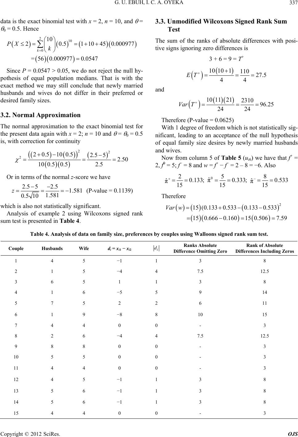

G. U. EBUH, I. C. A. OYEKA 337
data is the exact binomial test with x = 2, n = 10, and
 =

0 = 0.5. Hence
 
 
210
0
10
20.51 1045
= 560.0009770.0547
k
PX k


 





0.000977
Since P = 0.0547 > 0.05, we do not reject the null hy-
pothesis of equal population medians. That is with the
exact method we may still conclude that newly married
husbands and wives do not differ in their preferred or
desired family sizes.
3.2. Normal Approximation
The normal approximation to the exact binomial test for
the present data again with x = 2; n = 10 and  = 
0 = 0.5
is, with correction for continuity




2
220.5100.52.5
10 0.50.5



2
52.50
2.5

Or in terms of the normal z-score we have
2.55
1.
0.5 10
z 
2.5 1.581
581 

(P-value = 0.1139)
which is also not statistically significant.
Analysis of example 2 using Wilcoxons signed rank
sum test is presented in Table 4.
3.3. Unmodified Wilcoxons Signed Rank Sum
Test
The sum of the ranks of absolute differences with posi-
tive signs ignoring zero differences is
3 + 6 = 9 = T+


10 101110 27.5
44
ET



and




10 1121231096.25
24 24
Var T
Therefore (P-value = 0.0625)
With 1 degree of freedom which is not statistically sig-
nificant, leading to an acceptance of the null hypothesis
of equal family size desires by newly married husbands
and wives.
Now from column 5 of Table 5 (ui6) we have that f+ =
2, f0 = 5; f− = 8 and w = f+ − f− = 2 – 8 = −6. Also
0
258
ˆ
0.133;π0.333; 0.533
ˆˆ ππ
1515 15

  
  

2
15 (0.1330.5330.1330.533
150.6660.160150.5067.59
Var w 

Therefore
Table 4. Analysis of data on family size, preferences by couples using Walloons signed rank sum test.
i
d
Couple Husbands Wife di = xi1 − xi2 Ranks Absolute
Difference Omitting Zero
Rank of Absolute
Differences Including Zeros
1 4 5 −1 1 3 8
2 1 5 −4 4 7.5 12.5
3 6 5 1 1 3 8
4 1 6 −5 5 9 14
5 7 5 2 2 6 11
6 1 9 −8 8 10 15
7 4 4 0 0 - 3
8 2 6 −4 4 7.5 12.5
9 8 8 0 0 - 3
10 5 5 0 0 - 3
11 4 4 0 0 - 3
12 4 5 −1 1 3 8
13 5 6 −1 1 3 8
14 5 6 −1 1 3 8
15 4 4 0 0 - 3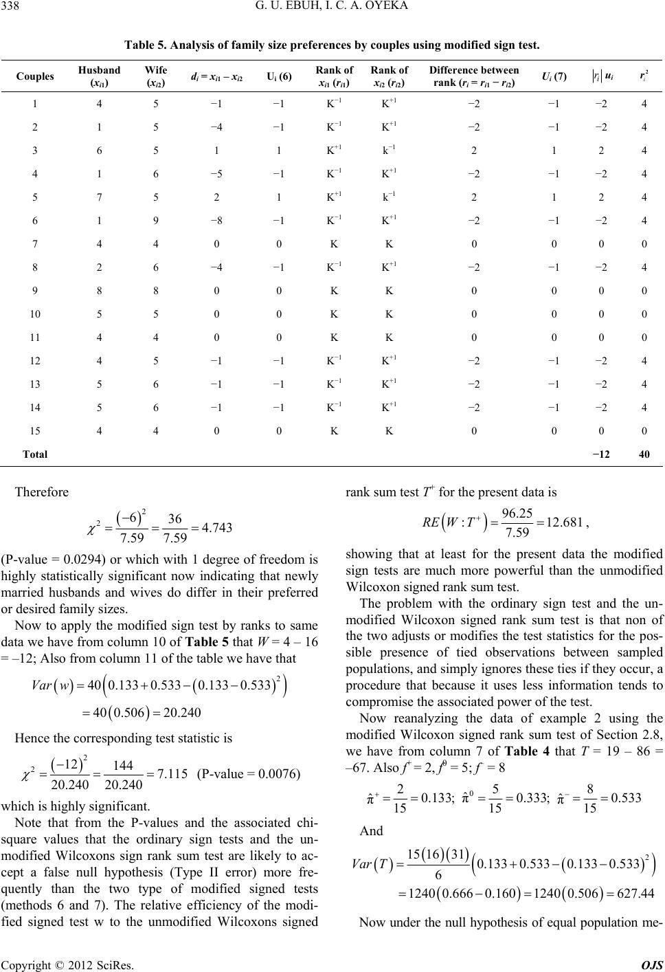

G. U. EBUH, I. C. A. OYEKA 338
Table 5. Analysis of family size preferences by couples using modified sign test.
Couples Husband
(xi1)
Wife
(xi2) di = xi1 – xi2 Ui (6) Rank of xi1 (ri1)
Rank of
xi2 (ri2)
Difference between
rank (ri = ri1 − ri2) Ui (7) i
ri
2
rui
1 4 5 −1 −1 K−1 K
+1 −2 −1 −2 4
2 1 5 −4 −1 K−1 K
+1 −2 −1 −2 4
3 6 5 1 1 K+1 k
−1 2 1 2 4
4 1 6 −5 −1 K−1 K
+1 −2 −1 −2 4
5 7 5 2 1 K+1 k
−1 2 1 2 4
6 1 9 −8 −1 K−1 K
+1 −2 −1 −2 4
7 4 4 0 0 K K 0 0 0 0
8 2 6 −4 −1 K−1 K
+1 −2 −1 −2 4
9 8 8 0 0 K K 0 0 0 0
10 5 5 0 0 K K 0 0 0 0
11 4 4 0 0 K K 0 0 0 0
12 4 5 −1 −1 K−1 K
+1 −2 −1 −2 4
13 5 6 −1 −1 K−1 K
+1 −2 −1 −2 4
14 5 6 −1 −1 K−1 K
+1 −2 −1 −2 4
15 4 4 0 0 K K 0 0 0 0
Total −12 40
Therefore

236 4.743
7.59 


2
.133 0.533
26
7.59



(P-value = 0.0294) or which with 1 degree of freedom is
highly statistically significant now indicating that newly
married husbands and wives do differ in their preferred
or desired family sizes.
Now to apply the modified sign test by ranks to same
data we have from column 10 of Table 5 that W = 4 – 16
= –12; Also from column 11 of the table we have that
 


40 0.1330.5330
40 0.50620.240
Var w 

Hence the corresponding test statistic is

21447.115
20.240


212
20.240


 (P-value = 0.0076)
which is highly significant.
Note that from the P-values and the associated chi-
square values that the ordinary sign tests and the un-
modified Wilcoxons sign rank sum test are likely to ac-
cept a false null hypothesis (Type II error) more fre-
quently than the two type of modified signed tests
(methods 6 and 7). The relative efficiency of the modi-
fied signed test w to the unmodified Wilcoxons signed
rank sum test T+ for the present data is
96.25
: 12.681
7.59
RE WT ,
showing that at least for the present data the modified
sign tests are much more powerful than the unmodified
Wilcoxon signed rank sum test.
The problem with the ordinary sign test and the un-
modified Wilcoxon signed rank sum test is that non of
the two adjusts or modifies the test statistics for the pos-
sible presence of tied observations between sampled
populations, and simply ignores these ties if they occur, a
procedure that because it uses less information tends to
compromise the associated power of the test.
Now reanalyzing the data of example 2 using the
modified Wilcoxon signed rank sum test of Section 2.8,
we have from column 7 of Table 4 that T = 19 – 86 =
–67. Also f+ = 2, f0 = 5; f– = 8
0
258
ˆ
0.133;π0.333; 0.533
ˆˆ
ππ
1515 15

  

And






2
15 16310.133 0.5330.133 0.533
6
1240 0.6660.1601240 0.506627.44
Var T

Now under the null hypothesis of equal population me-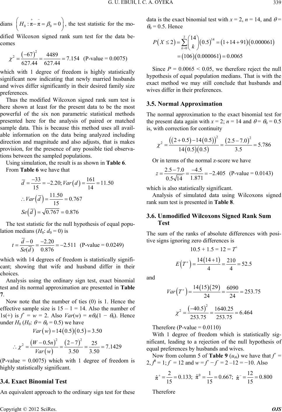

G. U. EBUH, I. C. A. OYEKA 339
dians , the test statistic for the mo-
00
ππ 0 





: H
dified Wilcoxon signed rank sum test for the data be-
comes

2
267
627.44 62



4489 7.154
7.44 
(P-value = 0.0075)
which with 1 degree of freedom is highly statistically
significant now indicating that newly married husbands
and wives differ significantly in their desired family size
preferences.
Thus the modified Wilcoxon signed rank sum test is
here shown at least for the present data to be the most
powerful of the six non parametric statistical methods
presented here for the analysis of paired or matched
sample data. This is because this method uses all avail-
able information on the data being analyzed including
direction and magnitude and also adjusts, that is makes
provision, for the presence of any possible tied observa-
tions between the sampled populations.
Using simulation, the result is as shown in Table 6.
From Table 6 we have that



33 2.20;
15
11.50 0.767
15
0.767 0.876
dV
Var d
Sed




161 11.50
14
ard 
The test statistic for the null hypothesis of equal popu-
lation medians (H0: d0 = 0) is
02
( )
d
tSed


.20
2.511
0.876 

(P-value = 0.0249)
which with 14 degrees of freedom is statistically signifi-
cant; showing that wife and husband differ in their
choices.
Analysis using the ordinary sign test, exact binomial
test and its normal approximation are presented in Table
7.
Now note that the number of ties (0) is 1. Hence the
effective sample size is 15 – 1 = 14. Also the number of
1s(+) is f+ = w = 2. Also Var(w) = n 
0(1 −

0). Hence
under H0 (H0:  = 
0 = 0.5) we have



0.5 3.5014 0.5Var w



22
20.52 7
3.50
Wn
Var w


 
25 7.1429
3.50 
 

214
0
14
20.5114910.000061
106 0.0000610.0065
k
PX k


 




 

(P-value = 0.0075) which with 1 degree of freedom is
highly statistically significant.
3.4. Exact Binomial Test
An equivalent approach to the ordinary sign test for these
data is the exact binomial test with x = 2, n = 14, and  =

0 = 0.5. Hence
Since P = 0.0065 < 0.05, we therefore reject the null
hypothesis of equal population medians. That is with the
exact method we may still conclude that husbands and
wives differ in their preferences.
3.5. Normal Approximation
The normal approximation to the exact binomial test for
the present data again with x = 2; n = 14 and  = 
0 = 0.5
is, with correction for continuity

22
220.514 0.52.5 7.05.786
14 0.50.53.5

 

Or in terms of the normal z-score we have
2.5 7.04.52.405
1.871
0.5 14
z




(P-value = 0.0143)
which is also statistically significant.
Analysis of simulated data using Wilcoxons signed
rank sum test is presented in Table 8.
3.6. Unmodified Wilcoxons Signed Rank Sum
Test
The sum of the ranks of absolute differences with posi-
tive signs ignoring zero differences is
10.5 + 1.5 = 12 = T+


14 14121052.5
44
ET



and




14 15296090 253.75
24 24
Var T

2
240.51640.25 6.464
253.75 253.75



Therefore (P-value = 0.0110)
With 1 degree of freedom which is statistically sig-
nificant, leading to a rejection of the null hypothesis of
equal preferences by husbands and wives.
Now from column 5 of Table 9 (ui6) we have that f+ =
2, f0 = 1; f− = 12 and w = f+ − f− = 2 –12 = −10. Also
0
2112
ˆ 0.133;π0.667; 0.800
ˆˆ
ππ
15 15 15


Therefore

G. U. EBUH, I. C. A. OYEKA 340
2
i
D
Table 6. Paired sample “t” test for the analysis of family size differences by a simulated random sample of husbands and wife
couples.
Couple Husband (xi1) Wife (xi2) Diff. di = xi1 – xi2
1 1 4 −3 9
2 7 8 −1 1
3 4 6 −2 4
4 4 6 −2 4
5 4 6 −2 4
6 8 4 4 16
7 2 6 −4 16
8 2 5 −3 9
9 2 8 −6 36
10 1 5 −4 16
11 5 9 −4 16
12 4 6 −2 4
13 4 9 −5 25
14 4 4 0 0
15 5 4 1 1
Total 5 − 38= −33 161
Table 7. Application of the ordinary sign test and other two to the simulated data on family size preferences by husbands and
wives.
Couple Husband (xi1) Wife (xi2) Diff. di = xi1 – xi2
2
i
u
1 1 4 −3 0
2 7 8 −1 0
3 4 6 −2 0
4 4 6 −2 0
5 4 6 −2 0
6 8 4 4 1
7 2 6 −4 0
8 2 5 −3 0
9 2 8 −6 0
10 1 5 −4 0
11 5 9 −4 0
12 4 6 −2 0
13 4 9 −5 0
14 4 4 0 -
15 5 4 1 1

G. U. EBUH, I. C. A. OYEKA 341
Table 8. Analysis of simulated data on family size, preferences by couples using Walloons signed rank sum test.
i
d
Couple Husbands Wife di = xi1 − xi2 Ranks Absolute
Difference Omitting Zero
Rank of Absolute
Differences including Zeros
1 1 4 −3 3 7.5 8.5
2 7 8 −1 1 1.5 2.5
3 4 6 −2 2 4.5 5.5
4 4 6 −2 2 4.5 5.5
5 4 6 −2 2 4.5 5.5
6 8 4 4 4 10.5 11.5
7 2 6 −4 4 10.5 11.5
8 2 5 −3 3 7.5 8.5
9 2 8 −6 6 14 15
10 1 5 −4 4 10.5 11.5
11 5 9 −4 4 10.5 11.5
12 4 6 −2 2 4.5 5.5
13 4 9 −5 5 13 14
14 4 4 0 0 - 1
15 5 4 1 1 1.5 2.5
Table 9. Analysis of simulated family size preferences by couples using modified sign test.
Couples Husb and
(xi1)
Wife
(xi2) di = xi1 – xi2 Ui (6) Rank of xi1 (ri1)
Rank of
xi2 (ri2)
Difference between
rank (ri = ri1 – ri2) Ui(7) i
ri
2
rui
1 1 4 −3 −1 K−1 K
+1 −2 −1 −2 4
2 7 8 −1 −1 K−1 K
+1 −2 −1 −2 4
3 4 6 −2 −1 K−1 K
+1 −2 −1 −2 4
4 4 6 −2 −1 K−1 K
+1 −2 −1 −2 4
5 4 6 −2 −1 K−1 K
+1 −2 −1 −2 4
6 8 4 4 1 K+1 K
−1 2 1 2 4
7 2 6 −4 −1 K−1 K
+1 −2 −1 −2 4
8 2 5 −3 −1 K−1 K
+1 −2 −1 −2 4
9 2 8 −6 −1 K−1 K
+1 −2 −1 −2 4
10 1 5 −4 −1 K−1 K
+1 −2 −1 −2 4
11 5 9 −4 −1 K−1 K
+1 −2 −1 −2 4
12 4 6 −2 −1 K−1 K
+1 −2 −1 −2 4
13 4 9 −5 −1 K−1 K
+1 −2 −1 −2 4
14 4 4 0 0 K K 0 0 0 0
15 5 4 1 1 K+1 K
−1 2 1 2 4
Total −20 56

G. U. EBUH, I. C. A. OYEKA
12 SciRes. OJS
342


2
800
81 7.3215


Now under the null hypothesis of equal population me-
 
 
15(0.1330.8000.1330.
150.9330.4449150.48
Var w 

Copyright © 20
Therefore

2
210 10
7.95 7.321



013.6584
5


2
0.800
1 27.334


(P-value = 0.00020)
or which with 1 degree of freedom is statistically signifi-
cant now indicating that husbands and wives preferences
differs.
Now to apply the modified sign test by ranks to same
data we have from column 10 of Table 9 that W = 4 – 24
= –20; Also from column 11 of the table we have that
 
 
56 (0.1330.8000.133
560.9330.444956 0.488
Var w 

Hence the corresponding test statistic is

2
220
27.334 27.33



400 14.634
4
(P-value = 0.00010)
which is highly statistically significant.
Note that from the P-values and the associated chi-
square values that the ordinary sign test and unmodified
wilcoxon sign rank sum test have lower P-values than the
two type of modified signed tests (methods 6 and 7). The
relative efficiency of the modified signed test w to the
unmodified Wilcoxons signed rank sum test T+ for the
simulated data is

25
:=27 RE WT3.759.283
.334 ,
showing that also for the simulated data the modified
sign tests are much more powerful than the unmodified
Wilcoxon signed rank sum test.
The problem with the ordinary sign test and the un-
modified Wilcoxon signed rank sum test is that non of
the two adjusts or modifies the test statistics for the pos-
sible presence of tied observations between sampled
populations, and simply ignores these ties if they occur, a
procedure that because it uses less information tends to
compromise the associated power of the test.
Now reanalyzing the simulated data using the modi-
fied Wilcoxon signed rank sum test of Section 2.8, we
have from column 7 of Table 8 that T = 14 –105 = –91.
Also f+ = 2, f0 = 1; f − = 12
0
21
ˆ
0.133;π0.667;
ˆˆ π
15 15

 12
0.800
π
15


and
  


2
3 0.800
881

00
:ππ 0H 




15 16310.133 0.8000.13
6
1240 0.9330.44491240 0.4
605.244
Var T


dians





, the test statistic for the mo-
dified Wilcoxon signed rank sum test for the data be-
comes
2
291 8281 13.682
605.244 605.244


 (P-value = 0.00019)
which with 1 degree of freedom is highly statistically
significant now indicating that couples differ signifi-
cantly in their preferences.
Thus the modified Wilcoxon signed rank sum test is
here shown again to be the second best using the simu-
lated data being the second most powerful of the six non
parametric statistical methods presented here for the
analysis of paired or matched sample data. This is be-
cause this method uses all available information on the
data being analyzed including direction and magnitude
and also adjusts, that is makes provision, for the presence
of any possible tied observations between the sampled
populations.
4. Summary and Conclusion
We have in this paper presented and discussed eight al-
ternative methods for the analysis of paired or matched
sample data. If the sampled populations satisfy the nec-
essary assumptions of continuity and normality, then the
paired sample parametric “t” test becomes the method of
choice and should be preferred since it is generally more
powerful than most alternative non parametric methods.
If however the data being analyzed are not continuous or
are ordinal non-numeric measurements, then the modi-
fied sign tests using either the raw scores themselves
(method 6) or their ranks (method 7) are the only avail-
able methods of analysis under the circumstance. If the
data are numeric measurements on at least the ordinal
scale but not appropriate for analysis using the paramet-
ric “t” test, then the modified Wilcoxon signed rank sum
test, the modified sign tests by ranks, the modified sign
test, the exact binomial or ordinary sign test and its nor-
mal approximation should be preferred and used in this
order because of their relatively decreasing power, as
shown by at least the illustrative examples used here and
when reanalyzed using simulation, the modified sign test
by ranks, modified Wilcoxon signed rank sum test, the
modified sign test, the exact binomial or its ordinary sign
test should be preferred and used in this order because of
their relative decreasing power which is almost the same
with the raw example except that modified sign tests by
rank came first using simulation while second using raw
data.
Finally each of the proposed methods may be appro-
priately modified and used to analyse one sample data

G. U. EBUH, I. C. A. OYEKA 343
simply by setting values or scores from one of the sam-
pled populations equal to some hypothesized value of a
measure of central tendency.
REFERENCES
[1] I. C. A. Oyeka, “An Introduction to Applied Statistical
Methods,” 8th Edition, Nobern Avocation Publishing
Company, Enugu, 2009.
[2] S. Siegel, “Non-Parametric Statistics for the Behavioral
Sciences,” McGraw-Hill Series in Psychology, New York,
1956.
[3] J D. Gibbons, “Non-Parametric Statistical Inference,”
McGraw Hill, New York, 1971.
[4] I. C. A. Oyeka, C. E. Utazi, C. R. Nwosu, P. A. Ikpegbu,
G. U. Ebuh, H. O. Ilouno and C. C. Nwankwo, “Method
of Analysing Paired Data Intrinsically Adjusted for Ties,”
Global Journal of Mathematics, Vol. 1, No. 1, 2009, pp.
1-6.
[5] I. C. A. Oyeka and G. U. Ebuh, “Modified Wilcoxon
Signed Rank Sum Test,” Open Journal of Statistics, Vol.
2, No. 2, 2012, pp. 172-176. doi:10.4236/ojs.2012.22019

G. U. EBUH, I. C. A. OYEKA 344
Appendix 1: A Summary of Eight Alternative Test Statistics for the Analysis of
Paired Samples
S/N Method Statistic Variance
(under H0)
Test Statistic
(under H0) Assumption Comments
1 Parametric
Test
d (mean of
sample
difference)
2d
s
0
tdd


n
s
n
Populations
continuous and
normally
distributed;
measurements
on the ratio scale
Most powerful if
necessary
assumptions
are satisfied.
2 Ordinary
Sign Test
W(=No. of 1’s
or −1’s) n

0(1 −

0)


2
20
00
1
wn
n






Population
continuous
numeric
measurements
on at least the
ordinary scale
Usually ignores
tied observations
uses effective
sample size (total
number of
non-zero
differences).
3 Exact
Binomial Test
W = X’ = x
(=No.
of 1’s or −1’s)

2
0k
Px

00
21
nk
k
n
k




  

Population
numeric and
discrete
4
Normal
Approximation
to the Sign Test
W(=No. of 1’s
or −1’s)

00
1n

 





0
00
0.5
1
wn
n
t





Population
discrete “n”
sufficiently large
Incorporates
continuity
correction.
5
Unmodified
Wilcoxon
Signed Rank
Sum Test
T+ = (sum of
the ranks of
absolute
differences
with
positives sign).


12
6
1
nn
 

1n

2
0
00
1
11
6
n

2
2
12
u
nn
T
nn





 



Population
continuous
numeric
measurement
on at least the
ordinal scale
Ignores zero
absolute
differences;
does not provide
for tied
observations
between samples.
6 Modified
Sign Test
W = (difference
between total
number of
1s and −1s


2
ˆˆ ˆˆ
ππ ππn   





2
2
2
ˆˆ
ππ
ˆˆ ˆˆ
ππ ππ
wn
n


 

 
Population may
be non numeric
measurement on
at least the
ordinal scale
May be used with
both numeric and
non numeric
measurements on
at least the
ordinal scale.
Intrinsically
adjusted for any
possible tied
observations
between sampled
population more
powerful than the
unmodified
Wilcoxon signed
rank sum test.
7 Modified Sign
Test by Ranks W = R.1 – R.2





2
21nk t





.1 .2
2
2
ˆˆˆˆ ππ ππ
=4
ˆˆˆˆ ππ ππ
nt
 
 
 

 
 



22
rr 2




2
2
22 2
.1 .2
2
2
ˆˆ ˆˆ 21ππππ
=
ˆˆˆˆ
4ππππ
w
rr nkt
w
nt
 
 
 

Population may
be non numeric
measurement
on at least the
ordinal scale
Same as No. 6
except that if uses
the ranks of the
paired
observations
rather than the
observations
themselves; may
be used for
numeric and non
numeric
measurements on
at least the
ordinal scale,
intrinsically
adjusted for ties,
also more
powerful than the
unmodified
Wilcoxon Signed
Rank Sum Test.

G. U. EBUH, I. C. A. OYEKA 345
Continued
8
Modified
Wilcoxon
Signed Rank
Sum Test
T (=difference
between the
sum of ranks o
f
absolute
differences
with positive
signs and the
sum of the
ranks of
absolute
differences
with negative
signs)
 


2
6
ππ ππ
nn
 
 

12 1n

 

2
2
2
1.ππ
2
121 ˆˆˆˆ
ππ ππ
6
nn
T
nn n


 


 



Population
numeric
measurement
on at least the
ordinal scale
Intrinsically
adjusted for any
possible tied
observations
between sampled
populations, if
applicable is the
most powerful of
all the
non-parametric
tests presented
here.