Journal of Environmental Protection, 2010, 1, 172-178
doi:10.4236/jep.2010.12021 Published Online June 2010 (http://www.SciRP.org/journal/jep)
1
Comparison between Non-Gaussian Puff Model and a Model
Based on a Time-Dependent Solution of Advection-Diffusion
Equation
Tiziano Tirabassi1, Davidson M. Moreira2, Marco Tullio Vilhena3, Camila Pinto da Costa4
1Institute of Atmospheric Sciences and Climate (ISAC), National Research Council (CNR), Bologna, Italy; 2Federal University of
Pampa (UNIPAMPA), Bagé, Brazil; 3Federal University of Rio Grande do Sul (UFRGS), Porto Alegre, Brazil; 4Federal University
of Pelotas (UFPel), Pelotas, Brazil.
Received March 30th, 2010; revised April 27th, 2010; accepted April 29th, 2010.
ABSTRACT
A comparison between a non-Gaussian puff model and an advanced time-dependent model to simulate the pollutant
dispersion in the Planetary Boundary Layer is presented. The puff model is based on a general technique for solving the
K-equation, using the truncated Gram-Charlier expansion (type A) of the concentration field and finite set equations for
the corresponding moments. The other model (named ADMM: Analytical Dispersion Multilayers Model) is an semi-
analytical solution to the time-dependent two-dimensional advection-diffusion equation based on a discretization of the
PBL in N sub-layers; in each sub-layers the advection-diffusion equation is solved by the Laplace transform technique,
considering an average value for eddy diffusivity and the wind speed. A preliminary performance evaluation is shown
in the case of continuous emission from an elevated source in a variable boundary layer. Both models were able to
correctly reproduce the concentration field measured and so to be used as operative air pollution models.
Keywords: Advection-Diffusion Equation, Air Pollution Modeling, Analytical Solution, Puff Models
1. Introduction
Both our scientific understanding and technical devel-
opments have been greatly increased by the use of em-
pirical, analytical and numerical models to predict the air
pollution concentration in atmosphere. For this purpose,
the advection-diffusion equation has been largely applied
in operational atmospheric dispersion models. In princi-
ple, from this equation it is possible to obtain the disper-
sion from a source given appropriate boundary and initial
conditions plus knowledge of the mean wind velocity
and concentration turbulent fluxes [1].
Gaussian models are theoretically based upon an exact,
but not realistic solution of the equation of transport and
diffusion in the atmosphere, in cases where both wind
and turbulent diffusion coefficients are constant with
height. The solution is forced to represent real situations
by means of empirical parameters, referred to as “sig-
mas”. They can be either stationary (the plume models)
or time-dependent (puff models).
Quasi-instantaneous and short-term releases are fre-
quently viewed as “puff” releases. A puff release sce-
nario assumes that the release time and sampling times
are very short compared to the travel time from the
source to the receptor.
The various versions of Gaussian models essentially
differ in the techniques utilized to calculate the sigmas as
a function of atmospheric stability and the downwind
distance from the emission source [2]. Gaussian models
are fast, simple and do not require complex meteorologi-
cal inputs (in comparison to numerical models). For these
reasons they are still widely used by the environmental
agencies all over the world for regulatory applications.
Nonetheless, because of their well known intrinsic
limits, the reliability of a Gaussian model strongly de-
pends on the way the dispersion parameters are deter-
mined on the basis of the turbulence structure of the
planetary boundary layer (PBL) and the model’s ability
to reproduce experimental diffusion data. A great variety
of formulations exist [3-10]. One of the most popular
Gaussian models is AERMOD [11] and among puff
models CALPUFF [12] has to be outlined.
Among non-Gaussian models we outline the puff
model proposed by van Ulden [13], the plume non-

Comparison between Non-Gaussian Puff Model and a Model Based on a Time-Dependent 173
Solution of Advection-Diffusion Equation
Gaussian model by Sharan and Modani [14] and analyti-
cal models presented in [15].
In order to take in account the puff releases, Reference
[16] developed a K-model for the dispersion of passive
non-Gaussian puffs. The model is based on a general
technique for solving the advection-diffusion equation
using the truncated Gram-Charlier expansion of the con-
centration field and the finite set of equations for the
corresponding moments. Actually, the Gram-Charlier
expansion of type A is a classical method for approxi-
mating a given distribution with moments of any order,
basically consisting of a truncated expansion in terms of
Hermite functions, whose coefficients are chosen so as to
reproduce the sequence of moments of the distribution up
to a given order [17].
Moreover, recently was obtained a semi-analytical
solution of the advection-diffusion equation for non-
stationary conditions [18]. From this solution a model
named ADMM has been set up. The model is based on a
discretization of the PBL in N sub-layers, where in each
sub-layers the advection-diffusion equation is solved by
the Laplace transform technique, considering an average
value for eddy diffusivity and the wind speed. The main
feature of this method relies on the following steps:
stepwise approximation of the eddy diffusivity and wind
speed, double Laplace transform application to the ad-
vection-diffusion equation in the x and t variable,
semi-analytical solution of the set of linear ordinary
equation resulting for the double Laplace transform ap-
plication and construction of the pollutant concentration
by the Laplace transform inversion using the Gaussian
quadrature scheme (semi-analytical due to the numeric
inversion).
The main objective of this paper is to present and dis-
cuss the results of a comparison between the non-
Gaussian puff, where the concentration field is approxi-
mated because only the first four moments of the con-
centration distribution is used, and an advanced time de-
pendent model, that accept general profiles for wind and
eddy diffusivity coefficients (as well as the theoretical
profiles proposed in the scientific literature, such as the
vertical profiles of eddy diffusion coefficients predicted
by the Similarity Theory), but they are described by a
stepwise function.
2. The Models
2.1 The Puff Model
The advection diffusion equation describing the time
evolution of concentration C, due to a release at time
of a quantity Q of passive material by an elevated
source placed at (0,0,1), in a horizontally homogeneous
atmospheric boundary layer is:
0t
22
22 2
1() () ( ) (1)
z
h
CC CC
udv K
txyz z
CC
Ktx
dx y
 
 

 

 


 yz

 




(1)
where x is the along-wind coordinate, y the crosswind
one and z the height;

means delta function, (u,v,0) is
the wind velocity vector, z
K
and are the eddy
diffusivities for vertical and horizontal turbulent trans-
port, respectively. In this chapter all variables are
non-dimensional, the corresponding scale factors being
given by
h
K
ss KH 2 for time, for a dis-
tance along the x-axis, for the height and distance
along the y axis, for diffusivities, for wind
speed and
ss dHKH /
2
s
u
s s
U
s
H
s
K
3
0()
s
QdH for concentration. and
represent the values of the dimensional u and K profiles
at the dimensional source .
s
Ks u
s
H
The initial condition is:
0
lim C(x,y,z,t)0
t  (2)
And the no-flux boundary conditions applied at the
ground level and at the mixing layer height () are:
i
z
0
z
C
Kz


 for 0z

and (3)
i
zz
Since C is exponentially small at asymptotic distances
from the source on any horizontal plane, we can intro-
duce the moments of its (x,y)-distribution:
,
mn
mn
CxyCd
 
 
 xdy
(4)
where m, n are non-negative integers.
Of course, are functions of height and time.
Their time evolution is governed by the double sequence
of 1-dimensional diffusion equations, equivalent to the
single three-dimensional (1):
,mn
C

0,0
0,0
,
,1,,1
2
2,, 2
() (1)
1/(1)( 1)
mn
mnm nmn
hmn
CDCtz
t
CDCmuCn dv C
t
KdmmC nnC


 mn

 

 


(5)
For 0mn

and D the differential operator




/
z
zK Cz/

.
The initial condition is therefore written:
+
0
lim =0
m,n
t
C
 (6)
And the boundary conditions becomes:

Comparison between Non-Gaussian Puff Model and a Model Based on a Time-Dependent
174
Solution of Advection-Diffusion Equation
0
z
C
Kz

 at (7) 0, i
zz
A classic method for approximating a given distribu-
tion with moments of any order is the Gram-Chalier ex-
pansion of type A, which is basically constituted by a
truncated expansion in terms of Hermite functions,
whose coefficients are chosen so as to reproduce the se-
quence of moments of the function up to a given order
[19].
In the case of one-variate function of the concentration
, truncated to the fourth order, if is the skew-
ness and is the Kurtosis, we have [16]:
)(xC k S
u
K

2/2
0
42 2
2
3
163
24 6
uk
e
CC
KS


 




 




3


(8)
where:
x
b




1
0
C
bC 
22
2
0
Cb
C
 
23
3
30
13
k
C
Sb
C






b
223 4 4
40
164
u
C
KbbS
C






k
b



2.2 ADMM Model
A typical problem in air pollution studies is to seek the
solution for the cross-wind (y direction) integrated con-
centration for a continuous source of pollution (being
lateral concentration distribution usually assumed Gaus-
sian), that is:
z
CC C
uK
txz z








(9)
where C is the dimensional cross-wind integrated con-
centration (from this section all the variable are dimen-
sional).
The mathematical description of the dispersion prob-
lem represented by the (9) is well posed when it is pro-
vided by initial and boundary conditions. Indeed, it is
assumed that at the beginning of the contaminant release
the dispersion region is not polluted, this means:
(,,0)0Cxz at t = 0 (10)
At the point (0,, )
s
H
t a continuous line source of the
constant emission rate Q is assumed
0,( )
s
Q
C(,z t)=zH
u
  at x = 0 (11)
where δ is the Dirac delta function and Hs the source
height.
The pollutants are also subjected to the boundary con-
ditions of zero flux at ground and PBL top:
0
z
C
Kz



at (12) 0, i zz
where is the vertical depth of mixing region (PBL
height).
i
z
Bearing in mind the dependence of the Kz coefficient
and wind speed profile u on variable z, the height of
a PBL is discretized in N sub-intervals in such a manner
that inside each interval Kz and u assume the average
value:
i
z
1
1
1()
n
n
z
n
nn
z
z
K
Kzdz
zz


 (13)
1
1
1()
n
n
z
n
nn
z
u
zz


uzdz (14)
Therefore the solution of (9) is reduced to the solution
of N problems of the type:
2
2
nn n
nn
CC C
uK
tx z





1n zzz
n

 (15)
for n = 1,…,N – 1, where n
CC denotes the concen-
tration at the nth sub-interval. To determine the 2N inte-
gration constants the additional (2N – 2) condition
namely continuity of concentration and flux at interface
are considered:
1nn
CC

 n = 1, 2,...(N – 1) (16)
1
1
n
nn
CC
KK
zz
n





 n = 1, 2,...(N – 1) (17)
Applying the Laplace transform in (15) results:
2
2
()
(, ,)(, ,)(0, ,)
nn
nn
nn
psu u
CszpC szpCzp
KK
zn




(18)
where


(, ,)(, ,);;
nn
Cszp LCxztxstp, which
has the well-know solution:

((
(, ,)
2
nn
ns ns
Rz Rz
nnn
RzHRzH
a
Cszp AeBe
Qee
R

 


)
(19)
where

Comparison between Non-Gaussian Puff Model and a Model Based on a Time-Dependent 175
Solution of Advection-Diffusion Equation
(
n
n
n
psu
RK

)
and ()
an
RpsuK n
Finally, applying the initial and boundary conditions
we get a linear system for the integration constants.
Henceforth the concentration is obtained by inverting
numerically the transformed concentration n
C by Gaus-
sian quadrature scheme [18]:
11
()
()
()
(,,)
1()
2
jn jn
ii
s
nn nn
jn
i
s
nn
jn
i
s
nn
kM
j
i
ij
iJ
Pu Pu
PP
zH
tK xKtK xK
nn
Pu
P
zH tK xK
s
Pu
P
jn
izHtKxK
n
P
P
Cxzt ww
tx
Ae Be
e
QHz H
Pu
PK
tx e

 
 
 
 
 


 











 















 
















(20)
where

s
H
zH
i
P
is the Heaviside function that multi-
plies the part of (20) that is different from 0 only in the
sublayer that contains the source. The values of ,
(weights) and , (roots) of the Gaussian quadrature
scheme are tabulated in the book by Stroud and Secrest
[20] and k and m are the quadrature points.
i
wj w
j
P
The semi-analytical character of the solution (20) re-
duces to the solution of [21] when the time goes to infin-
ity (
t
). For more details see [22-24].
3. Boundary Layer Parameterization
We applied a parameterization proposed by Troen and
Marth [25], as presented in Pleim and Chang [26]. Dur-
ing near neutral and stable conditions (10
i
zL ), we
adopted:
2
*(1/ )
(/ )
i
z
h
ku zzz
KzL

 (21)
where

12
116
hzL
 .
During convective conditions (10Lzi) the friction
velocity was replaced by the convective velocity () as
scaling velocity, to give [26]:
*
w
*(1/) zi
K
kw zzz (22)
where k is the von Karman constant (k~0.4).
For the horizontal eddy diffusivity in unstable condi-
tions (in the puff model), we use [27]:
*
0.1
h
In neutral-stable conditions [28]:
2
hMz
K
K

(24)
where
M
z
K
is the maximum ofz
K
.
4. Validation against Experimental Data
For a better understanding of the comparison between the
two models in this work, we focus our attention on the
mathematical features of the two approaches. Concerning
the semi-analytical method it is relevant to underline that
in this approach no approximation is made in its deriva-
tion except for the stepwise approximation of the mete-
orological parameters and the Laplace numerical inver-
sion by the Gaussian quadrature scheme. It is well known,
that the results attained by the Gaussian quadrature
scheme of order N, are exact when the transformed func-
tion is a polynomial of degree (2N – 1). It is possible,
performing relative error calculation, between numerical
results with k + 1 and k points of quadrature as well for
m + 1 and m points, to control the error in the Gaussian
quadrature scheme, by properly choosing k and m, in
order to attain a prescribed accuracy. Concerning the
issue of stepwise approximation, it is important to bear in
mind that the stepwise approximation of a continuous
function converges to the continuous function, when the
stepwise of the approximation goes to zero. For the
semi-analytical method it is only necessary to choose the
number of the sub-layers in an appropriate manner, by
taking the smoothness of the functions and into
account.
z
Ku
On the other hand regarding the puff model, deriva-
tives of the resulting system of equations are approxi-
mated by a finite difference scheme, which does not oc-
cur in the semi-analytical method. According to the Lax
equivalence theorem [29] for linear autonomous prob-
lems, the convergence of the numerical schemes de-
mands the fulfillment of the requirements of stability and
consistency. In order to achieve the stability conditions,
the numerical methods like the one considered in this
work, impose a large number of step calculations used in
performing the time integration for all times. This feature
does not appear in the semi-analytical method, because
the semi-analytical character of the solution allows us to
perform the calculation at any time. This guarantees the
smaller computational time as well the smaller round-off
error influence in the accuracy of the results of the
semi-analytical method when compared with the nu-
merical ones, because it demands less mathematical op-
erations. Moreover the concentration field is described
only using the first four moments of the concentration
distribution. In fact we use the Gram-Charlier expansion
(type A) of the concentration field truncated at the fourth
moment.
i
K
wz (23) A preliminary evaluation of the performances of the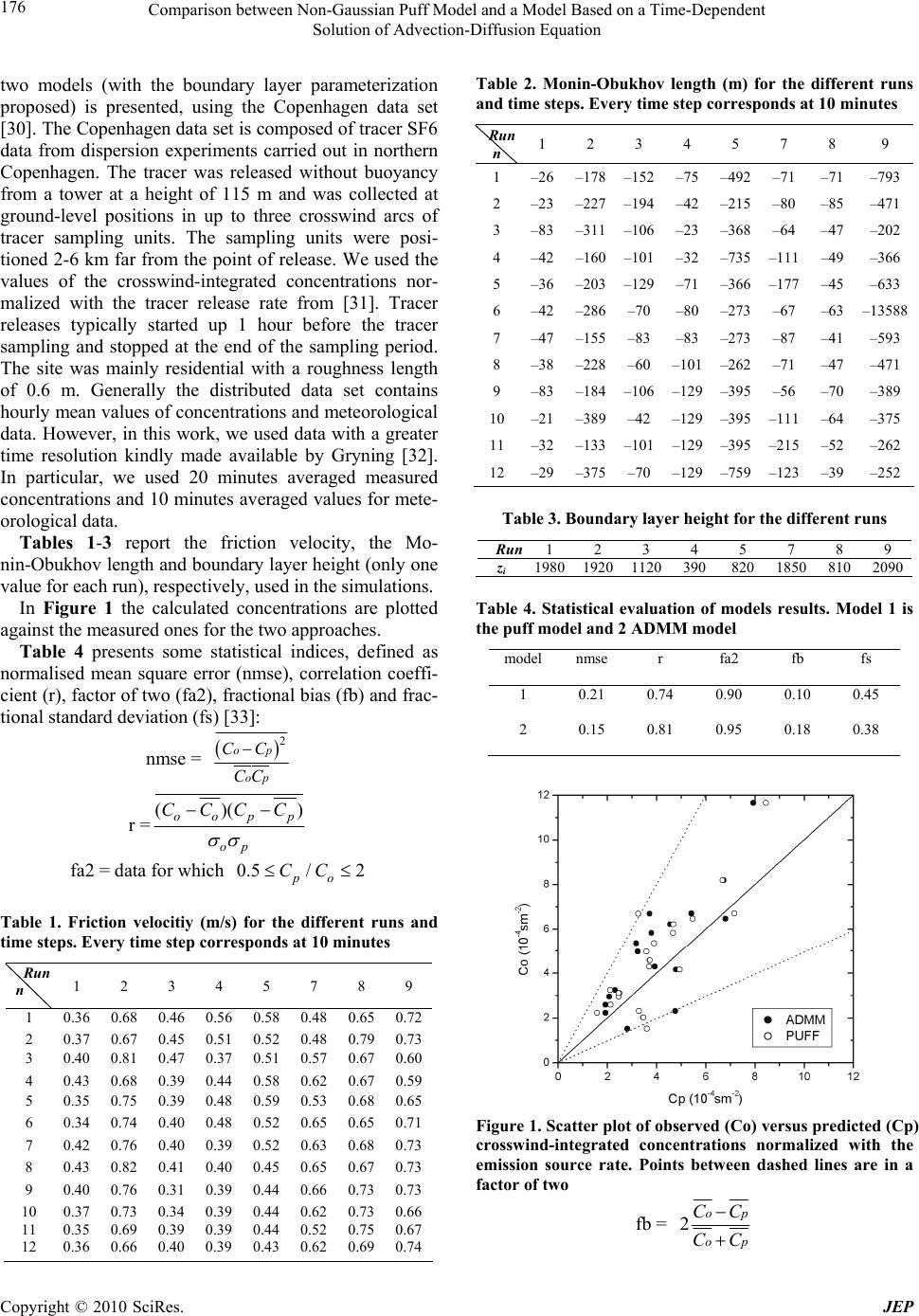

Comparison between Non-Gaussian Puff Model and a Model Based on a Time-Dependent
176
Solution of Advection-Diffusion Equation
two models (with the boundary layer parameterization
proposed) is presented, using the Copenhagen data set
[30]. The Copenhagen data set is composed of tracer SF6
data from dispersion experiments carried out in northern
Copenhagen. The tracer was released without buoyancy
from a tower at a height of 115 m and was collected at
ground-level positions in up to three crosswind arcs of
tracer sampling units. The sampling units were posi-
tioned 2-6 km far from the point of release. We used the
values of the crosswind-integrated concentrations nor-
malized with the tracer release rate from [31]. Tracer
releases typically started up 1 hour before the tracer
sampling and stopped at the end of the sampling period.
The site was mainly residential with a roughness length
of 0.6 m. Generally the distributed data set contains
hourly mean values of concentrations and meteorological
data. However, in this work, we used data with a greater
time resolution kindly made available by Gryning [32].
In particular, we used 20 minutes averaged measured
concentrations and 10 minutes averaged values for mete-
orological data.
Tables 1-3 report the friction velocity, the Mo-
nin-Obukhov length and boundary layer height (only one
value for each run), respectively, used in the simulations.
In Figure 1 the calculated concentrations are plotted
against the measured ones for the two approaches.
Table 4 presents some statistical indices, defined as
normalised mean square error (nmse), correlation coeffi-
cient (r), factor of two (fa2), fractional bias (fb) and frac-
tional standard deviation (fs) [33]:
nmse =

2
op
op
CC
CC

r = ()(
oop p
op
CCCC

)
fa2 = data for which 0.5/ 2
po
CC
Table 1. Friction velocitiy (m/s) for the different runs and
time steps. Every time step corresponds at 10 minutes
R
un
n 1 2 3 4 5 7 8 9
1 0.36 0.68 0.46 0.560.58 0.48 0.650.72
2 0.37 0.67 0.45 0.510.52 0.48 0.790.73
3 0.40 0.81 0.47 0.370.51 0.57 0.670.60
4 0.43 0.68 0.39 0.440.58 0.62 0.670.59
5 0.35 0.75 0.39 0.480.59 0.53 0.680.65
6 0.34 0.74 0.40 0.480.52 0.65 0.650.71
7 0.42 0.76 0.40 0.390.52 0.63 0.680.73
8 0.43 0.82 0.41 0.400.45 0.65 0.670.73
9 0.40 0.76 0.31 0.390.44 0.66 0.730.73
10 0.37 0.73 0.34 0.390.44 0.62 0.730.66
11 0.35 0.69 0.39 0.390.44 0.52 0.750.67
12 0.36 0.66 0.40 0.390.43 0.62 0.690.74
Table 2. Monin-Obukhov length (m) for the different runs
and time steps. Every time step corresponds at 10 minutes
R
un
n 1 2 3 4 5 7 8 9
1 –26–178–152–75 –492 –71 –71–793
2 –23–227–194–42 –215 –80 –85–471
3 –83–311–106–23 –368 –64 –47–202
4 –42–160–101–32 –735 –111 –49–366
5 –36–203–129–71 –366 –177 –45–633
6 –42–286–70–80 –273 –67 –63–13588
7 –47–155–83–83 –273 –87 –41–593
8 –38–228–60–101 –262 –71 –47–471
9 –83–184–106–129 –395 –56 –70–389
10–21–389–42–129 –395 –111 –64–375
11–32–133–101–129 –395 –215 –52–262
12–29–375–70–129 –759 –123 –39–252
Table 3. Boundary layer height for the different runs
R
un 1 2 3 4 5 7 8 9
zi 198019201120390 820 1850 8102090
Table 4. Statistical evaluation of models results. Model 1 is
the puff model and 2 ADMM model
model nmse r fa2 fb fs
1 0.21 0.74 0.90 0.10 0.45
2 0.15 0.81 0.95 0.18 0.38
Figure 1. Scatter plot of observed (Co) versus predicted (Cp)
crosswind-integrated concentrations normalized with the
emission source rate. Points between dashed lines are in a
factor of two
fb = 2op
op
CC
CC



Comparison between Non-Gaussian Puff Model and a Model Based on a Time-Dependent 177
Solution of Advection-Diffusion Equation
fs = 2op
op



 

where the subscript “o” and “p” are for the observed and
predicted concentrations, respectively, while

is the
standard deviation.
Analysing the statistical indices in Table 4 it is possi-
ble to notice that the models simulate satisfactorily the
observed concentrations, with nmse, fb and fs values
relatively near to zero and r and fa2 relatively near to 1.
A more detailed inspection of the Table 4 permits to ob-
serve that ADMM presents best values of nmse, r and fa2
while the puff model presents best values of fb.
5. Conclusions
The aim of this paper was to present and discuss the re-
sults of a comparison between non-Gaussian puff model
and a model based on a time-dependent semy-analytical
solution of advection-diffusion equation to simulate pol-
lutant dispersion in the PBL, focusing the ability to cor-
rectly reproduce the concentration field measured during
the Copenhagen tracer experiments, considering the me-
teorological parameters varying with time.
Models performances were evaluated using data from
the Copenhagen data set, but with a time resolution
greater than the data ones generally distributed [34], pre-
senting good results for both approaches. In particular,
we used 20 minutes average concentrations of SF6 and
10 minutes average values for meteorological data.
The two models present comparable results and, in this
preliminary evaluation, their performance does not show
any correlation with the meteorological characterization
of the PBL. Both models underestimate the ground level
concentrations, probably due to the turbulence parame-
terization used.
6. Acknowledgements
The authors are gratefully indebted to CNPq, FAPERGS,
CNR and ENVIREN for the partial financial support of
this work.
REFERENCES
[1] S. P. Arya, “Air Pollution Meteorology and Dispersion,”
Oxford University Press, Oxford, 1999, p. 310.
[2] P. Zannetti, “Air Quality Modeling III,” The EnvironComp
Institute and Air & Waste Management Association,
Fremont, 2008, p. 485.
[3] S. R. Hanna, G. A. Briggs, J. Deardoff, B. A. Egan, F. A.
Gifford and F. Pasquill, “AMS Workshop on Stability
Classification Schemes and Sigmas Curves—Summary of
Recommendations,” Bulletin of the American Meteorological
Society, Vol. 58, No. 12, 1977, pp. 1305-1309.
[4] G. A. Briggs, “Plume Rise Predictions,” Lectures on Air
Pollution and Environmental Impact Analyses, Workshop
Proceedings, American Meteorological Society, Boston,
29 September-3 October 1975, pp. 59-111.
[5] S. R. Hanna, “Lateral Dispersion from Tall Stacks,” Journal
of Climmate Applied Meteorology, Vol. 25, No. 10, 1986,
pp. 1426-1433.
[6] R. Berkowicz, H. R. Olesen and U. Torp, “The Danish
Gaussian Air Pollution Model (OML): Description, Test
and Sensivity Analysis in View of Regulatory Applications,”
In: C. De Wispelaere, F. A. Schiermeier and N. V. Gillani,
Eds., Proceedings of NATO-CCMS 16th International
Meeting on Air Pollution, Modelling and its Applications,
Plenum Press, New York, 1986, pp. 453-481.
[7] B. M. Bowen, “Long-Term Tracer Study at Los Alamos,
New Messico. Part II: Evaluation and Comparison of
Several Methods to Determinate Dispersion Coefficients,”
Journal of Appied Meteorology, Vol. 33, No. 11, 1994, pp.
1236-1254.
[8] J. J. Erbrink, “Use of Boundary-Layer Meteorological
Parameters in the Gaussian Model ‘Stacks’,” Bounary-
Layer Meteorology, Vol. 74, No. 3, 1995, pp. 211-235.
[9] M. Mohan and T. A. Siddiqui, “An Evaluation of Dispersion
Coefficients for Use in Air Quality Models,” Bounary-
Layer Meteorology, Vol. 84, No. 2, 1997, pp. 177-205.
[10] B. J. Tsuang, “Quantification on the Source/Receptor
Relationship of Primari Pollutants and Secondary Aerosols
by a Gaussian Plume Trajectory Model: Part I – Theory,”
Atmospheric Environment, Vol. 37, No. 28, 2003, pp. 3981-
3991.
[11] A. J. Cimorelli, S. G. Perry, A. Venkatram, J. C. Weil, R.
J. Paine, R. B. Wilson, R. F. Lee, W. D. Peters and R. W.
Brode, “AERMOD: A Dispersion Model for Industrial
Source Applications. Part I: General Model Formulation
and Boundary Layer Characterization,” Journal of Appied
Meteorology, Vol. 44, No. 5, 2005, pp. 682-693.
[12] J. S. Scire, D. G. Strimaitis and R. J. Yamartino, “A
User’s Guide for the CALPUFF Dispersion Model,”
Version 5, Earth Tech Inc., Lowell, 2000. http://www.src.
com/calpuff/calpuff1.htm
[13] A. P. van Ulden, “A Surface-Layer Similarity Model for
the Dispersion of a Skewed Passive Puff near the Ground,”
Atmospheric Environment, Vol. 26, No. 4, 1992, pp. 681-
692.
[14] M. Sharan and M. Modani, “A Two-Dimensional Ana-
lytical Model for the Dispersion of Air-Pollutants in the
Atmosphere with a Capping Inversion,” Atmospheric
Environment, Vol. 40, No. 19, 2006, pp. 3479-3489.
[15] T. Tirabassi, “Operational Advanced Air Pollution Mode-
ling,” Pure and Applied Geophysics, Vol. 160, No. 1-2,
2003, pp. 5-16.
[16] R. Lupini and T. Tirabassi, “Solution of the Advection-
Diffusion Equation by the Moments Method,” Atmospheric
Environment, Vol. 17, No. 5, 1983, pp. 965-971.
[17] T. Tirabassi and U. Rizza, “Boundary Layer Paramete-
rization for a Non-Gaussian Puff Model,” Journal of
Appied Meteorology, Vol. 36, No. 8, 1997, pp. 1031-1037.

Comparison between Non-Gaussian Puff Model and a Model Based on a Time-Dependent
Solution of Advection-Diffusion Equation
178
[18] D. M. Moreira, P. V. F. Neto and J. C. Carvalho, “Ana-
lytical Solution of the Eulerian Dispersion Equation for
Nonstationary Conditions: Development and Evaluation,”
Environmental Modelling and Software, Vol. 20, No. 9,
2005, pp. 1159-1165.
[19] M. Kendall and A. Stuart, “The Advanced Theory of
Statistic,” Charles Griffin, London, 1977, pp. 1-472.
[20] A. H. Stroud and D. Secrest, “Gaussian Quadrature
Formulas,” Prentice-Hall, Englewood Cliffs, 1996, p. 320.
[21] D. M. Moreira, G. A. Degrazia and M. T. Vilhena, “Dis-
persion from Low Sources in a Convective Boundary
Layer: An Analytical Model,” Il Nuovo Cimento, Vol.
22C, No. 5, 1999, pp. 685-691.
[22] C. Mangia, D. M. Moreira, I. Schipa, G. A. Degrazia, T.
Tirabassi and U. Rizza, “Evaluation of a New Eddy Dif-
fusivity Parameterisation from Turbulent Eulerian Spectra
in Different Stability Conditions,” Atmospheric Environment,
Vol. 36, No. 1, 2002, pp. 67-76.
[23] D. M. Moreira, M. T. Vilhena, J. C. Carvalho and G. A.
Degrazia, “Analytical Solution of the Advection-Diffusion
Equation with Nonlocal Closure of the Turbulent Diffusion,”
Environmental Modelling and Software, Vol. 20, No. 10,
2004, pp. 1347-1351.
[24] C. P. Costa, M. T. Vilhena, D. M. Moreira and T.
Tirabassi, “Semi-Analytical Solution of the Steady Three-
Dimensional Advection-Diffusion Equation in the Planetari
Boundary Layer,” Atmospheric Environment, Vol. 40, 2006,
pp. 5659-5669.
[25] I. Troen and L. Marth, “A Simple Model of the Atmos-
pheric Boundary Layer; Sensitivity to Surface Evapora-
tion,” Bounary-Layer Meteorology, Vol. 37, No. 1-2, 1986,
pp. 129-148.
[26] J. Pleim and J. S. Chang, “A Non-Local Closure Model
for Vertical Mixing in the Convective Boundary Layer,”
Atmospheric Environment, Vol. 26, No. 6, 1992, pp. 965-
981.
[27] J. H. Seinfeld and S. N. Pandis, “Atmospheric Chemistry
and Physics,” John Wiley & Sons, New York, 1998, p.
1326.
[28] G. Tangerman, “Numerical Simulations of Air Pollutant
Dispersion in a Stratified Planetary Boundary Layer,”
Atmospheric Environment, Vol. 12, No. 6-7, 1978, pp. 1365-
1369.
[29] P. K. Kythe, P. Puri and M. R. Schäferkotter, “Partial Dif-
ferential Equations and Mathematics,” CRC Press, Boca
Raton, 2002, p. 440.
[30] S. E. Gryning and E. Lyck, “Atmospheric Dispersion
from Elevated Sources in an Urban Area: Comparison
between Tracer Experiments and Model Calculations,”
Journal of Climate and Applied Meteorology, Vol. 23, No.
4, 1984, pp. 651-660.
[31] S. E. Gryning, A. A. M. Holtslag, J. S. Irwin and B.
Siversten, “Applied Dispersion Modelling Based on Me-
teorological Scaling Parameters,” Atmospheric Environment,
Vol. 21, No. 1, 1987, pp. 79-89.
[32] D. M. Moreira, M. T. Vilhena, D. Buske and T. Tirabassi,
“The GILTT Solution of the Advection-Diffusion Equa-
tion for an Inhomogeneous and Nonstationary PBL,”
Atmospheric Environment, Vol. 40, No. 17, 2006, pp. 3186-
3194.
[33] S. R. Hanna, “Confidence Limit for Air Quality Models
as Estimated by Bootstrap and Jacknife Resampling Me-
thods,” Atmospheric Environment, Vol. 23, No. 6, 1989,
pp. 1385-1395.
[34] H. R. Olesen, “Datasets and Protocol for Model Validation,”
International Journal of Environment and Pollution, Vol.
5, No. 4-6, 1995, pp. 693-701.