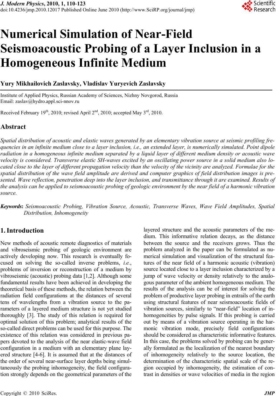J. Modern Physics, 2010, 1, 110-123
doi:10.4236/jmp.2010.12017 Published Online June 2010 (http://www.SciRP.org/journal/jmp)
Numerical Simulation of Near-Field
Seismoacoustic Probing of a Layer Inclusion in a
Homogeneous Infinite Medium
Yury Mikhailovich Zaslavsky, Vladislav Yuryevich Zaslavsky
Institute of Applied Physics, Russian Academy of Sciences, Nizhny Novgorod, Russia
Received February 19th, 2010; revised April 2nd, 2010; accepted May 3rd, 2010.
Abstract
Spatial distributio n of acoustic and elas tic waves generated by an elementary vibration source a t seismic profiling fre-
quencies in an infinite medium close to a layer inclu sion, i.e., an extended layer, is numerically simulated. Point dipole
radiation in a homogeneous infinite medium separated by a liquid layer of different medium density or acoustic wave
velocity is considered. Transverse elastic SH-waves excited by an oscillating power source in a solid medium also lo-
cated close to the layer of different propaga tion velocity than the veloc ity of the vicinity are analyzed. Formulae for the
spatial distribution of the wave field amplitude are derived and computer graphics of field distribution images is pre-
sented. Wave reflection, penetration deep into the layer inclusion, and transmittance through it are examined. Results of
the analysis can be applied to seismoacoustic probing of geologic environment by the near field of a harmonic vibration
source.
Keywords: Seismoacoustic Probing, Vibration Source, Acoustic, Transverse Waves, Wave Field Amplitudes, Spatial
Distribution, Inhomogeneity
1. Introduction
New methods of acoustic remote diagnostics of materials
and vibroseismic probing of geologic environment are
actively developing now. This research is eventually fo-
cused on solving the so-called inverse problems, i.e.,
problems of inversion or reconstruction of a medium by
vibroseismic (acoustic) probing data [1,2]. Although some
fundamental results have been achieved in developing the
theoretical basis of these methods, the relation between the
radiation field configurations at the distances of several
tens of wavelengths from a vibration source to the pa-
rameters of a layered medium structure is not yet studied
thoroughly [3]. The study of this relation is required for
optimal solution of this problem; analytical results of the
so-called direct problem s can be used for this purpose. The
existence of this relation was considered in previous pa-
pers devoted to the analysis of the near elastic-wave field
configuration in a medium with an elementary plane lay-
ered structure [4-6]. It is assumed that at the distances of
the order of several near-surface layer depths being s imul-
taneously the probing inhomogeneity, the field configura-
tion strongly depends on the geometrical parameters of the
layered structure and the acoustic parameters of the me-
dium. This informative relation decays, as the distance
between the source and the receivers grows. Thus the
problem analyzed in the paper can be formulated as nu-
merical simulation and visualization of the structural fea-
tures of the near field of a harmonic acoustic (vibration)
source located close to a layer inclusion characterized by a
jump of wave velocity or density relatively to the analo-
gous parameter of the am bient homogeneous me dium. The
results of the analysis can be of interest for solving the
problem of producti ve lay e r probi ng i n ent rails of t he earth
using structural features of near seismoacoustic fields of
vibration sources, similarly to “near-field” location of in-
homogeneities by pulse signals. If this probing is carried
out by means of a vibration source operating in the har-
monic vibration mode, precisely field configurations
should be considered as characteristic informative features.
In this case, the problems solved by probing can be gener-
ally formulated as the localization of the nearest boundary
of inhomogeneity relatively to the source location, the
determination of the characteristic spatial scale of the re-
gion occupied by inhomogeneity, the estimation of con-
trast in densities or wave velocities of media in the region

Numerical Simulation of Near-Field Seismoacoustic Probing of a Layer Inclusion in a Homogeneous Infinite Medium 111
of inhomogeneity (layer) relatively to internal and external
regions.
Analogous problems ar e set w hen d eter minin g prod uc-
tive layer features in the bottom marine environment,
which are probably present in the characteristics of hy-
droacou stic signals recorded in shelf probing [1,2,7,8].
To extend the application area of the acoustic probing
analysis and generalize it to solid media, we also set
forth the results of numerical simulation of the amplitude
distribution of elastic transverse SH-waves excited by an
oscillating power source located analogously to that in
the previous acoustic case, i.e., at some distance from the
plane parallel layer inclusion having the thickness of one
or several wavelengths. To describe the field of a scalar
medium (liquid or gas), one scalar potential is sufficient,
while the oscillation source is a point oscillating dipole.
To describe elastic SH-waves in a solid medium in the
two-dimensional formulation, we use one component of
the vector potential; a harmonically oscillating power
source uniformly distributed along an infinite line paral-
lel to the layer boundary has the same orientation of the
momentum and radiates transverse SH-waves perpen-
dicular to this line. It is interesting to compare wave pat-
terns of acoustic and elastic-wave fields. First we con-
sider a scalar acoustic field and then results of transverse
elastic wave analysis.
2. Near Acoustic Field of a Point Dipole
Located Close to a Layer Inclusion
in a Homogeneous Infinite Medium
The geometry of the problem is shown in Figure 1.
Three-dimensional infinite space filled with a liquid or
gaseous medium and characterized by the parameters
C
and

, i.e., the density and the acoustic wave veloc-
ity, is separated by a layer infinite in the and
x
y di-
rections and enclosed in the limits hzhH in the
vertical
z
direction; it has the same density

as the
vicinity and differs only by the sound velocity
c(Cс). The source 0
0()() it
F
zrze




is a point
dipole having the power (momentum) 0
F and the os-
cillation frequency

; it is a perturbation in the form of

-functions of the radial
r
and axial
z
coordinates,
oriented along the vertical axis (0
z
is the corresponding
unitary vector), and located at the distance h twice
larger than its thickness
H
relatively to one of the layer
boundaries (this value is taken for definiteness of calcu-
lations). In Figure 1 , the entire space is divided into four
artificially isolated zones (numerated by 1, 2, 3, and 4).
In these four calculation regions due to axial symmetry,
Figure 1. Medium structure and source arrangement for
the “scalar” problem
the acoustic shift field can be described by the scalar
potential

represented for each of them as Fou-
rier-Bessel integrals, i.e., by the following expressions
(the fact or ti e
  is omitted):

(1)
0
0
() iz akeJkr dk 

,0z,


(2)
0
0
() ()
iz iz
bkeb keJkrdk 



,0 zh , (1)


dkkrJekBekB zizi





0
0
)3( )()( 

,
hzhH 

,





0
0
)4( )( dkkrJekd zi

,hHz

,
where

 krJ0 is the zero-order Bessel function, r is the
radial coordinate, k is the radial wave number component,
i.e., the integration variable, 222 kC 

,
222 kс

, and the indefinite coefficients
dBBbba ,,,,,


are further calculated from the
matching conditions of the z-component of the wave
displacements z uand the acoustic pressure
p
at the
boundaries of all the four isolated regions.
The problem is based on the solution of a homogene-
ous acoustic wave equation:
0
1
2
)4,2,1(2
2
)4,2,1( 


 tC


,

Numerical Simulation of Near-Field Seismoacoustic Probing of a Layer Inclusion in a Homogeneous Infinite Medium 112
0
1
2
)3(2
2
)3( 


 tc


; (2)
the source operation is written under the appropriate
boundary condition instead of being written in the
right-hand side of the wave equation:
(2) (1)0
00
0
(0) (0)()
()
2
pz pzFr
FJkrkdk



 
 (3)
The relation between the potential

, the acoustic
pressure
p
, and the z-component of the wave dis-
placement z
u is commonly known:

2
p, zu zz 


(4)
Since the explicit forms of the unknown coefficients
are determined, the expressions for acoustic displace-
ments in all spatial regions are written using standard
expansions:
(1) 02
4
z
iF
u






2
22
0
0
2( )()
11 () ()
iH iH
ih
iH iH
iz
ee
e
ee
eJ krkdk


 







 





 




,


(2) 02
(2 )
022
0
4
2( )()
1() ()
z
iH iH
izihz
iH iH
iF
u
ee
ee ee
Jkr kdk


 
 







 




  




,
(5)

(3) 02
() ()
0
22
0
2
() ()
() ()
z
iHhziHhz ih
iH iH
iF
u
ee
eJ krkdk
ee



 

 



 




(4) 02
()
22
0
2
0
() ()
z
izH
iH iH
iF
u
e
ee
Jkr kdk








 


Specifically, it follows from the latter formula that
field )4(
z
utransmitted through the layer does not depend
on the distance h from the source to the layer bound-
ary closest to it. The first and the last formulae describe
the acoustic wave field traveling for small distances and
also lengths much larger than the wavelength from in-
homogeneity and the source. In this case, the integrals in
Formulae (5) can be asymptotically estimated, while the
wave displacements corresponding to regions 1 and 4
can be giv en by th e expressio ns :
C
R
i
ze
RC
GF
u



2
2
0
)1(
4
)(cos
, (6)
In Formula (7), cH



, Ccc 
,hH


,
and the angle

is measured from the vertical axis z.
The angular characteristics of wave radiation are ob-
tained by Formulae (6) and (7); they show the amplitude
angular dependences for the far backscattered wave
fields )1(
z
u and for the fields traveling forward )4(
z
u.


22 22
22 22
2cos
2222 1sin221sin
22
22 1sin221sin
2cos
()1
1sin cos1sincos1sin
cos1 sincos1 sin
c
i
ic ic
ic ic
c
i
Ge
сс сeссe
ссeссe
e







  
 



 

 


 
 
  
 
 
 
 
 
 
 
 

C
R
i
C
H
i
ze
RcC
iF
u







cos
2
0
)4( )(, (7)



















 



2222 sin1
2
22sin1
2
22
223
sin1cossin1cos
sin1cos
)(cici eссeсс
c,

Numerical Simulation of Near-Field Seismoacoustic Probing of a Layer Inclusion in a Homogeneous Infinite Medium 113
The far field characteristics are displayed in Figures 2(а)
and (b) (in curves 1, 2, and 3,
 5.2,,2 );
these characteristics correspond to waveguide propaga-
tion in the layer, i.e., for 9.0


c. It is seen that in the
far zone, the angular pattern of backscattered waves
changes as the frequency grows, while the directivity of
the field transmitted through the layer remains un-
changed and close to the directivity of the dipole source
oscillating in a homogeneous infinite medium. The cal-
culation results of antiwaveguide propagation for
1.1

c are shown in Figures 3(а) and (b). There is a
considerable difference in the angular d ependences of the
backscattered far field and the field scattered forward.
The characteristic of the field traveling forward is the
occurrence of sharply directed maxima with simultane-
ous presence of the central lobe describing the smooth
dependence. The backscattered field pattern has only
sharply directed maxima analogous to those mentioned
above, as applied to the wave field transmitted through
the layer, which exist there together with smooth lobes.
They, probably, exist due to the so-called nonray waves
[3-6].
The spatial distribu tion of the acoustic field amplitud e
can be also analyzed by means of numerical calculation
of the integrals in Formula (5); in this case, the calcu-
lated distances do not exceed the first tens of wave-
lengths. Since the numerical approach has been em-
ployed, the choice of integral signs eliminating ambigu-
ity in the variable k on two-lobe surfaces and the
choice of the integration methods essential in the ana-
lytical calculations are not discussed.
Now we consider patterns of the spatial amplitude dis-
tribution of the z-component of wave displacements,
which are obtained as a result of numerical simulation
using Formula (5) for the same values of acoustic wave
velocity jump in th e media located inside and outside the
layer, i.e., for the waveguide propagation ccC


0.9 and for the antiwaveguide propagation


c
1.1Cc . Note that the actual pattern of the acoustic
shift field is to be axially symmetrical relatively to the
axis zand can be a set of interleaved axially symmetri-
cal bodies. However in graphical presentation of the am-
plitude field distribution, we use the isometric projection,
in which the field level is represented as relief rising
above the plane z
r
,. The calculated structure of the
acoustic displacement field z
u is shown in Figures
4(а), 4(b), 4(c) and 4(d) for 9.0
Cсc and in
Figures 5(а), 5(b), 5(c) and 5(d) for 1.1
Cсc.
Figure 4(а) displays the field fragment corresponding
to region 1 located behind the source on the opposite side
of the layer region , i.e., for0

z; thus it should be con-
sidered turned in th e opposite direction along the vertical
coordinate z and the corresponding axis in it is denoted -z.
The same scale is used in both axes. The level decrease
is accompanied by the presence of a fan-shaped structure
in the field image over the entire plane, which means the
oscillating depend ence of z uon
r
for constant z or
the oscillating dependence on z for constant
r
. It fol-
lows from the dependence z u on the coordinates that
there is an acoustic radiation maximum directed at a
small angle to the axisz, which is indicated by “eleva-
tion” in the approp riate relief region inclined to this axis.
As distinct from Figure 4(а), in Figures 4(b) and 4(c)
the scale of the axis zis 100 times smaller than the
scale of the axis
r
. The analyzed spatial interval along
the vertical axis amounts to hz 0 in Figure 4(b)
and to hz

hH

in Figure 4(c). In Figure 4(c) for
more detailed consideration of the pattern in the radial

r
direction in the layer region, we used a 10 times
smaller scale. In regions 2 and 3 at larger distances from
the source, the field amplitude sharply decreases both in
radius and vertical z- direction, which is seen in Fig-
ures 4(b) and 4(c). After deep minimum when the face
boundary of the layer is approached, sharp decrease of
the level is changed by the amplitude growth accompa-
nied by its oscillations. Oscillation amplitude decreases
in region 3 are not strong, which indicates that there is
the excitation of several interfering modes in the layer;
each of the resonance frequencies of these modes being
far from the chosen frequency of the source. In region 4
(Figure 4(d)), one can see a comparatively rapid de-
crease of the field level; it is not so sharp as the level
differences in Figures 4(b) and 4(c), if 100-fold scale
difference along zaxis in these figures is taken into
account. The pattern of the near field in region 4 does not
reveal details of the angular co ncentration of the acou stic
field radiated beyond the layer and going to infinity.
Therefore, the calculation data obtained from (7) and
shown in Figure 3(a) supplement the entire field pattern.
At the same time it is evident that even at small d istances,
the field backscattered by the layer has more peculiarities
in its spatial configuration than the field transmitted
through the layer outward has in its amplitude distribu-
tion. If it is assumed that the spatial con figuration can be
the informativeness parameter representing the charac-
teristics of the layer itself, then it is seen from compari-
son that the reflected field contains more information
than the field transmitted on the opposite side. In conclu-
sion of this brief review of the wave pattern it can be
assumed that amplitude oscillations along the radial and
axial coordinates in the near backscattered field is the
consequence of interference of the waves reflected from
the nearest (face) and the second (external relatively to
the source) boundaries. This statement is also applicable to

Numerical Simulation of Near-Field Seismoacoustic Probing of a Layer Inclusion in a Homogeneous Infinite Medium 114
other cases considered below, although wave interference
in the field transmitte d outward is not al ways so strong.
It follows from Figures 5(а) and 5(b), and c that for
ccC
 1.1, the spatial distributions of the wave
amplitudes corresponding to spatial regions 1, 2, and 3
have the forms essentially analogous to those considered
above. There is an apparent difference from the previous
case only in the amplitude d istribution in spatial region 4
corresponding to the field transmitted through the layer
(Figure 5(d)). In the first case, space-angular oscillations
in the transmitted field level were absent; while in con-
sidered case, they are present in the three-dimensional
image of amplitudes. This is indicated by the fan-shaped
angular-periodic structure observed up to some angle to
the vertical axis and similar to the structure shown in
Figure 4(a); its angular periodic repetition is approxi-
mately the same as in region 1. The primary role here is,
probably, played by nonray waves having a rather high
level in the spatial region limited by the sector forming
the angle

 cCarccos



with normal to the bound-
ary [3-6].
Thus in the considered cases, there is some difference
in the entire pattern of the spatial distribu tion of acoustic
fields, which can be used for remote diagnostics of a
probed inhomogeneity. It is evident that spatial ampli-
tude distributions of both the backscattered field and the
field transmitted through the layer should be recorded,
since the near field structure of the acoustic wave transmitted
through inhomogeneity also represents the influence of
Figure 2. Angular field characteristics (а) – (1)
z
u, (b) – (4)
z
u. Curves 1, 2, and 3 – Ω=,,22.5

 , 0.9c
Figure 3. Angular field characteristics: (а) –(1)
z
u, (b) –(4)
z
u. Curves 1, 2, and 3 –Ω=,,22.5

 , 1.1c

Numerical Simulation of Near-Field Seismoacoustic Probing of a Layer Inclusion in a Homogeneous Infinite Medium 115
Figure 4. Fragments of the amplitude distribution pattern of the field
z
u; relief over the coordinate planerz: (а) – Re-
gion 1; (b) – Region 2; (c) – Region 3; (d) – Region 4.

0.9c,

11.1

 hC ,

5

 Hc
the inhomogeneity parameters.
The problems of the backscattered acoustic field of a
dipole harmonic source and of the field transmitted
through a layer inclusion into a homogeneous infinite
medium (when the media differ only in density) are
solved analogously to the stated above. If we consider
the same geometry of the layer-medium structure as in
the case of Figure 1, use the same arrangement of the
source relatively to the boundaries ( h is the distance
between the source and the face boundary of the layer
and
H
is the layer thickness), and assume that the sound
velocity C is equal everywhere, the density of the me-
dium in the v icinity is 1

, while in the la yer is 2

, it is
easy to obtain the following expressions for the acoustic
displacements in the reflected acoustic field )1(
z
uand the
acoustic field )4(
z
utransmi tted t hrough the lay er:
1
2
(1) 2() 00
20
121
12
2cos( )sin( )
1()
42cos( )sin( )
ih ihH iz
z
HiH
iF
ue eeJkrkdk
Hi H


 

 



 



 




 







, (8)

Numerical Simulation of Near-Field Seismoacoustic Probing of a Layer Inclusion in a Homogeneous Infinite Medium 116
Figure 5. Fragments of the amplitude distr ibution pattern of the field
z
u; relief over the coordinate plane rz: (а) – Re-
gion 1; (b) – Region 2; (c) – Region 3, and (d) – Region 4.

c

 ,

9.1

 hC ,

5

 Hc
kdkkrJ
HiH
eiF
uHzi
z











0
0
2
1
1
2
)(
2
1
0
)4( )(
)sin()cos(2
2





. (9)
These formulae are employed to carry out numerical
calculation and analysis of the near acoustic field struc-
ture for different density contrasts in the layer and in the
Vicinity 2121 1, 1

 , enabling one to deter-
mine the influence of variations in the ratio of the densities
in inhomogeneity and in its vicinity. Figures 6 and 7

Numerical Simulation of Near-Field Seismoacoustic Probing of a Layer Inclusion in a Homogeneous Infinite Medium 117
Figure 6. Fragments of the amplitude distribution pattern of the fieldz
u:


10

Ch ,


5CH ,9.0
12



; (а)
– Region 1; (b) – Region 4
Figure 7. Fragments of the amplitude distribution pattern of the field z
u: 10hC



, 5

 C, 21
1.1



; (а)
– Region 1; (b) – Region 4.
deal with fragments of relief above the plane
z
r
,
in
regions 1 and 4, which are calculated by Formulae (8)
and (9) using the same values of the density ratio as in
the velocity ratio calculations, i.e., 210.9,

  21


1
.
1

. These fragments are much similar to those con-
sidered above; the same picture is observed in interme-

Numerical Simulation of Near-Field Seismoacoustic Probing of a Layer Inclusion in a Homogeneous Infinite Medium 118
diate regions 2 and 3, thus neither appropriate fragments
are shown nor are calculation formulas for these regions.
It is seen in Figure 6(а) that if the media differ in density
(9.0
12 


), the distribution of the backscattered
acoustic field is characterized (as in the previous case) by
amplitude decrease and fan –shaped relief but of lower
angular periodicity than that in Figure 4(а). The level of
the field transmitted through the layer (see Figure 6(b))
decreases at larger distances from the external boundary
but angular periodicity of amplitude values is absent. For
a higher density contrast, i.e., for 1.1
12 


(see
Figures 7(а) and 7(b)), the amplitude distribution pat-
terns in reflected waves and waves transmitted through
the layer remain practically invariable, which indicates a
weak influence of the density contrast variation on the
near acoustic field configuration in the layer – vicinity
structure, as distinct from the previously considered ve-
locity jump.
Generally, when comparing differentiation of media in
density and velocity inside and outside the layer, we
come to the conclusion that the sound speed jump in
homogeneity causes a more pronounced variation of the
near field configuration; thus the search system sensitiv-
ity to variation of this parameter is higher than the sensi-
tivity to density contrast variation. This is the main dis-
tinction of these cases, which should be taken into ac-
count in the search for inhomogeneities and can be con-
sidered as one of the diagnostic properties enabling one
to differentiate “inhomogeneities in density” and “inho-
mogeneities in velocity”.
Therefore, the obtained fragments of the near acous-
tic field of a dipole harmonic source operating close to
a layer inclusion yield the entire field pattern in princi-
pally different cases of velocity and density contrasts
inside and outside inhomogeneity. The revealed peculi-
arities provide qualitative information on their applica-
bility as informative attributes in the search for inho-
mogeneity. The distance from the source to the nearest
(face) boundary of the layer, the thickness of the layer,
and hence the sound speed (density) in region 3, i.e., in
the zone occupied by probed inhomogeneity, is deter-
mined by the field configurations in regions 1, 2, and 4.
Thus remote reading of the inhomogeneity parameters
in the harmonic oscillation mode requires “reflection”
and “transmittance” probing. More detailed numerical
simulation of near fields will provide quantitative data
on the relation of inhomogeneity contrast against the
vicinity to the spatial structures of these fields in the
parameters of density and sound speed. Finally, it can
be noted that the illustrations confirm our statements
only qualitatively; the problem of frequency choice
optimization required for practical acoustic probing is
not considered.
3. Transverse SH-Wave Field Generated in
an Infinite Medium by an Extended
Oscillating Power Source Close to a Layer
Inclusion (Two-Dimensional Problem)
The considered vibration source ti eyxzZ



)()(
0
0

is the “force oscillating with the frequency

” (the force
vector is parallel to the unit vector 0
z

and has the am-
plitude 0 Z; the factor ti e
 is omitted as previously) is
uniformly distributed along the axis z due to the
two-dimensional approximation used in the analysis (see
Figure 8). The source is omnidirectional relatively to
radiated SH-waves, i.e., in the plane x, y oriented nor-
mally to the 0 z

direction. Thus besides comparing
acoustic and vibroseismic cases in this analysis, it is pos-
sible to study the influence of the source directivity on
the near field characteristics. As in the previous case, the
layer occupies the spatial region ,



x
h

Hhy


,





z. The vicinity is characterized
by the transverse wave velocity t
C and differs from the
analogous value ct inside the layer; both media have the
same density

.
It is shown in References [4-6] that to describe the wave
displacements z u in the two-dimensional problem, it is
sufficient to introduce one component of the vector poten-
tial x

satisfying the homogeneous wave equation:
0
1
2
)4,2,1(2
2
)4,2,1( 


 tC x
t
x


,
0
1
2
)3(2
2
)3(


 tc x
t
x


. (10)
By analogy with the previous case of a dipole source
in a scalar medium, the entire space is divided into four
especially distinguished regions (see Figure 8); in each
region the value x

is represented as the Fourier ex-
pansion, i.e., by the following expressions:
dkekA ikxyi
xt




)(
)1(

, 0y,

(2) () ()
tt
iyiy ikx
x
B
keCkee dk 



,
hy

0, (11)

(3) () ()
tt
iyiy ikx
xakebkee dk





,

Numerical Simulation of Near-Field Seismoacoustic Probing of a Layer Inclusion in a Homogeneous Infinite Medium 119
Hhyh






dkekD ikxyi
xt
)(
)4(

,


 yHh
where 222 kСtt 

, 222 kctt 

,
tt candC are the shear wave velocities in the vicinity
and inside the layer and k is the integration variable.
The oscillation displacements z uand significant
stresses in the considered waves yz

are expressed
through x

using differential operations:
yu xz  )4..1()4..1( 
, (12)
yuСztyz  )4,2,1(2)4,2,1( 
,yuсztyz)3(2)3(

, (13)
where

is the density of the medium; the source opera-
tion is described by one of the conditions for 0

y
instead of appropriate expressions in the right-hand side
of Equation (10). The boundary condition is:
)()0()0( 0
)1()2( xZyy yzyz
  (14)
The unknown coefficients (), (),(),
A
kBkCk (),ak
(),bk ()Dk are found by matching the indicated shift
components and strains at the boundaries of the four dis-
tinguished regions. Omitting intermediate calculations,
we write down the resultant expressions for the wave
displacements:




























































dk
e
e
e
C
c
e
C
c
H
C
c
i
C
iZ
u
t
ikxyi
hi
Hi
tt
tt
Hi
tt
tt
t
tt
tt
t
z
t
t
tt
2
2
2
2
2
2
2
24
24
2
0
)1(
11
)sin(12
1
4





,


 

























































dk
e
e
C
c
e
C
c
eH
C
c
i
e
C
iZ
u
t
ikx
Hi
tt
tt
Hi
tt
tt
hyi
t
tt
tt
yi
t
z
tt
t
t





2
2
2
2
2
2
)2(
24
24
2
0
)2(
11
)sin(12
4
, (15)






























































dk
e
e
C
c
e
C
c
e
C
c
e
C
c
C
iZ
u
t
ikxhi
Hi
tt
tt
Hi
tt
tt
hHyi
tt
tt
hHyi
tt
tt
t
z
t
tt
tt





2
2
2
2
2
2
)(
2
2
)(
2
2
2
0
)3(
11
11
2,


 






























dk
e
C
c
e
C
c
e
C
ciZ
u
Hi
tt
tt
Hi
tt
tt
t
ikxHyi
t
t
t
z
tt
t




2
2
2
2
2
2
2
)(
4
2
0
)4(
11
It follows from (15) that similarly to the previous case
with an acoustic dipole, the field )4(
z
u does not depend
on the parameterh, i.e., the distance between the source
and the nearest layer boundary, which is the consequence
of the unlimited scale of inhomogeneity along the coor-
dinate
x
and the absence of absorption in the medium.
The obtained expressions are used in the numerical cal-
culation enabling one (by means of computer graphics)
to visualize the spatial distribution of wave amplitudes at
the distances of up to several tens of wavelengths from
the source for the layer thickness of the order of or
smaller than the wavelength and to analyze the peculiari-
ties of this spatial distribution. Specifically, these ex-
pressions are used to make calculations and obtain pat-
terns of the wave displacement field (in the isometric
projection) for the relative distance from the source and
the layer thickness assigned in the dimensionless form:


9

t
Ch ,


5

t
c
H
. As previously, the calcu-
lations are carried out for two velocity jumps
9.0

t
tCc and 1.1

t
tCc . As the integral expres-
sions, each of th e four fragments of the field pattern cor-
responds to its spatial region; the amplitude distribution
is shown as a relief rising above the plane
y
x
,.
Figures 9(a), (b), (c), and (d) should be considered in

Numerical Simulation of Near-Field Seismoacoustic Probing of a Layer Inclusion in a Homogeneous Infinite Medium 120
Figure 8. Mutual arrangement of the source and the layer
scattering of shear SH-waves
the following sequence: Figure 9(а) – region 1, Figure
9(b) – region 2, etc., while for obtaining the entire field
pattern in all the regions all the fragments should be
joined. Since Figure 9(а) should be considered turned in
the opposite direction along the transverse coordinate y,
the correspondin g axis in it is denoted -y. It follows from
the given pattern that in region 1 at larger distances from
the source, besides a decrease of the field )1(
z
u we ob-
serve periodic sequences of maxima occupying fan-
shaped angular sectors, which pass into directional lobes
in the far field. Note that the scale of the longitudinal
coordinate x is the same in all the figures, while the scale
of the transverse coordinate y in Figures 9(b) and 9(c) is
two orders smaller than that in Figures 9(а) and 9(d), i.e.,
the unit length in the transverse direction
y
in Figures
9(b) and 9(c) is 100 times larger than that in Figures 9(а)
and 9(d). Taking into account the scale difference it can
be concluded that at larger distances from the source and
approach to the layer boundary in the second region, the
amplitude of the field)2(
z
udecreases even more abruptly
than that in Figure 9(а). The amplitude of the field pe-
netrating into the layer is maximum in the region oppo-
site to the source, decreases abruptly when escaping
along the coordinate
x
(symmetrically on both sides),
and oscillates along the coordinate
y
. It is seen in Fig-
ure 9(c) that waveguide conditions for excitation and
propagation of several first modes of SH-wave occur
inside the layer. The field )4(
z
uoutside the layer (see
Figure 9(d)) also decreases rapidly and the amplitude
distribution in region 4 differs considerably from the
analogous one in region 1. A similar situation is consid-
ered in the first section for a dipole source in the scalar
acoustic problem.
To gain a better understanding of wave reflections
occurred in near-field probing in the near region of the
source, it is expedient to consider antiwaveguide propa-
gation for an inverse jump of SH-wave velocities inside
the layer and in the vicinity, which equals, for example,
1.1
t
tCc .
Figures 10(a), (b), (c), and (d) exhibit analogous frag-
ments of the spatial field distribution in the same format
and in the same spatial regions as in the figure considered
above. Comparison of the amplitude distributions with the
analogous ones of the previous case (Figure 9) shows that
the spatial dependence can be either the same or slightly
different. The near field in the reflection region (Figure
10(а) – region 1) has practically the same structure as in
the previous case. The configurations of the amplitude
distributions in region 2 (Figures 10(b)) in those cases are
also similar. The field configuration in the layer (Figures
10(c)), i.e., in region 3, differs by the absence of periodic
structure indicating the excitation of SH-wave modes, in
spite of the presence of a crest with undulatory amplitude
modulation also typical of the previous case. In region 4
immediately outside the layer limits (see Figures 10(d)),
an increased-amplitude angular sector forms being similar
to that in the scalar acoustic problem.
The revealed peculiarities differentiating the structures
of the near fields traveling in opposite directions from
the layer in waveguide and antiwaveguide cases demon-
strate the possibility of remote diagnostics of elasticity
jump in the media occupying the internal and external
regions of the layer and enable one to accept them as
informative diagnostic attributes applicable, specifically,
for solving problems of remote diagnostics and medium
structure retrieval. Hence the previously formulated
statement on the necessity of reflected and transmitted
wave recording for diagnostics of inhomogeneity in its
near-field probing, which is similar to reflection and
transmittance location, is valid. Generally, similar results
on peculiarities of wave reflection and transmittance
through a layer several wavelengths thick are typical of
the scalar acoustic problem and the problem with a
source exciting SH-waves in an elastic medium.
4. Conclusions
Numerical simulation of near-field probing of inho-
mogeneity (layer inclusion) in acoustic and seismic me-
dia is carried out, which has confirmed its applicability
with the use of near acoustic and elastic fields of har-
monic sources and recording of waves reflected by in
homogeneity and transmitted through it. The study is
based on the analysis of the visual pattern of the spatial
amplitude distribution in near and far wave fields calcu-
lated by the formulae derived in this paper. The simulta-
neously considered angular characteristics of the far
3
4 H+h
2
1
ct ,

Ct ,

Ct ,

Z0
h
0
C
t ,

y
x
z

Numerical Simulation of Near-Field Seismoacoustic Probing of a Layer Inclusion in a Homogeneous Infinite Medium 121
Figure 9. Fragments of the spatial distribution of wave amplitudes of an oscillating source for 0.9
tt
cC, 11.1
t
hC

 ,
=5

t
ωHc : (а) – Region 1; (b) – Region 2; (c) – Region 3; (d) – Region 4
acoustic field do not contradict the revealed peculiarities
of the near field of elementary oscillation sources oper-
ating close to inhomogeneity. The employed values of
inhomogeneity contrast characterize the relation of den-
sities and sound speeds in the layer and ambient acoustic
medium. To predict the distance from the source to the
layer inclusion and to estimate its thickness, the qualita-
tive character of the dependence
C
hc
H


,
(,
tt
H
chC


) should be studied. Complete investiga-
tions require numerical simulation of a number of definite
values of the mentioned parameters in addition to the
given calculations. At the same time, the near field pecu-
liarities found in this paper (even in a limited volume of
simulation data) are useful for optimal arrangement of
sources and recording receivers in design of experiments
on seismic exploration of productive stratum in massif,
characterized by an abrupt decrease of SH-wave velocity.

Numerical Simulation of Near-Field Seismoacoustic Probing of a Layer Inclusion in a Homogeneous Infinite Medium 122
Figure 10. Fragments of the spatial distribution of the wave field for 1.1
tt
cC

, 9.1


t
hC , =5

t
ωHc : (а) – Region 1;
(b) – Region 2; (c) – Region 3; (d) – Region 4
The structures of the near fields of a vibration source,
which are backscattered or transmitted through inho-
mogeneity, should be considered as a set of informative
basic characteristics indirectly indicating the presence of
a stratum with deposit. Shelf investigations of sea bottom
sediments containing gas condensate layers can be simi-
lar to the search for hydrocarbon accumulation in geo-
logic environment on land territories. In some cases, the
search for inhomogeneities using harmonic oscillation
sources can precede pulse location and determine only
tentative information or boundary contours. In other cas-
es, it is expedient to employ near-field probing using
harmonic sources to increase reliability of pulse echo-
sounding of geological structures or prediction accuracy

Numerical Simulation of Near-Field Seismoacoustic Probing of a Layer Inclusion in a Homogeneous Infinite Medium 123
of their characteristics in remote diagnostics [9].
REFERENCES
[1] A. M. Derzhavin, O. V. Kudryavtsev and A. G. Semenov,
“On Peculiarities of Numerical Simulation of a Vector
Wave Field of a Low-Frequency Acoustic Source in the
Ocean Medium,” Akusticheskii Zhurnal, Vol. 46, No. 4,
2000, pp. 480-489.
[2] L. A. Bespalov, A. M. Derzhavin and O. V. Kudryavtsev,
“On Simulation of a Seismoacoustic Field of a Low-
Frequency Source for Variation in the Structure of Ocean
Bottom Thickness, ” Akusticheskii Zhurnal, Vol. 45, No.1,
1999, pp. 25-37.
[3] L. M. Brekhovskikh, “Waves in Layered Media,” Nauka,
Moscow, 1973, p. 343.
[4] Y. M. Zaslavsky and V. Y. Zaslavsky, “Analysis of a
Vibroacoustic Field in an Extended Layer and a Layer-
Semispace Structure,” Izvestiya Vysshikh Uchebnykh Za-
vedenii, Radiofizika, Vol. 7, No. 2, 2009, pp. 151-163.
[5] Y. M. Zaslavsky and V. Y. Zaslavsky, “Analysis of an
Acoustic Field Excited by a Vibration Source in a Layer
and its Vicinity,” Akusticheskii Zhurnal, Vol. 55, No. 6,
2009, pp. 845-852.
[6] Y. M. Zaslavsky and V. Y. Zaslavsky, “Transverse
Waves Excited by a Variable Power Source in a Layer
and its Vicinity,” NNGU Vestnik, Radiofizika, 2009, No.
5, pp. 61-68.
[7] Y. M. Zaslavsky, B. V. Kerzhakov and V. V. Kulinich,
“Vertical Seismic Profiling on a Sea Shelf,” Akusticheskii
Zhurnal, Vol. 54, No. 3, 2008, pp. 483-490.
[8] Y. M. Zaslavsky, B. V. Kerzhakov and V. V. Kulinich,
“Simulation of Wave Radiation and Phased Antenna Re-
ception on the Ocean Shelf,” Akusticheskii Zhurnal, Vol.
53, No. 2, 2007, pp. 264-273.
[9] J. L. Arroyo, P. Breton, H. Dijkerman, et al. “Superior
Seismic Data from the Borehole,” Oilfield Review, Vol.
15, No. 1, 2003, pp. 1-23.