Journal of Modern Physics
Vol. 2 No. 11 (2011) , Article ID: 8647 , 13 pages DOI:10.4236/jmp.2011.211172
Paraconsistent Annotated Logic in Analysis of Physical Systems: Introducing the Paraquantum Factor of Quantization hψ
1Group of Applied Paraconsistent Logic, Santa Cecília University, Santos, Brazil
2Institute for Advanced Studies of the University of São Paulo, Cidade Universitária, São Paulo, Brazil
E-mail: inacio@unisanta.br
Received August 30, 2011; revised October 8, 2011; accepted October 24, 2011
Keywords: Paraconsistent Logic, Paraquantum Logic, Classical Physic, Relativity Theory, Quantum Mechanics
ABSTRACT
We present in this paper an alternative of modeling physical systems through a non-Classical logic namely the Paraconsistent Logic (PL) whose main feature is the revocation of the principle of non-contradiction. The Paraconsistent Annotated Logic with annotation of two values (PAL2v) is a type of PL and has in its theoretical structure the main feature of dealing with contradictions offering flexibility in drawing conclusions. Several works about applications of PAL2v have shown that such logic is able to provide us with an adequate treatment to uncertainties. Based on the foundations of the PAL2v we presented the ParaQuantum logic (PQL) with the goal of performing analysis of signals from information sources which model physical systems. The formalization of the concepts of the logics PQL, that it is represented in a Lattice, requires the considering of Paraquantum logical states ψ which are propagated through variations of the evidence Degrees µ and λ which come out from measurements performed in Observable Variables in the physical world. When we analyze the lattice of the PQL, we obtain equations which quantify values of physical quantities from where we obtain the effects of propagation of the Paraquantum logical states ψ. In this paper, we introduce the Paraquantum Factor of quantization hψ whose value is associated with a special logical state on the lattice which is identified with the Planck constant h. We conclude through these studies that the Paraquantum Logical Model based on the ParaQuantum logics PQL can link the several fields of the physical sciences by means of quantization of values. It is an innovative approach of formulating natural phenomena.
1. Introduction
Physics, as the science through we can study nature, has in its foundations measurements and mathematical computations which are based on laws of Classical logic concepts [1,2]. In some cases, the limits imposed by the Classic Logic influences in the results of analyses of Physical Systems [3].
It is possible through the non-Classic logics to develop physical models which are capable of treating uncertainty conditions in fields which deal with extreme values such as quantum mechanics and relativity theory [3,4].
We present in this paper an alternative of modeling physical systems through a non-Classical logic namely the Paraconsistent Logic (PL) whose main feature is the revocation of the classic logic principle of non-contradiction. In other words, in its foundation this Paraconsistent logic is capable of dealing with contradictory signals [4-7].
Important research has been made in the projects of expert systems based on algorithms originated from a non-Classical logic, namely Paraconsistent Annotated logic with annotation of two values (PAL2v) [8]. The applications of PAL2v have been successful in the development of expert systems that have to make decisions based on uncertain or contradictory information [9,10]. In these applications of the PAL2v there was the need of some restrictions on the algorithms because in certain conditions the model presented values which were generated through jumps or unexpected variations. Results of more recent research showed us that the restrictions were imposed on the PAL2v because it has features in its basic structure such that the results obtained can be identified with phenomena watched in the study of quantum mechanics [11-14]. In this paper these special features of the PAL2v are studied in the form of variations of values from the concepts of the Paraquantum logic PQL where these phenomena are called Paraquantum Leaps.
We begin the next section introducing Paraconsistent logic (PL) and their main fundamental ideas necessary to the comprehension of this paper. For more information on Paraconsistent logics, we refer the reader to [3,4,6,8].
1.1. The Non-Classical Paraconsistent Logics
Among the several non-Classical logics we have Paraconsistent logics whose main feature is the revocation of the principle of non-contradiction [3,8]. The initial systems of the Paraconsistent logics containing all logical levels such as propositional and predicate calculi as well as logics of superior order are due to N.C.A. da Costa [2,4,5]. There are also Paraconsistent systems for set theory which are strictly stronger that the classic theory so that the classic theory can be considered as a case of the Paraconsistent systems [6].
1.2. Paraconsistent Annotated Logic
The Paraconsistent Annotated logic (PAL) belongs to a family of Paraconsistent logics and can be represented through a lattice of four vertices. These four vertices represent extreme logical states referring to the proposition that will be being analyzed [1,4,6,8].
1.3. The Paraconsistent Annotated Logic with Annotation of Two Values (PAL2v)
According to [8] we can obtain through the PAL a representation of how the annotations or evidences express the knowledge about a certain proposition P. This is done through a lattice on the real plane with pairs (m, λ) which are the annotations as seen in Figure 1.
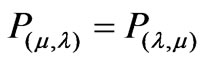
In this representation an operator is fixed: ~:|t| ® |t| where t = {(m, λ)|m, λ Î [0, 1] Ì Â}.
And defined as follows: if P is a basic formula then ~ [(m, λ)] = (λ, m) where m, λ Î [0, 1] Ì Â.
The operator ~ stands for the “meaning” of the logical symbol of negation of the system to be considered.
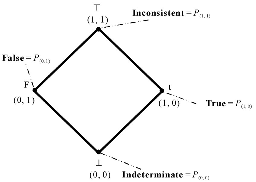
Figure 1. Lattice of four vertexes and representation of the Paraconsistent logical signal: P(m, λ).
We introduce the extreme logical Paraconsistent states which are the four vertices of the lattice with Favorable Degree of evidence μ and Unfavorable Degree of evidence λ. We read them in the following way:
PT = P(1, 1) → The annotation (m, l) = (1, 1) assigns intuitive reading that P is inconsistent.
Pt = P(1, 0) → The annotation (m, l) = (1, 0) assigns intuitive reading that P is true.
PF = P(0, 1) → The annotation (m, l) = (0, 1) assigns intuitive reading that P is false.
P^ = P(0, 0) → The annotation (m, l) = (0, 0) assigns intuitive reading that P is Indeterminate.
In the internal point of the lattice which is equidistant from all four vertices, we have the following interpretation:
PI = P(0.5, 0.5) → The annotation (m, l) = (0.5, 0.5) assigns intuitive reading that P is undefined.
The logical negation of P is defined as:
1.4. The Lattice of the PAL2v
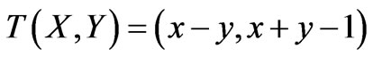
With the values of x and y that vary between 0 and 1 and being considered in an Unitary Square on the Cartesian Plane (USCP) we can get linear transformations for a Lattice k of analogous values to the associated Lattice τ of the PAL2v [8]. We obtain the following final transformation:
 (1)
(1)
Therefore, through the transformation (1) we can convert points of the USCP which represent annotations of τ into points of k which also represent annotations of τ (see [4-6,8]). According to the language of the PAL2v we have:
x = m is the Favorable evidence Degree y = λ is the Unfavorable evidence Degree.
The first coordinate of the transformation (1) is called Certainty Degree DC. So, the Certainty Degree is obtained by:
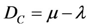 (2)
(2)
The second coordinate of the transformation (1) is called Contradiction Degree Dct. So, the Contradiction Degree is obtained by:
 (3)
(3)
The second coordinate is a real number in the closed interval [–1, +1]. The y-axis is called “axis of the contradiction degrees”.
1.5. The Paraconsistent States Logic (τ
Since the linear transformation T(x, y) shown in (1) is expressed with evidence Degrees μ and λ, from (2), (3) and (1) we can represent a Paraconsistent logical state eτ into Lattice τ of the PAL2v [8], such that:
 (4)
(4)
or
 (5)
(5)
where:
eτ is the Paraconsistent logical state.
DC is the Certainty Degree obtained from the evidence Degrees μ and λ.
Dct is the Contradiction Degree obtained from the evidence Degrees μ and λ.
Since the Paraconsistent logical state eτ can be anywhere in the lattice τ, the real Certainty Degree DCR can be obtained as follows:
For  we compute:
 (6)
(6)
For  we compute:
 (7)
(7)
where:  and
and 
For DC = 0 we consider the undefined Paraconsistent logical state with: DCR =0.
Through (8) we compute the resulting evidence Degree which expresses the intensity of the Paraconsistent logical state ετ.
 (8)
(8)
where:
 is the resulting evidence Degree in function of μ and λ.
 is the real Certainty Degree calculated by (6) or (7).
2. The Paraquantum Logic—PQL
Based on the previous considerations about the PAL2v [8], we present the foundations of the Paraquantum Logics PQL as follows.
2.1. The Paraquantum Function ψ(PQ) and the Paraquantum Logical State ψ
A Paraquantum logical state ψ is created on the lattice of the PQL as the tuple formed by the certainty degree DC and the contradiction degree Dct. Both values depend on the measurements perfomed on the Observable Variables in the physical environment which are represented by μ and λ. We can express (2) and (3) in terms of μ and λ obtaining:
 (9)
(9)
 (10)
(10)
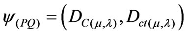
A Paraquantum function y(Py) is defined as the Paraquantum logical state y:
 (11)
(11)
2.2. The Paraquantum Lattice of States of the PQL For each measurement performed in the physical world of μ and λ, we obtain a unique duple  which represents a unique Paraquantum logical state ψ which is a point of the lattice of the PQL.
On the vertical axis of contradictory degrees, the two extreme real Paraquantum logical states are:
1) The contradictory extreme Paraquantum logical state which represents Inconsistency T:
2) The contradictory extreme Paraquantum logical state which represents Undetermination ^:

On the horizontal axis of certainty degrees, the two extreme real Paraquantum logical states are:
1) The real extreme Paraquantum logical state which represents Veracity t:
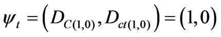
2) The real extreme Paraquantum logical state which represents Falsity F:
2.3. The Vector of State P(ψ)
A Vector of State P(ψ) will have origin in one of the two vertexes that compose the horizontal axis of the certainty degrees and its extremity will be in the point formed for the pair indicated by the Paraquantum function:
 .
.
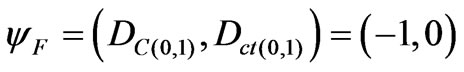
If the Certainty Degree is negative (DC < 0), then the Vector of State P(ψ) will be on the lattice vertex which is the extreme Paraquantum logical state False: ψF = (–1, 0).
If the Certainty Degree is positive (DC > 0), then the Vector of State P(ψ) will be on the lattice vertex which is the extreme Paraquantum logical state True: ψt = (1, 0).
.If the certainty degree is nil (DC = 0), then there is an undefined Paraquantum logical state ψI = (0.5, 0.5).
The Vector of State P(ψ) will always be the vector addition of its two component vectors:
 Vector with same direction as the axis of the certainty degrees (horizontal) whose module is the complement of the intensity of the certainty degree:
 Vector with same direction as the axis of the contradiction degrees (vertical) whose module is the contradiction degree:
Given a current Paraquantum logical state ψcur defined by the duple  then according to (5) we compute the module of a Vector of State P(ψ) as follows:
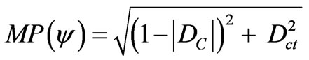 (12)
(12)
where:
DC = Certainty Degree computed by (9)
Dct = Contradiction Degree computed by (10).
Figure 2 shows a point (DC, Dct) where DC = ƒ(μ, λ) and Dct = ƒ(μ, λ) which represents a Paraquantum logical state ψ on the lattice of states of the PQL.
Using (12) which is for computing the module of a
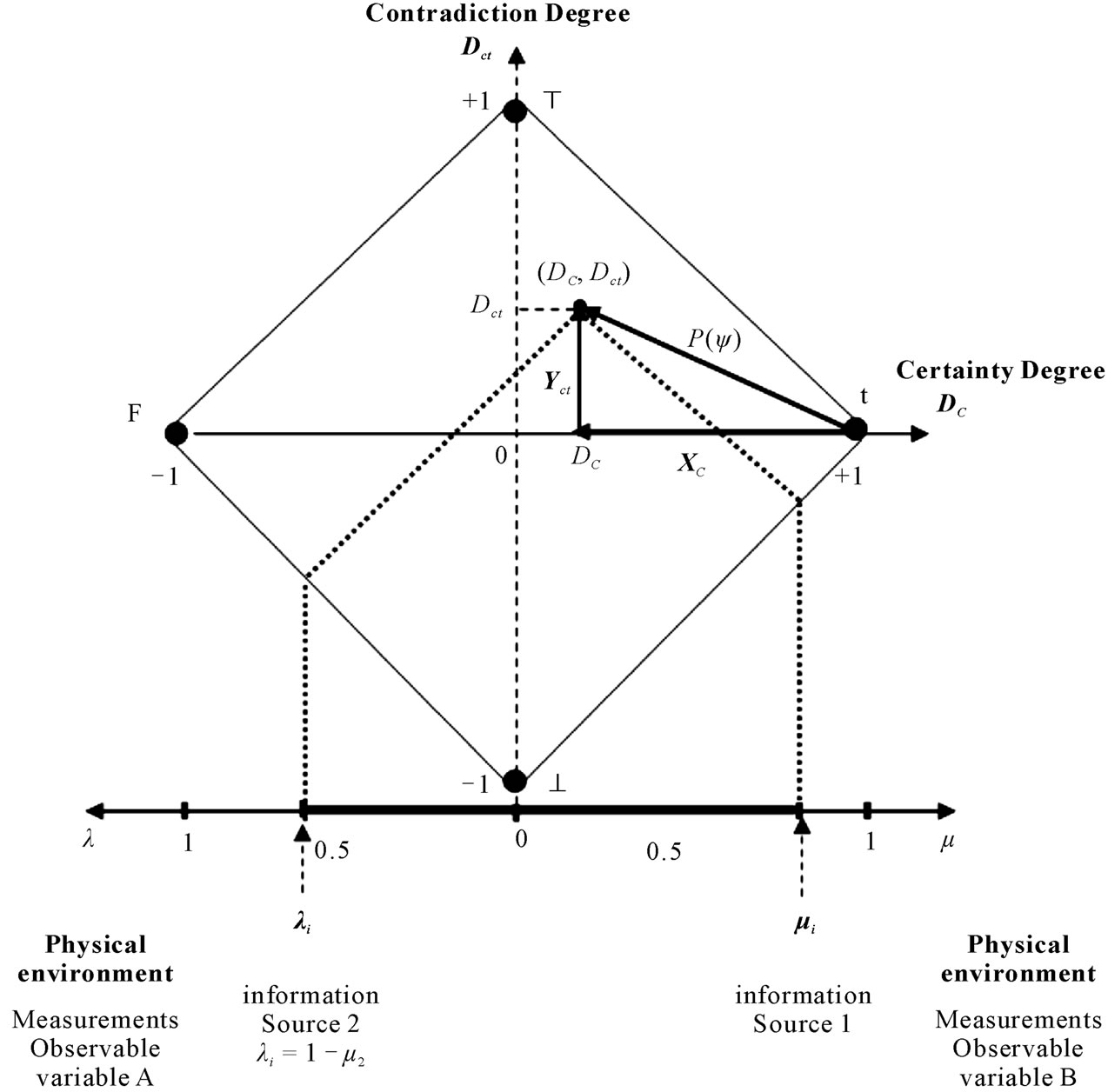
Figure 2. Vector of State P(ψ) representing a Paraquantum logical state ψ on the Paraquantum lattice of states on the point (DC, Dct), therefore DC > 0.
Vector of State P(ψ), we have:
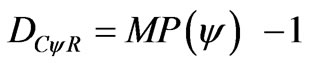
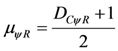
1) For DC > 0 the real Certainty Degree is computed by:
 (13)
(13)
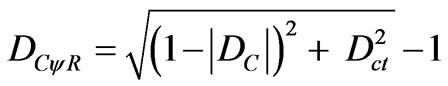
Therefore:
 (14)
(14)
where:
DCψR = real Certainty Degree.
DC = Certainty Degree computed by (9).
Dct = Contradiction Degree computed by (10).
2) For DC < 0, the real Certainty Degree is computed by:
 (15)
(15)
Therefore:
 (16)
(16)
where:
DCψR = real Certainty Degree.
DC = Certainty Degree computed by (9).
Dct = Contradiction Degree computed by (10).
3) For DC = 0, then the real Certainty Degree is nil:

The intensity of the real Paraquantum logical state is computed by:
 (17)
(17)
The inclination angle ay of the Vector of State which is the angle formed by the Vector of State P(y) and the x-axis of the certainty degrees is computed by:
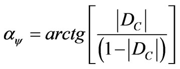 (18)
(18)
The degree of intensity of the contradictory Paraquantum logical state ψctrψ is computed by:
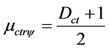 (19)
(19)
where:
μctrψ = intensity degree of the contradictory Paraquantum logical state.
Dct = Contradiction Degree computed by (10).
When the module of the Vector of State MP(ψ) = 1, this vector will represent the maximal fundamental superposed Paraquantum logical states ψsupfmax which has real certainty degrees zero. The maximum Contradiction Degree for this condition is when the Vector of State P(ψ) forms an angle of 45˚ with the horizontal axis of certainty degrees. Therefore, given that the inclination angle of the Vector of State is α = 45˚ then the maximum Contradiction Degree for this condition is computed by:

We observer that this same condition is found when the Vector of State has inclination angle α = –45˚, or still, with origin in the extreme Vertex representative of the extreme False Paraquantum logical state. In that extreme contradictory situation the module of the Vector of State MP(ψ) will have his maximum value of:
 .
.
The unbalanced contradictory Paraquantum logical state ψctru is the one located on the lattice of states of the PQL where there is a condition of opposite signs between the Certainty Degree (DC) and the real Certainty Degree (DCψR).
2.4. Paraquantum Leap and Uncertainty Paraquantum Region
There may be variations in the measurements performed on the observable variables in the physical environment which can dynamically change the values of the evidence Degrees in such a way that the module of the Vector of State MP(ψ) tends to increase. In this situation, as soon as the increase of the module of the Vector of State MP(ψ) becomes greater than 1, the real Certainty Degree DCψR will become greater than 0, that is, the undefined value. This makes DCψR to have the opposite sign of the Certainty Degree DC. In this way, values of real Certainty Degree DCψR will come up and change the logical state of the opposed vertices, even if the Paraquantum logical states defined by the Vector of State P(ψ) are located in the region of the vertex which represents its original logical state. Under this condition a sudden Leap happens in the values of intensity degree of the real Paraquantum logical state μψR computed in (17). This phenomenon where the resultant values are modified abruptly we call Paraquantum Leap.
In the Paraquantum lattice of states of the PQL there is a region where the unbalanced contradictory Paraquantum logical states ψctrd come up. The region of uncertainty on the lattice of states of the PQL is defined by the location of the unbalanced contradictory Paraquantum logical states ψctrd. Therefore, the analysis in this region is as following:
DC > 0 and DCψR < 0 or DC < 0 and DCψR > 0 These are the conditions which define the unbalanced contradictory Paraquantum logical states ψctrd characterized by the Vector of State P(ψ) with module greater than 1.
Since the Favorable evidence Degree μ and the Unfavorable evidence Degree λ in the Paraquantum analysis are originated from the Observable Variables in the physical world, the region of Paraquantum uncertainty is well defined by the increase of decrease of the module of the Vector of State P(ψ) which is related to these values.
3. The Paraquantum Logical State of Quantization yhy
The propagation of the superposed Paraquantum logical states ysup through the lattice of the PQL happens due to the continuous measurements performed on the Observable Variables in the physical world.
Since the Paraquantum analysis deals with Favorable and Unfavorable evidence Degrees m and l of the measurements performed on the physical world, these variations affect the behavior and propagation of the superposed Paraquantum logical states ysup on the lattice of the PQL.
In the propagation of the superposed Paraquantum logical states ysup an equilibrium point exist that is situated on the vertical axis of the degrees of contradiction of the lattice of PQL. The Paraquantum state of quantization yhy is defined as the equilibrium state in the propagation through the uncertainty region of the PQL.
The Paraquantum logical state of quantization yhy which is located in the equilibrium points of the lattice can be obtained through trigonometric analysis. First, we consider the lattice of the PQL as two isosceles triangles with base 2 and height 1.
We observe that from Figure 3, the vertices of these two isosceles triangles are the extreme logical states. On

Figure 3. Correlation of values between the physical world and the Paraquantum universe represented by the lattice of the Paraquantum logics PQL.
the isosceles triangle FTt whose vertices are the extreme Paraquantum logical states false, inconsistent and true, we draw the internal angle bisectors and we find the point I1 (Incenter point) which is the center of the incircle. The point I1 is equidistant from the sides of the isosceles triangle FTt.
The distance from the base, formed by the horizontal axis with the extreme Paraquantum logical states false and true, to I1 is:

This same analysis can be made for other isosceles triangle F^t getting itself thus the correlation of values of balance between the physical world and the lattice of the PQL. Figure 3 shows to this condition of correlation. The lines drawn inside the lattice have inclination of angle α = 45˚ with respect to the horizontal axis. Also, several distances are specified.
Since the normalized values of the Favorable and Unfavorable evidence Degrees m and l are representations of variations occurred in measurements performed on Observable Variables in the physical environment, then the corresponding distances are reflected in the distances of the lattice of the PQL.
The Paraquantum logical states into limits of the Region of Uncertainty of the PQL are those in which the hatched lines with inclination of α = 45˚.
We observe that with respect to the point of Indefinition which is equidistant from the vertices of the PQL, therefore around the Paraquantum logical state of pure Indefinition yIP, the variation of values inside the limits can be expressed by:
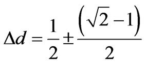 (20)
(20)
These logical states establish connection the incircle point, therefore, in the point where the logical Paraquantum state of quantization yhy is situated.
The Paraquantum logical states into limits of the Region of Uncertainty are identified with Factors of maximum limitation of transition. These factors are:
1) The factor of Paraquantum limitation False/inconsistent—hQyFT.


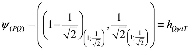
2) The factor of Paraquantum limitation True/inconsistent—hQytT.

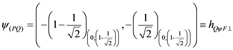
3) The factor of Paraquantum limitation False/undetermined—hQyF^.
4) The factor of Paraquantum limitation True/undetermined—hQyt^.


All the Superposed Paraquantum logical states ysup to these and that they will have variation of the inclination angle until null degree delimit the Region of Uncertainty of the Lattice of PQL.
3.1. The Paraquantum Factor of Quantization hψ
When the superposed Paraquantum logical state ysup propagates on the lattice of the PQL a value of quantization for each equilibrium point is established. This point is the value of the contradiction degree of the Paraquantum logical state of quantization yhy such that:
 (21)
(21)
where:
hy is the Paraquantum Factor of quantization.
The factor hy quantifies the levels of energy through the equilibrium points where the Paraquantum logical state of quantization yhy, defined by the limits of propagation throughout the uncertainty of the PQL, is located.
Figure 4 shows the interconnections between the factors and its characteristics, in which they delimit the Region of Uncertainty in the Lattice of PQL.
In a process of propagation of Paraquantum logical state y, we have that in the instant that the superposed Paraquantum logical state ysup reaches the representative points of the limiting factors of the uncertainty region of the PQL, the Certainty Degree (DC) remains zero but the real Certainty Degree (DCyR) will be increased or decreased from zero and this difference corresponds to the effect of the Paraquantum Leap. So, on the point where
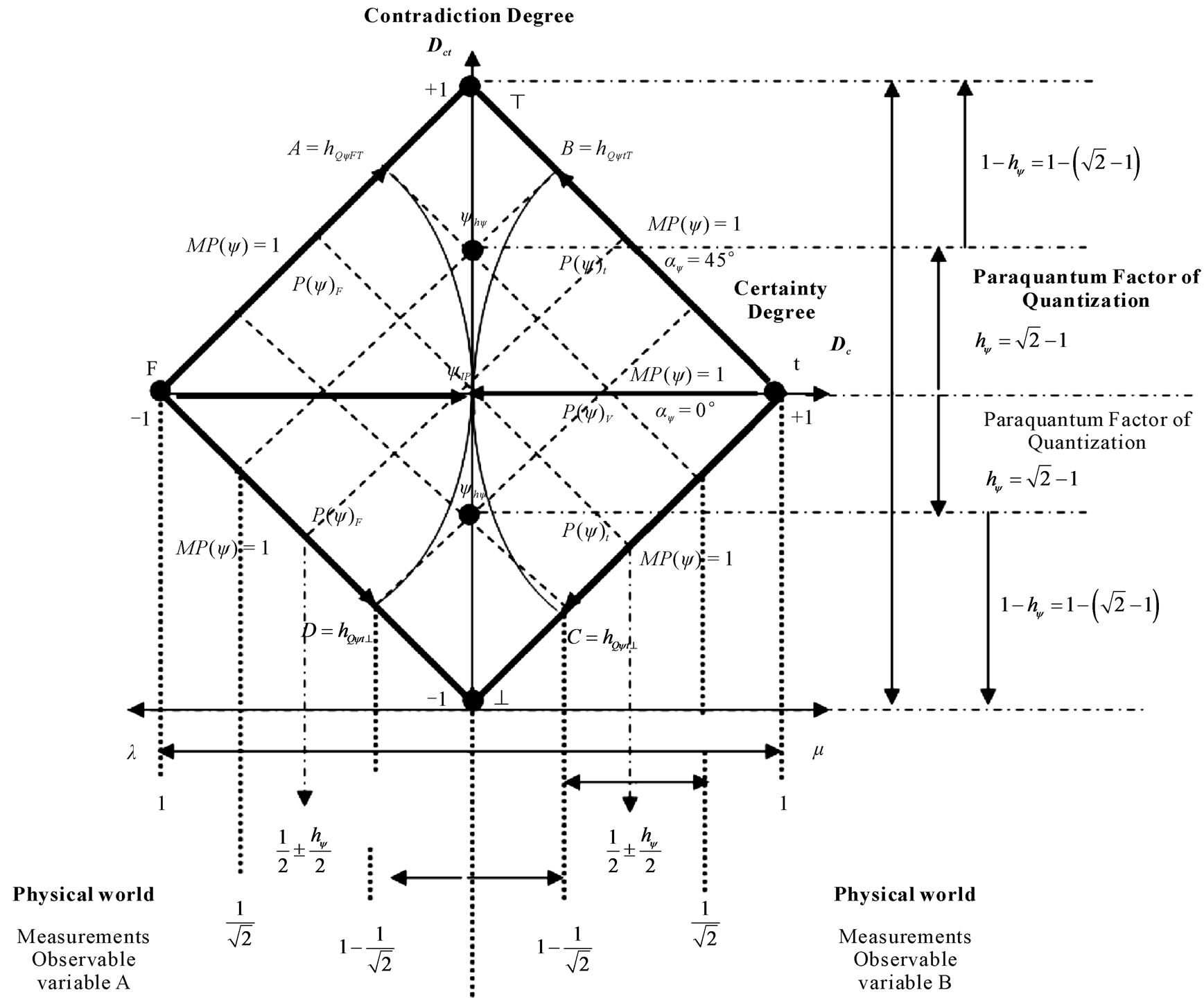
Figure 4. The Paraquantum Factor of quantization hy related to the evidence Degrees obtained in the measurements of the Observable Variables in the physical world.
the logical state of Paraquantum quantization yhy is located, we observe that in the instant of the arrival of the superposed logical states, the Certainty Degree (DC) will be zero but the real Certainty Degree (DCyR) will be increased corresponding to the Paraquantum Leap. In the same way, in the beginning of the propagation, therefore, at the instant that the superposed Paraquantum logical state ysup leaves the point where the logical state of Paraquantum quantization yhy is located, the Certainty Degree (DC) will be zero but the real Certainty Degree (DCyR) will be decreased according to the Paraquantum Leap [6].
At the instant that the superposed Paraquantum logical states ysup visit the Paraquantum logical state of quantization yhy, the real Certainty Degree will have variations of the form:
 (22)
(22)
3.2. The Value of the Paraquantum Leap of Quantization
In a process of propagation of Paraquantum logical state y, we have that in the instant that the superposed Paraquantum logical state ysup reaches the representative points of the limiting factors of the uncertainty region of the PQL, the Certainty Degree DC remains zero, but the real Certainty Degree DCyR will be increased or decreased from zero and this difference corresponds to the effect of the Paraquantum Leap. So, on the point where the logical state of Paraquantum quantization yhy is located, we observe that in the instant of the arrival of the superposed logical states, the Certainty Degree DC will be zero but the real Certainty Degree DCyR will be increased corresponding to the Paraquantum Leap. In the same way, in the beginning of the propagation, therefore, at the instant that the superposed Paraquantum logical state ysup leaves the point where the logical state of Paraquantum quantization yhy is located, the Certainty Degree DC will be zero but the real Certainty Degree DCyR [6] will be decreased according to the Paraquantum Leap. At the instant that the superposed Paraquantum logical states ysup visit the Paraquantum logical state of quantization yhy, the real Certainty Degree will have variations of the form:
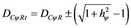 (23)
(23)
Figure 5 shows the details at the instant that the superposed Paraquantum logical states cross the vertical axis of contradiction degrees at the representative point of the Paraquantum logical state of quantization yhy.
During the propagation of the superposed Paraquantum logical states ysup on the lattice of the PQL, a value of quantization for each equilibrium point is established. This is the Contradiction Degree of the Paraquantum logical state of quantization yhy , such that:
 .
.
3.3. The Fundamental Lattice of the PQL We observed that when the Paraquantum logical states ysup visit the Paraquantum logical state of quantization yhy established by the Paraquantum Factor of quantization hy, the Paraquantum Leap happens. In the study of the PQL, when the propagation happens only in this point, the lattice is called fundamental lattice of transition frequency level N = 1. Since that for the fundamental lattice of the PQL, the number of times of application of the Paraquantum Factor of quantization hy is N = 1, then, for a contraction or expansion, the number of times will be greater than 1. Generalizing, we have that the Paraquantum Factor of quantization hy expands or contracts the lattice of the PQL N times such that:
 (24)
(24)
In the physical environment, according to (20) we observe that the maximum evidence degrees, which in the
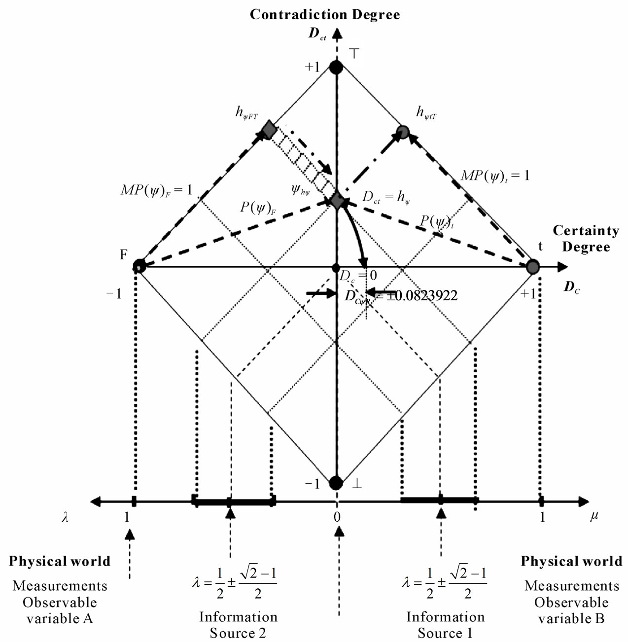
Figure 5. The Paraquantum Factor of quantization hy related to the evidence Degrees obtained in the measurements of the Observable Variables in the physical world.
fundamental lattice of the PQL were 1, become:
 (25)
(25)
In this fashion, the variation around the Paraquantum logical state of pure Indefinition ψIP for the evidence Degrees μ and λ inside the limits of certainty, at each application N of the Paraquantum Factor of quantization hψ:
 (26)
(26)
where:
hψ is the Paraquantum Factor of quantization.
N is the number of times of application of hψ.
In order to completely express it, we have to take into account the factor related to the Paraquantum Leaps which will be added to or subtracted from the Paraquantum Factor of quantization such that:
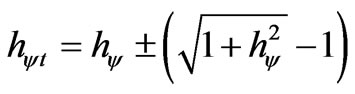 (27)
(27)
Figure 6 shows the effect of the Paraquantum Leap in the quantization of values.
We observe that to hψtn = N it will be added the factor related to the Paraquantum Leap at the arrival of the Paraquantum logical states propagated at the point N or from hψtn = N it will be subtracted the factor related to the Paraquantum Leaps at the arrival of the Paraquantum logical states propagated at the point N.
We can obtain from the fundamental lattice of the PQL the relation between the Paraquantum Factor of quantization hψ and the quantitative value QValor of any physical quantity [15,16] by:
 (28)
(28)
 (29)
(29)
4. The Paraquantum Equation of the Inertial or Irradiant Energy
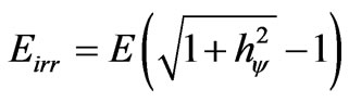
From the Equation (26) we can express the energy of the Paraquantum Leap as the Inertial (or Irradiant) energy
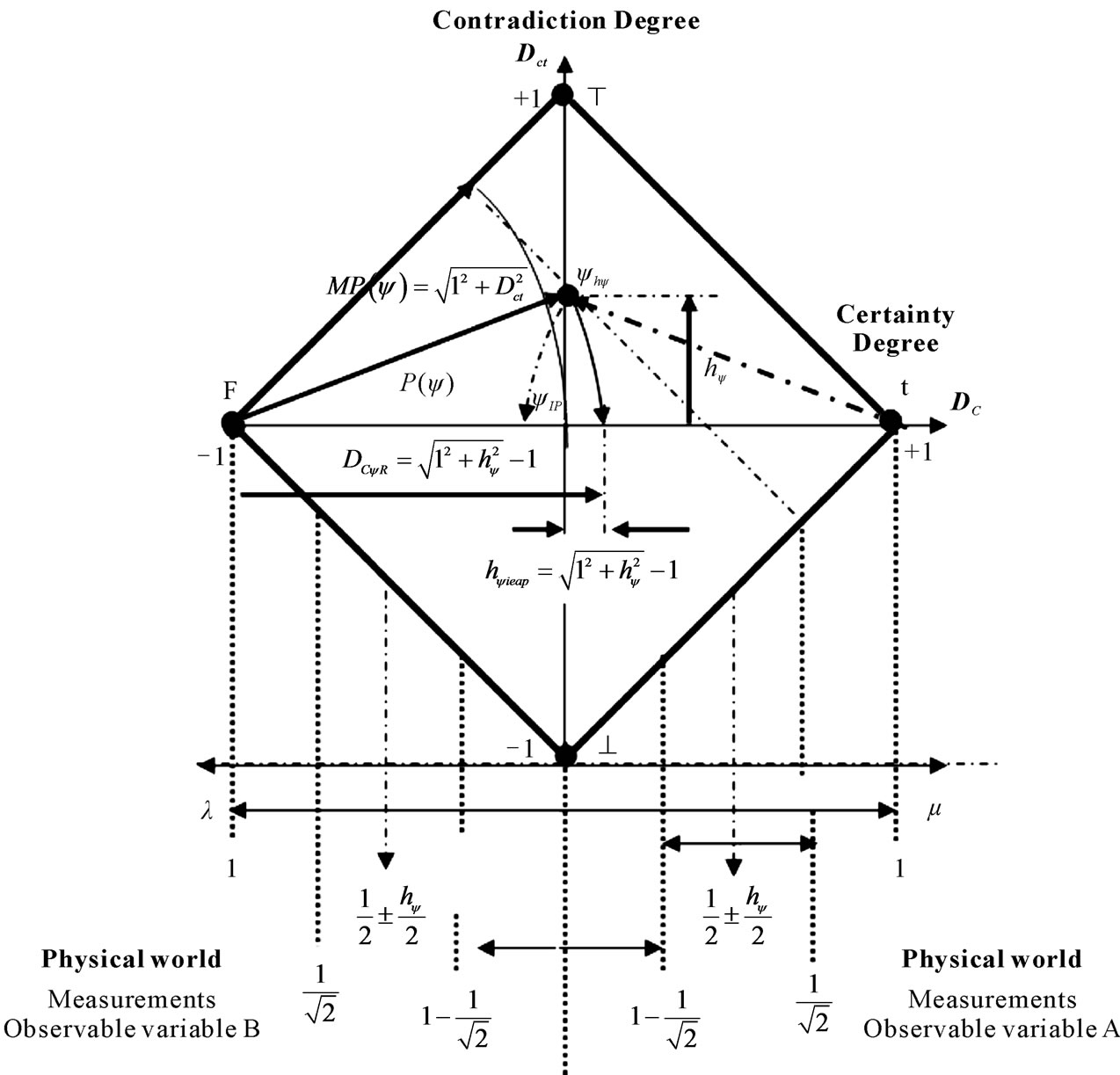
Figure 6. The Paraquantum Factor of quantization on the Paraquantum logical state of quantization yhy due to Paraquantum Leap.
[17,18]. Therefore, this energy is that one that varies when the Paraquantum logical state ψ in its propagation passes for the equilibrium point of the lattice.
 (30)
(30)
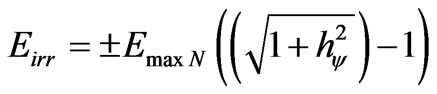
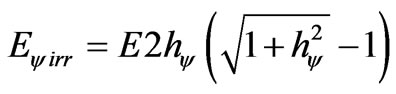
If the maximum energy that is displayed in the horizontal axle of the lattice of Inertial or Irradiant energy is given by , then, in a complete propagation, the Inertial or Irradiant quantized Energy, will be calculated by the application of the Paraquantum Factor of quantization. This condition is express for:
 (31)
(31)
where:
 = quantized Energy of the lattice of Inertial or Irradiant energy.
 = maxima Energy gotten of the lattice of Inertial or Irradiant energy in the fundamental lattice.
 = Paraquantum Factor of quantization.
The multiplication for number 2 must the analysis be in a complete orbit of propagation of the Paraquantum logical state.
4.1. The Paraquantum Planck Constant and Paraquantum Elementary Charge
With Equation (31) we can get in the Lattice of the Inertial or Irradiant Energy, two important constants used in the equations that shape the phenomena of the Physical Systems. Being the Inertial or Irradiant Energy calculated by:
 (32)
(32)
Considering the Paraquantum Inertial or Irradiant Energy (31): .
.
Then, (31) in (32):
 (33)
(33)
Of the Equation (33) it can be extracted the following constants:
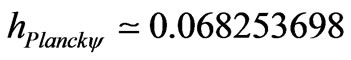
1) The Paraquantum Planck constant  such that:
 (34)
(34)
2) The Paraquantum elementary charge:
 (35)
(35)
As , then from (35) Paraquantum elementary charge is:

The Paraquantum Factor of quantization  and the Paraquantum Planck constant
  are correlation by:
 (36)
(36)
As , then the Paraquantum Planck Constant value is:

The Equation (31) of the Paraquantum Inertial or Irradiant Energy is writing as:
 (37)
(37)
or:
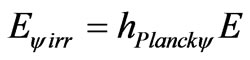 (38)
(38)
Considering the elementary charge |e| used in physical equations of value:

This value can be written as:

Then, the Paraquantum elementary charge of the Equation (35) when inserted in the International System (IS), it can be written as:
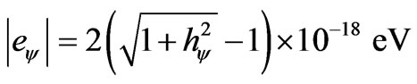
or, when expressed with the value of the Paraquantum Factor of quantization: 
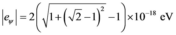
where results in:


In the same way, being the Planck’s constant h [18,19] given in electron-volts x seconds:
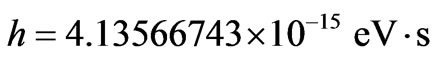
The Paraquantum Planck’s constant  made calculations by the Equation (36), when considered in that same unit it will be inserted in the International System (IS):
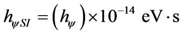
or, when expressed with the value of the Paraquantum Factor of quantization: 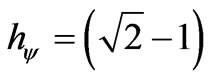
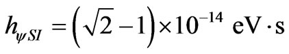
where results in: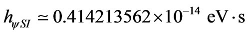 .
.
4.2. The Paraquantum Planck Constant in Reduced Form
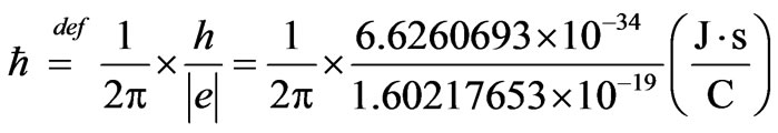
In the calculations of the physical science, mainly the ones that treat in the area of the Quantum Mechanics, they are used in some equations the reduced Planck constant, also known as constant of Dirac.
The reduced Planck constant appears with the symbol , that, by definition, it is made calculations for:

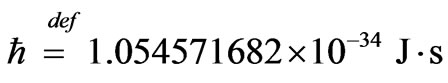
As the module of the elementary charge of the electron is:

Then, the reduced Planck constant in electron-Volt x sec it is made calculations for:

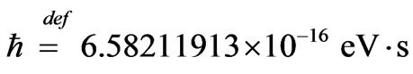
That it can be written as:

This way, being the Paraquantum Planck constant of the Equation (36): 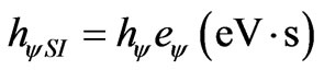
The reduced Planck constant is:
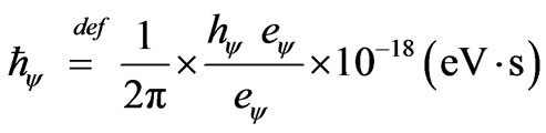
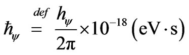
or, when expressed with the value of the Paraquantum Factor of quantization: 
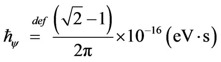
where results in:

5. Conclusions
Based on the concepts of the Paraquantum logics PQL we did in this work a detailed study about the existing correlations between the physical world represented by the values of the evidence Degrees and the Paraquantum world, represented by the lattice of the PQL. The equations and forms of dealing with representative values of physical systems considered on the lattice of the PQL allowed to obtain behavioral characteristics of Paraquantum logical states ψ which produce quantitative results affected by the measurements performed on the Observable Variables in the physical environment. We presented the values which correlate the measurements of the evidence degrees in the physical environment with the quantization factors of the Paraquantum world.
With the results obtained from these considerations, we advanced significantly in the formalization of the model which will allow direct applications of the fundamental ideas of the Paraquantum Logics PQL in analysis of phenomena found in many fields of physics. We saw as if it correlates the Paraquantum Factor of quantization hψ with the values used in the Physics the Planck constant h and the elementary charge e.
The correlation between the extraction of evidence degrees in the physical world, with the Paraquantum Factor of quantization hψ, allows that the Paraquantum logical model to be capable of analyzing physical quantities in a quantitative fashion. For this purpose in the next work we will study as Paraquantum Factor of quantization hψ influences in the physical world, resulting in an important factor of reference that is called of Paraquantum Gamma Factor γPψ.
The model standardizes analysis and interpretations and allows that these applications to be extended to all study areas of physics which are considered incompatible because of existing contradictions in computations.
6. Acknowledgements
The author thanks INESC—Institute of Engineering of Systems and Computers of Porto, Portugal, in particular researcher Prof. Jorge Correia Pereira for the support during this research.
REFERENCES
- S. Jas’kowski, “Propositional Calculus for Contradictory Deductive Systems,” Studia Logica, Vol. 24, 1969, pp. 143-157. doi:10.1007/BF02134311
- N. C. A. Da Costa, “On the Theory of Inconsistent Formal Systems,” Notre Dame Journal of Formal Logic, Vol. 15, No. 4, 1974, pp. 497-510. doi:10.1305/ndjfl/1093891487
- N. C. A. Da Costa and D. Marconi, “An Overview of Paraconsistent Logic in the 80’s,” The Journal of NonClassical Logic, Vol. 6, 1989, pp. 5-31.
- N. C. A. Da Costa, V. S. Subrahmanian and C. Vago, “The Paraconsistent Logic PT,” Zeitschrift fur Mathematische Logik und Grundlagen der Mathematik, Vol. 37, 1991, pp. 139-148. doi:10.1002/malq.19910370903
- R. Anand and V. S. Subrahmanian, “A Logic Programming System Based on a Six-Valued Logic,” AAAI/Xerox Second International Symposium on Knowledge Engineering, Madrid, 1987.
- V. S. Subrahmanian, “On the Semantics of Quantitative Lógic Programs,” Proceedings of 4th IEEE Symposium on Logic Programming, Computer Society Press, Washington DC, 1987.
- D. Krause and O. Bueno, “Scientific Theories, Models, and the Semantic Approach,” Principia, Vol. 11, No. 2, 2007, pp. 187-201.
- J. I. Da Silva Filho, G. Lambert-Torres and J. M. Abe, “Uncertainty Treatment Using Paraconsistent Logic—Introducing Paraconsistent Artificial Neural Networks,” Vol. 211, IOS Press, Amsterdam, 2010, p. 328.
- J. I. Da Silva Filho, A. Rocco, M. C. Mario and L. F. P. Ferrara, “Annotated Paraconsistent Logic Applied to an Expert System Dedicated for Supporting in an Electric Power Transmission Systems Re-Establishment,” IEEE Power Engineering Society—PSC 2006 Power System Conference and Exposition, Atlanta, 29 October-1 November 2006, pp. 2212-2220.
- J. I. Da Silva Filho, A. Rocco, A. S. Onuki, L. F. P. Ferrara and J. M. Camargo, “Electric Power Systems Contingencies Analysis by Paraconsistent Logic Application,” International Conference on Intelligent Systems Applications to Power Systems (ISAP 2007), Toki Messe, 5-8 November 2007, pp. 1-6. doi:10.1109/ISAP.2007.4441603
- C. A. Fuchs and A. Peres, “Quantum Theory Needs no ‘Interpretation’,” Physics Today, Vol. 53, No. 3, March 2000, pp. 70-71.
- M. Ference Jr., H. B. Lemon and R. J. Stephenson, “Analytical Experimental Physics,” University of Chicago Press, Chicago, 1956.
- M. Jammer, “The Philosophy of Quantum Mechanics,” Wiley, New York, 1974.
- J. P. Mckelvey and H. Grotch, “Physics for Science and Engineering,” Harper and Row Publisher, Inc, New York, London, 1978.
- Pl. A. Tipler, “Physics,” Worth Publishers Inc, New York, 1976.
- Pl. A. Tipler and R. A. Llewellyn, “Modern Physics,” 5th Edition, W. H. Freeman and Company, New York, 2007.
- Pl. A. Tipler and G. M. Tosca, “Physics for Scientists,” 6th Edition, W. H. Freeman and Company, New York, 2007.
- H. Reichenbach, “Philosophic Foundations of Quantum Mechanics,” University of California Press, Berkeley, 1944.
- J. A. Wheeler and H. Z. Wojciech (Eds.), “Quantum Theory and Measurement,” Princeton University Press, Princeton, 1983.